Visual Classification: An Interactive Approach to Decision Tree ...

Visual Classification: An Interactive Approach to Decision Tree Construction Mihael Ankerst, Christian Elsen, Martin Ester, Hans-Peter Kriegel Institute for Computer Science, University of Munich Oettingenstr. 67, D-80538 München, Germany { ankerst | elsen | ester | kriegel }@dbs.informatik.uni-muenchen.de

ABSTRACT Satisfying the basic requirements of accuracy and understandability of a classifier, decision tree classifiers have become very popular. Instead of constructing the decision tree by a sophisticated algorithm, we introduce a fully interactive method based on a multidimensional visualization technique and appropriate interaction capabilities. Thus, domain knowledge of an expert can be profitably included in the tree construction phase. Furthermore, after the interactive construction of a decision tree, the user has a much deeper understanding of the data than just knowing the decision tree generated by an arbitrary algorithm. The interactive approach also overcomes the limitation of most decision trees which are fixed to binary splits for numeric attributes and which do not allow to backtrack in the tree construction phase. Our performance evaluation with several well-known datasets demonstrates that even users with no a priori knowledge of the data construct a decision tree with an accuracy similar to the tree generated by state of the art algorithms. Additionally, visual interactive classification significantly reduces the tree size and improves the understandibility of the resulting decision tree. 1. INTRODUCTION Classification is one of the major tasks of data mining. The goal of classification is to assign a new object to a class from a given set of classes based on the attribute values of this object. Different methods [11] have been proposed for the task of classification, for instance decision tree classifiers which have become very popular. Decision tree classifiers are primarily aimed at attributes with a categorical domain, that is a small set of discrete values. Numeric attributes, however, play a dominant role in application domains such as astronomy, earth sciences and molecular biology where the attribute values are obtained by automatic equipment

such as radio telescopes, earth observation satellites and Xray cristallographs. [6] discusses an approach that splits numeric attributes into multiple intervals rather than just two intervals. The well-known algorithms, however, perform a binary split of the form a ≤ v for a numeric attribute a and a real number v. The SPRINT decision tree classifier [3] processes numeric attributes as follows. There are n - 1 possible splits for n distinct values of a. The gini index is calculated at each of these n - 1 points and the attribute value yielding the minimum gini index is chosen as the split point. CLOUDS [4] draws a sample from the set of all attribute values and evaluates the gini index only for this sample thus improving the efficiency. A commercial system for interactive decision tree construction is SPSS CHAID [14] which - in contrast to our approach - does not visualize the training data but only the decision tree. Furthermore, the interaction happens only before the tree construction yielding user defined values for global parameters such as maximum tree depth or minimum support for a node of the decision tree. Visual representation of data as a basis for the humancomputer interface has evolved rapidly in recent years. [8] gives a comprehensive overview over existing visualization techniques for large amounts of multidimensional data. Recently, several techniques of visual data mining have been introduced. [5] presents the technique of Independence Diagrams for visualizing dependencies between two attributes. The brightness of a cell in the two-dimensional grid is set proportional to the density of corresponding data objects. This is one of the few techniques which does not visualize the discovered knowledge but the underlying data. However, the proposed technique is limited to two attributes. [10] presents a decision table classifier and a mechanism to visualize the resulting decision tables. It is argued that the visualization is appropriate for business users not familiar with machine learning concepts. In contrast to well-known decision tree classifiers, our novel interactive approach enables arbitrary split points for numeric attributes, the use of domain knowledge in the tree construction phase and backtracking. In this paper, we introduce a novel interactive decision tree classifier based on a multidimensional visualization of the training data. Our approach allows to integrate the domain knowledge of an expert in the tree construction phase and it overcomes the limitation of binary splits for numeric attributes. The rest of this paper is organized as follows. In

section 2 we introduce our technique for visualizing the training data. The support for interactively constructing a decision tree - which we have implemented in the Perception Based Classification (PBC) system - is discussed in section 3. Section 4 reports the results of an extensive experimental evaluation on several well-known datasets. Section 5 summarizes this paper and outlines several issues for future research.

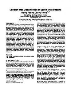
2. VISUALIZING THE TRAINING DATA In our approach, we visualize the training data in order to support interactive decision tree construction. We introduce a novel method for visualizing multi-dimensional data with a class label such that their degree of impurity with respect to class membership can be easily perceived by a user. Our pixel-oriented method maps the classes to colors in an appropriate way. The basic idea of pixel-oriented visualization techniques [8] is to map each attribute value vi of each data object to one colored pixel and to represent the values belonging to different attributes in separate subwindows. The proposed techniques [9] differ in the arrangement of pixels within a subwindow. Circle Segments [2] is a recent pixel-oriented technique which was introduced for a more intuitive visualization of high-dimensional data. The Circle Segments technique maps d-dimensional objects to a circle which is partitioned into d segments representing one attribute each. Figure 1 illustrates the partitioning of the circle as well as the arrangement. Within each segment, the arrangement starts in the middle of the circle and continues to the outer border of the corresponding segment in a line-by-line fashion. These lines upon which the pixels are arranged are orthogonal to the segment halving lines. An extension of this technique has been applied in the context of cluster analysis [1]. To map each attribute 1 attr. 8 attribute value of D to a unique pixel, we follow the idea of the attr. 2 Circle Segments attr. 7 technique, i.e. we represent all values of one attribute in a attr. 3 segment of a circle attr. 6 with the proposed arrangement inside a attr. 5 attr. 4 segment. We do not use, however, the Figure 1. Illustration of the Circle Segoverall distance from ments technique for 8-dimensional data a query to determine objects the pixel position of an attribute value. Instead, we sort each attribute separately and use the induced order for the arrangement in the corresponding circle segment. The color of a pixel is determined by the class label of the object to which the attribute value belongs.

The amount of training data that can be visualized at one time is approximately determined by the product of the number of attributes and the number of data objects. This product minus the number of pixels of a rectangular window not covered by the circle and minus the number of pixels used for the border lines of the segments may not exceed the resolution of the window. For example, 2.000 data objects with 50 attributes can be represented in a 374x374 window and 10.000 objects with 20 attributes fit into a 516x516 window. We have developed a color scale for class labels based on the HSI color model [7], a variation of the HSV model. The HSI model represents each color by a triple (hue, saturation, intensity). In our experiments, we observed the most distinctly perceived colors for the following parameter settings: For col1 we set hue = 2.5 and intensity = saturation = 1.0, for colm we set hue = 0.5 and intensity = saturation = 1.0, and all other colors were obtained by partitioning the hue scale into k – 1 equidistant intervals. A visualization of the resulting color scale is available at http:// www.dbs.informatik.uni-muenchen.de/~ankerst/kdd99/ index.html. Our approach of visualizing the training data also considers attributes having a low number of distinct values. In that case, there are many objects sharing the same attribute value and their relative order is not uniquely defined. Depending on the chosen order, we might create homogeneous (with respect to the class label) areas within the same attribute value. To avoid the creation of artificial homogeneous areas, we use the technique of shuffling: for a set of data objects sharing the same attribute value the required order for the arrangement is determined randomly, i.e. their class labels are distributed randomly.

3. INTERACTIVE CLASSIFICATION Visualization of the corresponding data User selects attribute selects split points Updated Visualization of knowledge User selects one node in tree

User removes one level

User assigns class label to one partition Figure 2. A model for interactive classification

The described visualization of the data is the basis of our

Splitlines

Current State of Decision Tree

Cluster Info about the Selected Attribute Slider

Magnified Splitlines

Figure 3. A Screen Shot of the PBC system

approach of interactive classification. Figure 2 depicts our model for interactive decision tree construction. Initially, the complete training set is visualized in the Data Interaction Window together with an empty decision tree in the Knowledge Interaction Window. The user selects a splitting attribute and an arbitrary number of split points. Then the current decision tree in the Knowledge Interaction Window is expanded. If the user does not want to remove a level of the decision tree, he selects a node of the decision tree. Either he assigns a class label to this node (which yields a leaf node) or he requests the visualization of the training data corresponding to this node. As depicted in figure 3, the latter case leads to a new visualization of every attribute except the ones used for splitting criteria on the same path from the root. Thus the user returns to the start of the interaction loop. The interaction is finished when a class has been assigned to each leaf of the decision tree. Interactive Selection of Split Points The interactive selection of split points consists of two steps: (1) selecting splitlines and (2) selecting a split point on each of the selected splitlines. First, by clicking on any pixel in the chosen segment, the user selects a splitline which is one of the lines (orthogonal to the segment halving line) upon which the pixels are arranged. Then by the system this splitline is replaced with an animated line on which alternatively black and white strips move along. Since the colors black and white are not used for the mapping of the classes, the brushed splitline is well perceptible. In a separate area, the pixels of the selected splitline are redrawn in a magnified fashion which enables the user to set the exact split point. Note that the separation of two different colors is not the only criteria for

determining the exact split point. If not all attribute values on the splitline are distinct, the same attribute values may belong to objects of different classes. In this case, setting a split point between two differently colored pixels would not be reasonable. Hence we provide feedback to the user in both the basis data visualization and the separate splitline area, such that the attribute value of the pixel at the position of the mouse pointer appear in a subwindow. Figure 3 illustrates the visualization support for the selection of a splitline and an exact split point. Splitting strategy Our interactive approach overcomes the limitations of binary splits in attributes with a continuous domain. This additional flexibility rises the question about an appropriate splitting strategy. In our experiments, we observed the best results in terms of accuracy and tree size if the choice of the splitting attribute is based on the strategy described below. The strategy has four options and the first of them which is applicable in the current visualization should be chosen. We will use the term partition for a coherent region of attribute values in the splitting attribute that the user intends to separate by split points. 1) Best Pure Partitions (BPP). First choose the segment with the largest pure partitions. A partition is called pure if the user decides to label this partition with the most frequent class. This decision leads to leaf nodes in the decision tree, thus reducing the size of data which is not classified. 2) Largest Cluster Partitioning (LCP). If no pure partition is perceptible, the segment with the largest cluster clearly dominant in one color should be chosen. In contrast to a pure partition, such a cluster will not be labeled by the most frequent class.

3) Best Complete Partitioning (BCP). If a choice upon BPP or LCP fails, the segment should be chosen that contains the most pixels that can be divided into partitions where each has one clearly dominant color. 4) Different Distribution Partitioning (DDP). If none of the above options applies, choose the segment where different distributions can be best separated through partitioning. After an attribute is chosen the split points have to be set. If the choice follows BPP or LCP, additional split points in the remaining partition should be set if it leads to a separation of clusters or of different distributions. Thus, more inherent information of the splitting attribute is used for deriving the decision tree. Note that the splitting attribute will not reappear in lower nodes of the same path.

4. EXPERIMENTAL EVALUATION In comparison to algorithmic decision tree classifiers, the process of interactive classification reveals additional insights into the data. To illustrate this advantage, in this section we discuss an example of two consecutive steps in the tree construction phase. Furthermore, we compare our classifier with popular algorithmic classifiers in terms of accuracy and tree size...

Figure 4(a) depicts the visualization of the Shuttle data after the selection of the first two splitting attributes. Attributes 1 and 9 are obvious candidates for splitting. According to ’Best Pure Partitions’, attribute 9 should be chosen because in contrast to the larger cluster in the segment of attribute 1, the split leads to a pure partition. Note that the nonhomogeneity of the cluster in attribute 1 can only be perceived in the color representation. The pure partition can be assigned to the class of its only color. The visualization of the remaining partition has to be examined in a further step. This is shown in figure 4(b) representing the data objects visualized in figure 4(a) except for all objects belonging to the pure partition in attribute 9. Attribute 9 is not visualized any more because it was already used as a splitting attribute on this path of the decision tree. One effect of our visual approach becomes very clear in this example the removal of some training objects from the segment of the splitting attribute may yield the removal of objects from another segment which make a partition of this segment impure. For example, the cluster in attrribute 1 (figure 4(a)) becomes a pure partition after the split (figure 4(b)). We used the accuracy and the tree size (total number of nodes) as quantitative measures to compare PBC with wellknown algorithmic approaches. We used the tree size besides accuracy since small trees are easier to understand and we consider understandability of the discovered knowledge to be a major goal. For the comparison, we used three datasets from the Statlog database [12] for which the accuracy and the tree size of many algorithms is known [4]. The Satimage, Segment and Shuttle datasets were chosen because all of their attributes are numeric. We performed the experiments as suggested in the dataset descriptions. As comparison partners we chose the popular decision tree classifiers CART and C4 from the IND package [13] as well as the recently proposed SPRINT [3] and CLOUDS [4] classifiers. The results of CLOUDS were produced with the SSE/DM method. Accuracy

CART

C4

SPRINT CLOUDS

PBC

Satimage

85.3

85.2

86.3

85.9

83.5

Segment

94.9

95.9

94.6

94.7

94.8

Shuttle

99.9

99.9

99.9

99.9

99.9

Tree size

CART

C4

Satimage

90

563

159

135

60

Segment

52

102

18.6

55.2

39.5

Shuttle

27

57

29

41

14.6

(a) Cluster in attribute 1 (b)

Pure partition in attribute 9

Pure partition in attribute 1 Figure 4. Visualization of the Shuttle data before (a) and after a split (b)

SPRINT CLOUDS

PBC

Table1,Table 2: Accuracy and Tree size of PBC and algorithmic approaches

Table 1 depicts the accuracy of PBC and the algorithmic approaches, table 2 their tree sizes. Our performance

evaluation demonstrates that the approach of interactive visual classification yields an accuracy similar to the accuracy obtained by well-known algorithms. PBC significantly reduces the tree size and thus obtains decision trees which are much better understandable. To illustrate this advantage, figure 5 shows a decision tree for the Shuttle dataset constructed with the PCB system. Attribute 7 represents the root of the tree with one split point at 6.0. The following two nodes are the left (attribute 7 < 6.0) and right son of this root. The left son of the root is already assigned to a class (Bypass). The Figure 5. A decision tree for the colored square Shuttle dataset besides the class label depicts the color representing the class. We observe that the nodes with the splitting attributes 1 and 2 both have two split points yielding a 3-ary decision tree that cannot be generated by the algorithmic approaches.

5. CONCLUSION In this paper, we introduced a fully interactive method for decision tree construction based on a multidimensional visualization technique and appropriate interaction capabilities. Thus knowledge can be transfered in both directions. On one hand, domain knowledge of an expert can be profitably included in the tree construction phase. On the other hand, after going through the interactive construction of a decision tree, the user has a much deeper understanding of the data than just knowing the decision tree generated by an arbitrary algorithm. Our approach has several additional advantages compared to algorithmic approaches. First, the user may set an arbitrary number of split points which can reduce the tree size in comparison to binary decision trees that are generated by most state of the art algorithms. Furthermore, in contrast to the greedy search performed by algorithmic approaches, the user can backtrack to any node of the tree when a subtree turns out to be suboptimal. We conducted an experimental evaluation on several popular datasets. We found that even users with no a priori knowledge of the training data construct a decision tree that has a similar accuracy and a significantly smaller tree size compared to algorithmic approaches. In our future work, we will improve the scalability with respect to the maximum amount of data that can be processed. Furthermore, we plan to extend our PBC system by features of algorithmic approaches and we want to

explore methods of integrating PBC with a database management system.

6. REFERENCES Ankerst, M., Breunig M, Kriegel H.-P. and Sander J.:”OPTICS: Ordering Points To Identify the Clustering Structure”, in Proc. ACM SIGMOD ‘99, Int. Conf. on Management of Data, Philadelphia, PA, 1999. [2] Ankerst M., Keim D. A. and Kriegel H.-P.: “Circle Segments: A Technique for Visually Exploring Large Multidimensional Data Sets”, Proc. Visualization ’96, Hot Topic Session, San Francisco, CA, 1996. [3] Agrawal R., Mehta M. and Shafer J.C.: “SPRINT: A Scalable Parallel Classifier for Data Mining”, in Proc. VLDB ‘96, 22nd Intl. Conf. on Very Large Databases, Bombay, India, 1996, pp. 544-555. [4] Alsabti K., Ranka S. and Singh V.: “CLOUDS: A Decision Tree Classifier for Large Datasets”, in Proc. KDD ‘98, 4th Intl. Conf. on Knowledge Discovery and Data Mining, New York City, 1998, pp. 2-8. [5] Berchtold S., Jagadish H.V. and Ross K.A.: “Independence Diagrams: A Technique for Visual Data Mining”, in Proc. KDD ‘98, 4th Intl. Conf. on Knowledge Discovery and Data Mining, New York City, 1998, pp. 139-143. [6] Fayyad U.M. and Irani K.: “Multi-interval Discretization of Continuous-Valued Attributes for Classification Learning”, in Proc. IJCAI ‘93, Int. Joint Conf. on Artificial Intelligence, 1993. [7] Keim D.A.: “Visual Support for Query Specification and Data Mining”, PhD Thesis, University of Munich, Germany, 1994. [8] Keim D. A.: ”Visual Database Exploration Techniques”, Proc. Tutorial Int. Conf. on Knowledge Discovery & Data Mining, Newport Beach, CA, 1997.(http://www.informatik.uni-halle.de/~keim/PS/ KDD97.pdf) [9] Keim D. A., Kriegel H.-P. and Ankerst M.: ”Recursive Pattern: A Technique for Visualizing Very Large Amounts of Data”, in Proc. Visualization ‘95, Atlanta, GA, 1995, pp. 279-286. [10] Kohavi R. and Sommerfield D.: “Targeting Business Users with Decision Table Classifiers”, in Proc. KDD ‘98, 4th Intl. Conf. on Knowledge Discovery and Data Mining, New York City, 1998, pp. 249-253. [11] Mitchell T.M.: “Machine Learning”, McGraw Hill, 1997. [12] Michie D., Spiegelhalter D.J. and Taylor C.C.: “Machine Learning, Neural and Statistical Classification”, Ellis Horwood, 1994. [13] NASA Ames Research Center: “Introduction to IND Version 2.1”, 1992. [14] http://www.spss.com/. [1]