MODIS cloud fraction and outperforms support vector machine (SVM) in terms of estimation performance. Index Termsâ Cloud detection, multiple-kernel.
MULTIPLE-KERNEL LEARNING-BASED UNMIXING ALGORITHM FOR ESTIMATION OF CLOUD FRACTIONS WITH MODIS AND CLOUDSAT DATA Yanfeng Gu a,*, Shizhe Wang a, Tao Shi b, Yinghui Lu c, Eugene E. Clothiaux c, Bin Yu d a
Department of Information Engineering, Harbin Institute of Technology, Harbin, 150001, China Department of Statistics, The Ohio State University, Columbus, OH 43210-1247, United States c Department of Meteorology, Pennsylvania State University, University Park, PA 16802, United States d Department of Statistics, University of California, Berkeley, CA 94720-3860, United States b
ABSTRACT Detection of clouds in satellite-generated radiance images, including those from MODIS, is an important first step in many applications of these data. In this paper we apply spectral unmixing to this problem with the aim of estimating subpixel cloud fractions, as opposed to identification only of whether or not a pixel radiance contains cloud contributions. We formulate the spectral unmixing approach in terms of multiple-kernel learning (MKL). To this end we propose a MKL-based unmixing algorithm that drives a multiple-kernel description of cloud, enabling estimation of sub-pixel cloud fractions. This approach is based on supervised learning. We generate training and testing samples by using CloudSat and CALIPSO data to compute cloud fractions within individual MODIS pixels. Results of our study on limited data (1875 training and testing MODIS pixels along with their CloudSat and CALIPSO based sub-pixel cloud fractions) show that the proposed algorithm can effectively estimate sub-pixel MODIS cloud fraction and outperforms support vector machine (SVM) in terms of estimation performance. Index Terms— Cloud detection, multiple-kernel learning (MKL), MODIS, spectral unmixing 1. INTRODUCTION The Moderate Resolution Imaging Spectroradiometer (MODIS) onboard the NASA Terra and Aqua satellites continually collects radiances in 36 spectral channels for both short- and long-term changes in the Earth’s land, ocean and atmosphere systems [1]. Detection of pixel radiances with cloud contributions is an important first step in the application of MODIS data to many Earth science investigations. To facilitate production of MODIS operational cloud products Ackerman et al. [2] developed a well-documented algorithm for this purpose and clearly describe the information content within the MODIS radiances at the 36 different wavelengths. From these 36 radiances they developed 5 sets of features, via transformations/combinations of these 36 radiances for a pixel, that are subsequently used in single-valued thresholds
tests to separate clear form cloudy pixels. One complication of this approach is that a single set of single-valued thresholds may not apply for all times and regions. Shi et al. [3] investigated detection of daytime arctic clouds at the pixel level by using radiances and features derived from Multi-angle Imaging Spectroradiometer (MISR) and MODIS data. The importance of their work was use of combinations of features from MISR and MODIS and development of a scheme that incorporated adaptable thresholds within Fisher’s quadratic discriminate analysis in order to separate clear and cloudy pixels. The Cloud-Aerosol Lidar and Infrared Pathfinder Satellite Observation (CALIPSO) [4] and CloudSat cloud profiling radar (CPR) were launched in 2006. These two instruments provide global cloud profiles from space. Most importantly for our study, their data are collocated with pixels near the center of the MODIS swath. Joint CPR and CALIPSO vertical cloud profiles are available. We use the variable CloudFraction within the data product, which reports, as a function of altitude, the fraction of lidar beams within a radar beam that contains hydrometeors. CloudFraction is recorded per ray and per bin as a 1-byte integer variable representing a percentage from 0% to 100%. Using CloudFraction together with those MODIS pixels with which it is collocated, it is possible to build a model for estimating cloud fractions in MODIS pixels away from the center of the MODIS swath and for which there are no available CloudFraction data. Two complicating factors for this estimation are the within-class variability of the radiances associated with cloudy MODIS pixels and the existence of mass-mixed (i.e., partially cloudy pixels and cloud-free pixels but with different surface types within them) pixels brought about by the spatial resolution of MODIS. In this paper we address the cloud detection problem using spectral unmixing. First, we model MODIS pixel radiances as linear mixtures of cloud and background. We then propose a multiple-kernel learning (MKL)-based unmixing algorithm to drive a multiple-kernel model or the estimation of cloud fractions at a sub-pixel level. In Multiple-kernel Hilbert space (MKHS) we form class boundaries to represent the cloudy and cloud-free pixel and estimate the sub-pixel cloud fractions.
2. METHODOLOGY
2.2. Spectral mixtures of cloud and background Traditional methods for cloud detection attempt to identify a pixel as either being cloudy or cloud free (or clear). This is not satisfying in that pixels are potentially only partly cloudy. Hence it is more realistic to estimate the fraction of cloudiness within each pixel. To this end, we formulate cloud detection as a problem of spectral unmixing. The 36 MODIS radiances associated with each pixel potentially contain combinations of contributions from clouds and the background. Expressing this as a linear mixture, we have s = ps cloud + (1 − p ) s background + n (1) where s is the spectrum (i.e., the 36-element vector containing the 36 radiances per MODIS pixel) to be categorized, s cloud is the contribution to s from clouds, sbackground is the contribution to s of the background, n is noise and p is the pixel cloud fraction that comes from the variable CloudFraction that is matched with the MODIS pixel. In our study, we also use all of features in the five sets developed by Ackerman et al. [2], calling this 15-element vector x. Let y represent the cloud-fraction label derived from CloudFraction and which is associated with vector x for a MODIS pixel. Here, y=+1 means a cloud fraction of 1 (i.e., fraction p=1), y=-1 means only a background contribution (i.e., fraction p= 0). In this way, we can generate a set of N N training samples { xi , yi }i =1 containing only completely cloudy and clear MODIS pixels. The problem to be solved is estimation of the cloud fractions within the other MODIS pixels of the testing and training data set, after which the model can be applied to any MODIS pixel. The fully constrained least squares (FCLS) method that was proposed in [5] can be used to solve the problem represented by Eq. (1), as can be a support vector machine (SVM) [6], which improves performance for nonlinear spectral mixtures. In Fig.1, we present the main idea of an extended SVM algorithm that is proposed for hyperspectral unmixing in [7,
Feature band 2
2.1. Feature selection for detection of cloud In our study we use the five sets of features provided by Ackerman et al. [2]. These features are based on brightness temperatures (BT) and reflectances (ρ) generated from MODIS radiances and include: (1) BT11, BT13.9, BT6.7 for detecting thick high clouds; (2) BT11-BT12, BT8.6-BT11, BT11BT3.9, BT11-BT6.7 for detecting thin clouds; (3) ρ0.87, ρ0.65, ρ0.936, BT3.9-BT3.7 for detecting low thick clouds; (4) ρ1.38 for detecting upper tropospheric thin clouds; and (5) sensitive brightness temperature differences BT11-BT12, BT12-BT4, BT13.7-BT13.9 for detecting cirrus. Compared with MODIS radiances, these five sets of features generated from them reduce the dimensionality of the 36 radiances and weaken within-class variability.
Class Boundaries +1
Cloud
‐1
D1 D2 Mixed pixels
Background
Feature band 1
Fig. 1 pure and mixed pixels’ locations in feature space
8]. The region between the hyperplanes formed by the pixels on the class boundaries (support vectors) is recognized as containing partly cloudy pixels whereas the other two regions are related to pure pixels. In other words, in Hilbert Space, if a pixel is located between the class boundaries, it is identified as a mixed pixel. If a pixel is located in a region whose SVM output is less than -1, it is identified as a pixel with pure background contributions; otherwise, it is identified as a pure pixel with only cloud contributions. The support vectors located on the hyperplanes +1 and -1 are defined as pure pixels for the two classes. Given the labeled data set {( x i , yi ), i = 1, 2,..., N } , where xi ∈ R L is the input training vector of features with L elements (L is the dimension of the feature space) and yi ∈ {+1, −1} , and given a nonlinear mapping φ ( ⋅) , the standard SVM solves N ⎧1 ⎫ 2 ( w ∗ , b∗ ) = arg min ⎨ w + C ∑ ξ i ⎬ w ,ξ i , b 2 i =1 ⎩ ⎭ ⎧⎪ yi [ w ,φ ( x i ) + b] ≥ 1 − ξ i s.t. ⎨ ⎪⎩ξ i ≥ 0, ∀i = 1,", N
(2)
where w is the vector of parameters which support the optimal decision hyperplane w ∗ ,φ (x) + b∗ = 0 and b is a bias, w* and b* represent the optimal solution to the problem of all possible solutions, ξi is a non-negative slack variable necessary for dealing with noisy and nonlinearly separable data, φ ( i ) is an implicitly defined nonlinear mapping and occursin the form of an inner product which will be replaced with a kernel function K (x i , x j ) = φ ( x i ) ,φ ( x j ) , and C ( ≥ 0 ) is the regularization parameter which is given beforehand. Solving Eq. (2), we obtain decision hyperplanes like those shown in Fig. 1. According to the extended SVM algorithm, we have p (x) = 1 −
D1 ( x )
D1 ( x ) + D2 ( x )
=
(
1 1 + w ∗ , φ ( x ) + b∗ 2
)
(3)
is the pixel cloud fraction and p (x) D1 ( x ) = ⎡⎣1 − w∗ ,φ (x) − b∗ ⎤⎦ w∗ , D2 = ⎡⎣1 + w∗ ,φ (x) + b∗ ⎤⎦ w∗
where
2.3. MKL-based unmixing algorithm Nowadays, MKL methods have shown the value in exploiting multiple kernels rather than a single fixed kernel such as for SVM [9] [10]. As a result, MKL theory is a new kernel method of value in fields such as machine learning which aims at simultaneously learning a kernel and the
associated predictor within supervised learning settings. We now turn to present the formalism of a MKL-based algorithm for the estimation of sub-pixel cloud fraction. Within the MKL framework, an equivalent kernel is obtained by a linear convex combination of a series of base kernels and is used to replace the single kernel in SVM. In this way MKL achieves the effect of feature extraction. The equivalent kernel is represented as M
K (x i , x j ) = ∑ d m K m (x i , x j )
(4)
M
∑d m =1
m
=1
where M is the number of base kernels {K m (xi , x j )}m =1 in the combination and d m is the weight for the mth base kernel. All the weighting coefficients are nonnegative and sum to one to ensure that the combined kernel is positive semidefinite (PSD) and with the same normalization as the base kernels. After replacing the single kernel in SVM with the equivalent kernel, we turn to solve the dual optimization problem under the SVM routine as follows: (α∗ , d∗ ) = arg max α ,d
N
∑α i =1
i
−
M
M 1 N N αiα j yi y j ∑ dm K m (xi , x j ) ∑∑ 2 i =1 j =1 m =1
⎧N ⎪∑α i yi = 0, α i ,α j ∈ [0, C ], ∀i, j = 1,", N ⎪ i =1 s.t. ⎨ M ⎪ d m ≥ 0,and ∑ d m = 1 ⎪⎩ m =1
(5)
where α is a vector composed of auxiliary variables α i which are Lagrange multipliers, and d is the weight vector M composed of { d m } m =1 , and (α ∗ , d∗ ) is the optimal solution to the problem of Eq. (5). Here, we adopt the SimpleMKL [11] as the solution to Eq. (5). The SimpleMKL addresses the MKL problem via a weighted 2-norm regularization formulation with an additional constraint on the weights that encourages sparse kernel combinations. A detailed description of SimpleMKL can be found in [11]. The final MKL decision function based on the training samples is expressed as N
M
i =1
m =1
f (x) = ∑α i∗ yi ∑ d m∗ K m (xi , x) + b∗ = w∗C x + b∗
(6)
where w ∗C is the vector of parameters defining the optimal decision hyperplane of MKL. After training with SimpleMKL, we have the MKHS spanned by the optimal base kernels. We now turn to estimation of pixel cloud fraction by way of MKL. In the MKHS the distance between a mixed pixel and a class boundary indicates the information about the proportion of cloud contribution to a pixel and is written as ⎡ ⎛M ⎞⎤ D1 (x) = ⎢1 − ⎜ ∑ d m∗ K m (xi , x) + b∗ ⎟ ⎥ w ∗C ⎠⎦ ⎣ ⎝ m =1 M ⎡ ⎛ ⎞⎤ D2 (x) = ⎢1 + ⎜ ∑ d m∗ K m (xi , x) + b∗ ⎟ ⎥ w ∗C ⎠⎦ ⎣ ⎝ m =1
if f (x) ≥ 1 ,then x responds to cloud pixel i.e., p ( x) = 1;
m =1
s.t. d m ≥ 0, and
where D1 ( x) is the distance from the feature vector x to the boundary representing completely cloudy pixels and D2 ( x ) is the distance to background boundary within the feature space. Integrating the distances between hyperplanes which respond to y=+1, y=-1 and the optimal decision given in Eq. (6), we can obtain the cloud fraction. The pixel cloud fraction can be estimated by the following procedures:
(7)
if f (x) ≤ −1 ,then x responds to background pixel i.e., p ( x) = 0; else x responds to mixed pixel p ( x) = 1 −
D1 ( x )
D1 ( x ) + D2 ( x )
=
1⎡ ⎛ M ∗ ∗ ⎞⎤ ⎢1 + ⎜ ∑ d m K m (x i , x) + b ⎟ ⎥ 2 ⎣ ⎝ m =1 ⎠⎦
where p ( x) is the cloud fraction of the pixel to which x belongs. 3. EXPERIMENTAL RESULTS Fig.2 illustrates a swath of CALIPSO vertical cloud profiles across Hurricane Bill near Cuba in 2009 as captured by a MODIS radiance image. Using the variable CloudFraction produced from CALIPSO/CloudSat vertical cloud profiles, we label each MODIS pixel coincident with the CALIPSO/CloudSat swath with its cloud fraction. We label 1875 MODIS pixels in this way. We choose 50 MODIS 50 pixels for which p=1 ( {xi , yi = 1}i =1 ) and 50 MODIS pixels for which p=0 ( {x j , y j = −1} j =1 ) to serve as our training 50
samples. The remaining 1875 labeled pixels are used for testing. In our experiments 10 Gaussian kernels ( K (xi , x j ) = exp ( − || xi − x j ||2 2σ 2 ) , σ ∈ R + ) with different bandwidths σ are used as the base kernels. The 10 bandwidths σ range from [0.8, 1.9] and are set by crossvalidation (CV) before MKL optimization. The extended SVM algorithm is used to compare with our MKL-based unmixing algorithm and σ = 1.3 chosen by CV. We compare our MKL-based unmixing algorithm results with those from the extended SVM algorithm for the 1775 test samples in Table I. We show results both for training and testing on radiance vectors s and feature vectors x. In Table I our results are presented as root mean square error (RMSE): follows. RMSE =
1 Ntest
Ntest
∑( p − p ) i =1
i
t 2 i
(8)
where pi is the model estimated pixel cloud fraction and pit is the observed pixel cloud fraction from CALIPSO/CloudSat data, and N test = 1775 is the number of test samples. For this limited data sample the MKL-based algorithm outperforms the SVM-based algorithm. Moreover, training
Table I Evaluations of unmixing results for cloud detection SVM MKL Methods All bands Features All bands Features RMSE 0.28 0.18 0.16 0.11
Fig. 2 The relationship between MODIS and CALIPSO((http://www.nasa.gov/images/content/508982main_diabarcalipso-full.jpg).
MODIS pixels. Importantly, the proposed MKL-based algorithm makes full use of the ability of MKL to capture effectively the similarity of samples across different bandwidth scales. Therefore, the MKL-based unmixing algorithm outperforms the single kernel SVM-based algorithm in terms of estimation performance. ACKNOWLEDGMENT This work was supported by the Natural Science Foundation of China under Grant 60972144 and by Fundamental Research Funds for the Central Universities under Grant HIT.NSRIF.2010095.
Fig. 3 The false color composite picture of the sub-image
(a) (b) Fig. 4 Unmixing results of sub-image with color bar of cloud fractions, (a) by SVM, (b) by MKL
on feature vectors x improves estimation compared to training on radiance vectors s. The results from SVM using features approach those of MKL based on radiances, which would seem to imply that MKL may have the effect of feature extraction. Applying the MKL- and SVM-derived estimation models based on feature vector training to 300 by 300 MODIS pixels not in the training and testing set (Fig. 3) leads to the results in Fig. 4. By observing the experimental results given in Fig. 4(a) and Fig.4(b), especially focusing on the color bars, we can find that the values for SVM is 0, 0.2, 0.4, 0.6, 0.8,1, but the values for MKL is 0, 0.1, 0.2, 0.3, 0.4, 0.5, 0.6, 0.7, 0.8, 0.9, 1.0. We can draw the conclusion that the MKL can achieve more precious accuracy of unmixing or estimating the fractions. In this way, the compared results in Fig.4 also strongly support the numerical results given in Table I. 4. CONCLUSION In this paper an MKL-based unmixing algorithm is proposed for MODIS pixel cloud fraction estimation. In estimating pixel cloud fraction this algorithm goes beyond existing, operational ones. Algorithm parameters are set using training data obtained from the variable CloudFraction in the CALIPSO/CloudSat product that is collocated with
REFERENCES [1] Xiaoxiong Xiong, Brian N. Wenny and William L. Barnes, “Overview of NASA Earth Observing Systems Terra and Aqua moderate resolution imaging spectroradiometer instrument calibration algorithms and on-orbit performance”, J. Appl. Remote Sens., vol. 3, 032501, pp. 1-25, Jun 26, 2009. [2] Steven A. Ackerman, Kathleen I. Strabala, W. Paul Menzel, Richard A. Frey, Christopher C. Moeller, and Liam E. Gumley, “Discriminating clear sky from cloud with MODIS”, J. Geophys. Res., vol. 103, pp. 32141-42157, 1998. [3] T. Shi, E. E. Clothiaux, B. Yu, A. J. Braverman, and G. N. Groff, “Detection of Daytime Arctic Clouds using MISR and MODIS Data”, Remote Sensing of Environment (Special Issue on Multi-angle Imaging Spectroradiometer), vol. 107, pp. 172-184. [4] Dave Winker, Yong Hu, Michael Pitts, Melody Avery, Brian Getzewich, Jason Tackett, Chieko Kittaka, Zhaoyan Liu and Mark Vaughan, “The CALIPSO Mission: results and progress”, Proc. SPIE, vol. 7832, pp. 78320B 1-7, 2010. [5] D. C. Heinz, Chein-I Chang, “Fully constrained least squares linear spectral mixture analysis method for material quantification in hyperspectral imagery,” IEEE Transactions on Geoscience and Remote Sensing, vol.39, no.3, pp.529-545, Mar 2001. [6] Ch. Latry, C. Panem, P. Dejean, “Cloud detection with SVM technique”, IGARSS, pp. 448-451, 2007. [7] L. Wang and X. Jia, “Integration of Soft and Hard Classification using Extended Support Vector Machines”, IEEE Geoscience and Remote Sensing Letters, vol. 6, no. 3, pp 543 – 547, 2009. [8] X. Jia, C. Dey, D. Fraser, L. Lymburner and A. Lewis, "Controlled spectral unmixing using extended Support Vector Machines," 2010 2nd Workshop on Hyperspectral Image and Signal Processing: Evolution in Remote Sensing, pp.1-4, 2010. [9] G. Lanckriet, T. De Bie, N. Cristianini, M. Jordan, and W. Noble, “A statistical framework for genomic data fusion,” Bioinformatics, vol. 20, no. 16, pp. 2626-2635, Nov. 2004. [10] G. Lanckriet, N. Cristianini, P. Bartlett, L.E. Ghaoui, and M.I. Jordan, “Learning the Kernel Matrix with Semidefinite Programming,” J. Mach. Learn. Res., vol. 5, pp. 27-72, 2004. [11] Rakotomamonjy, F. R. Bach, S. Canu, and Y. Grandvalet, “SimpleMKL,” J. Mach. Learn. Res., vol. 9, pp. 2491-2521, Nov. 2008.