To appear in 4th IAPR International Conference on Pattern Recognition in Bioinformatics PRIB 2009, Sheffield, 7-9 September, 2009
Multiple Kernel Machines Using Localized Kernels Mehmet G¨onen and Ethem Alpaydın Department of Computer Engineering Bo˘ gazi¸ci University ˙ TR-34342, Bebek, Istanbul, Turkey
[email protected] [email protected]
Abstract. Multiple kernel learning (Mkl) uses a convex combination of kernels where the weight of each kernel is optimized during training. However, Mkl assigns the same weight to a kernel over the whole input space. Localized multiple kernel learning (Lmkl) framework extends the Mkl framework to allow combining kernels with different weights in different regions of the input space by using a gating model. Lmkl extracts the relative importance of kernels in each region whereas Mkl gives their relative importance over the whole input space. In this paper, we generalize the Lmkl framework with a kernel-based gating model and derive the learning algorithm for binary classification. Empirical results on toy classification problems are used to illustrate the algorithm. Experiments on two bioinformatics data sets are performed to show that kernel machines can also be localized in a data-dependent way by using kernel values as gating model features. The localized variant achieves significantly higher accuracy on one of the bioinformatics data sets.
1
Introduction
In recent studies, different methods have been proposed for combining multiple kernels, instead of selecting a single one. The simplest approach is to use an unweighted sum of kernels [1]. This gives equal importance to each kernel and using a weighted sum (e.g., convex combination) is more reasonable. These weights also allows estimating the importance of kernels. The multiple kernel learning (Mkl) framework [2, 3] uses an unweighted summation of discriminant values in different feature spaces which corresponds to a weighted summation of kernel values: f (x) =
p X
hwm , Φm (x)i + b
m=1
where m indexes kernels, wm is the weight coefficients, Φm (x) is the mapping function for feature space m, and p is the number of kernels. After eliminating wm from the model by using the duality conditions (see [3]), the discriminant
function becomes: f (x) =
p X
ηm
m=1
n X i=1
αi yi hΦm (xi ), Φm (x)i +b | {z } Km (xi , x)
Pp where the kernel weights satisfy ηm ≥ 0 and m=1 ηm = 1. Using a fixed combination rule (unweighted or weighted) has the disadvantage of assigning the same weight to a kernel over the whole input space. If kernel weights can be assigned in a data-dependent way by considering the underlying localities in training data, a better learner may be produced. Lewis et al. [4] use a large-margin latent variable generative model for obtaining a nonstationary combination of kernels. Lee et al. [5] combine Gaussian kernels with different width parameters by forming a compositional kernel matrix to select suitable width for different regions of the input space. G¨onen and Alpaydın [6] describe the localized multiple kernel learning (Lmkl) framework which divides the input space into regions by using a parametric gating model and assigns higher combination weights to kernels which are suitable for each region. In Sect. 2, we give a brief summary of the Lmkl framework for binary classification problems [6] and then generalize it with a kernel-based gating model. We describe a generalized algorithm with a two-step alternate optimization method for hyperplane-based kernel machines using the localized kernel idea. Then in Sect. 3, we describe our experimental procedure and list our empirical results on toy and bioinformatics data sets. We summarize the results and conclude in Sect. 4.
2
Multiple Kernel Machines Using Localized Kernels
In this section, we give the derivations of localized kernel machines for binary classification. We describe the parametric gating model and also explain how we can use this model for non-vectorial data where we have the kernels but not necessarily a vectorial input. Then, we give the two-step alternate optimization method to train localized kernel machines. 2.1
Binary Classification
The Lmkl framework divides the input space into regions and assigns combination weights to kernels in a data-dependent way. The discriminant function for binary classification is rewritten as: fC (x) =
p X
ηm (x|V )hwm , Φm (x)i + b
(1)
m=1
where ηm (x|V ) is a parametric gating model which assigns a weight to feature space m as a function of the input x. Note that it is not required to use different
feature spaces, we can also use multiple copies of the same feature space in order to obtain a more complex discriminant function. For example, later on we will discuss using multiple linear kernels to define a piecewise linear boundary. By using (1) and regularizing the discriminant coefficients of all the feature spaces together, Lmkl obtains the following optimization problem: p n X 1 X 2 kwm k + C ξi min 2 m=1 i=1
w.r.t. wm , b, ξ, V s.t. yi fC (xi ) ≥ 1 − ξi ξi ≥ 0 ∀i
∀i (2)
where C is the regularization parameter, ξ are the slack variables and V are the gating model parameters. The optimization problem in (2) is not convex due to the nonlinearity formed by using the gating model outputs in the separation constraints. Suppose we know the gating model parameters, then, the model becomes convex and we can write the Lagrangian of the primal problem as: p n n n X X X 1 X 2 kwm k + C ξi − αi (yi fC (xi ) − 1 + ξi ) − β i ξi LC = 2 m=1 i=1 i=1 i=1
and taking the derivatives of LC with respect to the primal variables gives: n
X ∂LC ⇒ wm = αi yi ηm (xi |V )Φm (xi ) ∂wm i=1
∀m
n
X ∂LC ⇒ αi yi = 0 ∂b i=1 ∂LC ⇒ C = αi + βi ∂ξi
∀i .
(3)
From LC and (3), the dual formulation is obtained as: max
n X
n
αi −
i=1
n
1 XX αi αj yi yj Kη (xi , xj ) 2 i=1 j=1
w.r.t. α n X s.t. αi yi = 0 i=1
C ≥ αi ≥ 0
∀i
where the locally combined kernel matrix is defined as: Kη (xi , xj ) =
p X m=1
ηm (xi |V )Km (xi , xj )ηm (xj |V ) .
(4)
By using the gating model parameters and the support vector coefficients obtained from (4), we obtain the following discriminant function: fC (x) =
n X
αi yi Kη (xi , x) + b .
i=1
2.2
Gating Models
For gating, we can use different models for assigning kernel weights in a datadependent way. Generally, we want to obtain sparse (with very few non-zero values) gating outputs for each data instance. This is usually achieved by using the softmax function at the output. ηm (x|V ) =
exp(hv m , ΦG (x)i + vm0 ) p X
exp(hv k , ΦG (x)i + vk0 )
k=1
where V = {v 1 , v10 , v 2 , v20 , . . . , v p , vp0 } and there are p(dG + 1) parameters where dG is the dimensionality of the gating feature space. G¨onen and Alpaydın [6] use a linear gating model which divides the input space into regions with linear boundaries. This corresponds to using x as ΦG (x) in the gating model. If the linear gating model is not adequate for the problem at hand, we can use a more complex gating model by extracting additional features from the original features. For example, we can obtain quadratic boundaries for the gating model by concatenating the second order terms of the original features. In some application areas such as bioinformatics, x vectors may appear in a non-vectorial format such as sequences, trees and graphs. In such a case where we can calculate Km matrices but can not represent the data instances as x vectors, directly, we may define ΦG (x) in terms of the kernel matrices: ΦG (x) = [KG (x1 , x) KG (x2 , x) . . . KG (xn , x)]T where the gating kernel, KG , can be one of the combined kernels K1 , K2 , . . . , Kp , a combination of them, or a completely different kernel used only for determining the gating boundaries. This gating model has number of parameters in the order of training instances and is not affected by the curse of dimensionality. This model has an advantage, if we have fewer training instances than their dimensionality (which is typically the case in bioinformatics and biometrics applications). 2.3
Training with Alternate Optimization
We can not perform the joint-optimization of the support vector coefficients and gating model parameters in (2), efficiently due to non-convexity. Lmkl uses a two-step alternate optimization procedure in order to solve (2), as also used
for obtaining ηm parameters of Mkl in a previous study [7]. This procedure consists of two basic steps: (a) solving the model with a fixed gating model and (b) updating the gating model parameters with the gradients calculated from the current solution. Due to strong convexity, for a given V , the gradients of the objective function in (2) is equal to the gradients of the objective function in (4). These gradients are found as: n
n
p
n
n
p
∂Jη 1 XXX =− αi αj yi yj ηk (xi |V )Kk (xi , xj )ηk (xj |V ) ∂v m 2 i=1 j=1 k=1 ¡ £ k ¤ £ k ¤¢ ΦG (xi ) δm − ηm (xi |V ) + ΦG (xj ) δm − ηm (xj |V ) ∂Jη 1 XXX =− αi αj yi yj ηk (xi |V )Kk (xi , xj )ηk (xj |V ) ∂vm0 2 i=1 j=1 k=1 ¡ k ¢ k δm − ηm (xi |V ) + δm − ηm (xj |V ) k where δm is 1 if m = k and 0 otherwise. These gradients are used to update the gating model parameters at each step. The complete algorithm for training localized kernel machines is summarized in Algorithm 1. Step size, µ, is optimized using Armijo’s rule and this guarantees to get a better objective value than the previous one at each step. Note however that this does not mean that we obtain the global optimum as a result of this procedure. We can get stuck at a local optimum and the starting point (i.e., initial gating model) may affect the solution quality.
Algorithm 1 Multiple Kernel Machines using Localized Kernels 1: Initialize V to small random numbers 2: repeat 3: Calculate Kη (xi , xj ) using V 4: Solve kernel machine with Kη (xi , xj ) 5: Determine µ using Armijo’s rule ∂Jη 6: V ⇐V −µ ∂V 7: until convergence
Any kernel machine which has a hyperplane-based decision function can also Pp be localized by replacing hw, Φ(x)i with m=1 ηm (x|V )hwm , Φm (x)i and deriving the corresponding update rules.
3
Experiments
We implement Algorithm 1 in C++ and solve the optimization problems for canonical kernel machines with MOSEK optimization software [8]. We perform
experiments as follows: For a given data set, we select one-third randomly as the test set and generate ten training and validation sets from the remaining two-thirds by using 5 × 2 cross-validation (with stratification for classification problems). The validation sets are used to select the best C from the set {0.01, 0.1, 1, 10, 100}. The configuration which has the highest average validation performance is trained on ten different training folds and the performance is measured over the test set. We have ten test set results for each data set. Linear (KL ) and polynomial (KP ) kernels are used on toy data sets: KL (xi , xj ) = hxi , xj i KP (xi , xj ) = (hxi , xj i + 1)q . All kernel matrices are calculated and normalized to unit trace before training for classification problems. 3.1
Toy Classification Data Sets
In order to illustrate the method on binary classification problems, we use the toy data set named Gauss4 which is taken from G¨onen and Alpaydın [6] which consists of 1200 data instances generated from four Gaussian components (two for each class) with the following proportions, mean vectors and covariance matrices: µ ¶ µ ¶ −3.0 0.8 0.0 p11 = 0.25 µ11 = Σ11 = +1.0 0.0 2.0 ¶ ¶ µ µ 0.8 0.0 +1.0 Σ12 = p12 = 0.25 µ12 = 0.0 2.0 +1.0 µ ¶ µ ¶ −1.0 0.8 0.0 p21 = 0.25 µ21 = Σ21 = −2.2 0.0 4.0 µ ¶ µ ¶ +3.0 0.8 0.0 p22 = 0.25 µ22 = Σ22 = −2.2 0.0 4.0 where data instances from the first three components are of class 1 (labeled as positive) and others are of class 2 (labeled as negative). Figure 1 shows the classification boundaries and the support vectors selected in these experiments. We train Mkl with (KL -KP ) and Lmkl for the following combinations: (KL -KP ) with linear gating, (KP -KP ) with linear gating, and (KL -KL ) with quadratic gating. For the quadratic gating model, we simply add the second order terms of the original features in ΦG (x) and we use second order (q = 2) polynomial kernel as KP . The complexity of the obtained classification boundaries are controlled by two main factors: (i) the complexity of combined kernels and (ii) the gating model complexity. For example, (KL -KP ) with linear gating and (KL -KL ) with quadratic gating produce similar approximations of the optimal Bayes’ boundary (Fig. 1(b), (c)). If we use simple kernels such as the linear kernel in combination, we may need a more complex gating model to obtain good boundaries.
5
5
4
4
3
3
2
2
1
1
0
0
−1
−1
−2
−2
−3
−3
−4
−4
−5 −5
−4
−3
−2
−1
0
1
2
3
4
5
−5 −5
−4
−3
−2
−1
0
1
2
3
4
5
(a) Mkl (KL -KP ) (Acc.:90.95 SV:38.23) (b) Lmkl (KL -KP ) (Acc.:91.78 SV:25.20) 5
5
4
4
3
3
2
2
1
1
0
0
−1
−1
−2
−2
−3
−3
−4
−4
−5 −5
−4
−3
−2
−1
0
1
2
3
4
5
−5 −5
−4
−3
−2
−1
0
1
2
3
4
5
(c) Lmkl (KP -KP ) (Acc.:91.60 SV:31.85) (d) Lmkl (KL -KL ) (Acc.:91.63 SV:21.98) Fig. 1. Fitted functions (solid lines) and support vectors (bold points) on Gauss4 data set. Dashed lines show the Gaussians from which data are sampled and the optimal Bayes’ discriminant. The thick dashed lines show the gating boundaries (where ηi (x) = ηj (x) and i, j are neighboring kernels) and the thick lines show the learned class boundaries. Test accuracies and stored support vector percentages are given. Note that the softmax function allows a smooth transition between regions.
Selecting the best kernel function for a given data set is generally performed by using a statistical cross-validation procedure. Modifying kernel combination rule with a localized kernel has the advantage of choosing the required complexity automatically for the task at hand. For example, Fig. 2 shows the average testing errors and support vector percentages of Lmkl with multiple copies of the linear kernel on Gauss4, we have similar error rates after 3 components which gives the underlying complexity of this classification problem. Lmkl uses 3 linear kernels actively by assigning zero gating outputs to some of the kernels with the help of the softmax function. It also stores nearly the same number of support vectors after this point. This indicates that even if we start with more kernels than necessary, Lmkl automatically regularizes and does not overfit. Regularizing wm terms given in (3) also enforces using fewer non-zero gating outputs as well as fewer support vectors.
10
40 38 36 34
Test Error
Support Vectors
9.5
9
32 30 28 26 24 22
8.5 1
2
3
4
5 6 7 Number of Kernels (p)
8
9
10
20 1
2
3
4
5 6 7 Number of Kernels (p)
8
9
10
Fig. 2. The average testing errors and support vector percentages with p = 1, . . . , 10 linear kernels on Gauss4 data set.
3.2
Bioinformatics Data Sets
We perform protein location prediction experiments on the MIPS Comprehensive Yeast Genome Database (CYGD) [9]. CYGD assigns subcellular locations for 2318 and 1150 proteins according to whether they participate in the membrane and the ribosome, respectively. For this problem, we have different similarity measures between proteins but we do not have the exact vectorial representations of data instances. In order to learn the gating model, pairwise function values of one kernel is fed into the gating model as features. In the experiments, we use the three kernel functions in Table 1. The results of single-kernel Svms, Mkl and Lmkl using each kernel alone in the gating model are given in Table 2. Table 1. Kernels used for protein location prediction problem from [10]. Kernel Explanation K1 K2 K3
Gaussian kernel calculated from gene expression Linear kernel calculated from protein interactions Smith-Waterman kernel calculated from protein sequences
On Membrane, Lmkl with K2 or K3 used in the gating model achieves significantly higher accuracy than Mkl and single-kernel Svms. All Lmkl variants, Mkl and single-kernel Svms achieve comparable accuracies on Ribosomal. In Table 3, the weights found by Mkl for the three kernels are given; we see that on Membrane, Mkl uses K1 and K3 ; on Ribosomal, it heavily uses K1 . In the same table, we also report the sum of ηm (x), m = 1, 2, 3 of the support vectors normalized by dividing by the number of support vectors. We see that on Membrane, Lmkl uses K2 and K3 ; on Ribosomal, with K1 or K3 in the gating model, Lmkl also uses K1 heavily; otherwise, it tends to use all three. This indicates that Lmkl also allows knowledge extraction in that we can see
Table 2. The average testing accuracies and support vector percentages of single-kernel Svm, Mkl and Lmkl with the kernel-based gating model on protein location prediction experiments using (K1 -K2 -K3 ) combination. An underlined entry means that Lmkl is significantly better than single-kernel Svms and Mkl. Svm Mkl Lmkl K1 K2 K3 K1 K2 K3 Acc. SV Acc. SV Acc. SV Acc. SV Acc. SV Acc. SV Acc. SV M 84.79 72.93 81.19 86.67 78.94 75.29 84.68 77.24 84.49 74.42 86.07 73.81 85.34 83.21 R 95.26 46.21 92.16 81.41 98.70 17.96 98.70 18.17 98.65 36.97 97.19 24.62 98.46 30.22
which kernel returns the most useful similarity metric for which part of the input space. Table 3. The average weights assigned to kernels by Mkl and Lmkl with the kernelbased gating model on protein location prediction experiments using (K1 -K2 -K3 ) combination. Mkl (η1 -η2 -η3 )
K1 (η1 -η2 -η3 )
Lmkl K2 (η1 -η2 -η3 )
K3 (η1 -η2 -η3 )
Membrane 0.25-0.02-0.73 0.09-0.42-0.49 0.00-0.66-0.34 0.17-0.41-0.42 Ribosomal 0.96-0.02-0.01 0.97-0.03-0.00 0.38-0.27-0.35 0.99-0.01-0.00
4
Conclusion
We generalize the localized multiple kernel learning framework with a kernelbased gating model and give the learning algorithm for binary classification. This framework also allows us to determine the model complexity at the combination level instead of performing statistical cross-validation. The algorithm for binary classification is illustrated on toy data sets. Localized kernel machines are tested on two bioinformatics data sets and we use kernel values as gating model features in these experiments. We achieve significantly higher accuracy on one of the bioinformatics data sets by combining kernels in a data-dependent way. Acknowledgments This work was supported by the Turkish Academy of Sci¨ ences in the framework of the Young Scientist Award Program under EA-TUBA˙ GEBIP/2001-1-1, the Bo˘gazi¸ci University Scientific Research Project 07HA101, ¨ ITAK) ˙ and the Turkish Scientific Technical Research Council (TUB under Grant EEEAG 107E222. The work of M. G¨onen was supported by the PhD scholarship ¨ ITAK. ˙ (2211) from TUB
References 1. Pavlidis, P., Weston, J., Cai, J., Grundy, W.N.: Gene functional classification from heterogeneous data. In: Proceedings of the 5th Annual International Conference on Computational Molecular Biology. (2001) 242–248 2. Lanckriet, G.R.G., Cristianini, N., Bartlett, P., Ghaoui, L.E., Jordan, M.I.: Learning the kernel matrix with semidefinite programming. Journal of Machine Learning Research 5 (2004) 27–72 3. Bach, F.R., Lanckriet, G.R.G., Jordan, M.I.: Multiple kernel learning, conic duality, and the SMO algorithm. In: Proceedings of the 21st International Conference on Machine Learning. (2004) 41–48 4. Lewis, D.P., Jebara, T., Noble, W.S.: Nonstationary kernel combination. In: Proceedings of the 23rd International Conference on Machine Learning. (2006) 553–560 5. Lee, W., Verzakov, S., Duin, R.P.W.: Kernel combination versus classifier combination. In: Proceedings of the 7th International Workshop on Multiple Classifier Systems. (2007) 22–31 6. G¨ onen, M., Alpaydın, E.: Localized multiple kernel learning. In: Proceedings of the 25th International Conference on Machine Learning. (2008) 352–359 7. Rakotomamonjy, A., Bach, F., Canu, S., Grandvalet, Y.: More efficiency in multiple kernel learning. In: Proceedings of the 24th International Conference on Machine Learning. (2007) 775–782 8. Mosek: The MOSEK Optimization Tools Manual Version 5.0 (Revision 105). MOSEK ApS, Denmark. (2009) 9. Mewes, H.W., Frishman, D., Gruber, C., Geier, B., Haase, D., Kaps, A., Lemcke, K., Mannhaupt, G., Pfeiffer, F., Schller, C., Stocker, S., Weil, B.: MIPS: A database for genomes and protein sequences. Nucleic Acid Research 28 (2000) 37–40 10. Lanckriet, G.R.G., Bie, T.D., Cristianini, N., Jordan, M.I., Noble, W.S.: A statistical framework for genomic data fusion. Bioinformatics 20(16) (2004) 2626–2635