Support vector machines for multi-class classification - BOUN CmpE

S u p p o r t Vector M a c h i n e s for Multi-class Classification Eddy Mayoraz and Ethem Alpaydm I D I A P - - D a l l e Molle Institute for Perceptual Artificial Intelligence CP 592, CH-1920 Martigny, Switzerland Dept of Computer Engineering, Bogazici University TR-80815 Istanbul, Turkey A b s t r a c t : Support vector machines (SVMs) are primarily designed for 2-class classification problems. Although in several papers it is mentioned that the combination of K SVMs can be used to solve a K-class classification problem, such a procedure requires some care. In this paper, the scaling problem of different SVMs is highlighted. Various normalization methods are proposed to cope with this problem and their efficiencies are measured empirically. This simple way of using SVMs to learn a K-class classification problem consists in choosing the maximum applied to the outputs of K SVMs solving a one-per-class decomposition of the general problem. In the second part of this paper, more sophisticated techniques are suggested. On the one hand, a stacking of the K SVMs with other classification techniques is proposed. On the other end, the one-per-class decomposition scheme is replaced by more elaborated schemes based on error-correcting codes. An incremental algorithm for the elaboration of pertinent decomposition schemes is mentioned, which exploits the properties of SVMs for an efficient computation.

1

Introduction

Automated classification addresses the general problem of finding an approximation F of an unknown function F defined from an input space [2 onto an unordered set of classes {wl,... ,wK}, given a training set: T = {(~eP,yP = F(xP)}P1 C ~2 x {•l,...,09K}. Among the wide variety of methods available in the literature to learn classification problems, some are able to handle many classes (e.g. decision trees [2,12], feedforward neural networks), while others are specific to 2-class problems, also called dichotomies. This is the case of perceptrons or of support vector machines (SVMs) [1,4,14]. When the former are used to solve K-class classification problems, K classifiers are typically placed in parallel and each one of them is trained to separate one class from the K - 1 others. The same idea can be applied with SVMs [13]. This way of decomposing a general classification problem into dichotomies is known as a one-per-class decomposition, and is independent of the learning method used to train the classifiers.

834

In a one-per-class decomposition scheme, each classifier k trained on the dichotomy {(a:P, yP = / k ( a . p ) ) } L 1 c a2 x { - 1 , +1} produces an approximation fk of fk of the form fk = sgn(gk), where g k : a2 --+ I~. The class wk picked by the global system for an input x will then be the one maximizing gk(a:). This supposes, however, that the outputs of all g k are in the same range. As long as each of the learning algorithms used to solve the dichotomies outputs probabilities, their answers are comparable. When a dichotomy is learned by a criterion such as the minimization of the mean square error between gk(xP) and yP E { - 1 , +1}, it is reasonable to expect (if the model learning the dichotomy is sufficiently rich) that for any data drawn with the same distribution than the training data, the output of the classifier will have its module around +1. Thus, in this case again, one can more or less assume that the answers of the wk classifiers are comparable. The output scale of a SVM is determined so that outputs for the support vectors are +1. This scale is not robust, since it depends on just a few points, often including outliers. Therefore, it is generally not safe to decompose a classification problem in dichotomies learned by SVMs whose outputs are compared as such, to provide the final output. In this paper, different alternatives will be proposed to circumvent this problem. The simplest ones are based on renormalization of the SVMs outputs. Another approach consists in stacking a first level of one-per-class dichotomies solved by SVMs, with other classification methods. More elaborated solutions are based on other types of decomposition schemes, in which SVMs can be involved either as basic classifiers, i.e. to solve the dichotomies, or in recombining answers of the basic classifiers, or both.

2

Illustrative example

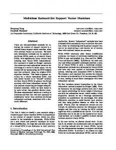
To illustrate the normalization problem of the SVMs outputs and to get some insight on possible solutions, let consider the artificial example of Figure 1. The data, partitioned into three classes, are drawn according to three Gaussian distributions with exactly the same covariance matrix and different mean vectors indicated by stars in Figure 1.

835

! ~

"'"

9

0.5

*'"

9

"

9

#~k' o'r1761769 ~ o ~ 9 ~

.'. ,~" .."

9

I'i-

,

~

il_i!

%Oo.~. o'.';~.,

"." ""

'

9

"

Oo

%,

.

9

"'"

].3k

Class 1

~! i \

0

/

-1

Class 2 \

~'~

"" : : " .

.:-., .:

: :-....

1.5

9

~' I

-2.5

~'I

-2

-1.5

I

-1

I

-0.5

Fig.

1.

A

I

I

I

I

0

0.5

1

1.5

11

2

I

2.5

3-class example.

Since the three covariance matrices are identical and the a priori probabilities are equal, the boundaries of the decision regions based on an exact Bayesian classifier are three lines intersecting in one point [7], which are represented by continuous lines on Figure 1. The 50 data of each class is linearly separable from the data of the other two classes. However, the maximal margin of a linear separator isolating Class 3 from Class 1 and 2 is much larger than the margin of the other two linear separators. Thus, when using 3 linear SVMs to solve the three dichotomies, the norm of the optimal hyperplane found by SVM algorithm is much smaller in one case than in the other two. Whenever the output class is selected as the one corresponding to the SVM with largest output, the decision region obtained is shown in Figure 1 by dashed lines, which is quite different from the optimal Bayes decision. For comparison, the dash-dotted lines (with cross-point marked by a square) correspond to the boundaries of the decision regions obtained by three linear Perceptrons trained by the Pseudo-inverse method, i.e. the linear separators minimize mean square errors [7]. This matches closely the optimal one. Two different ways of normalizing the outputs of the SVMs are also illustrated in Figure 1 and the boundaries of the corresponding decision regions are shown with dotted lines. In one case, the

836

parameters (w k, bk) of each of the K separating hyperplanes {~ I ~rwk + bk = O} are divided by the Euclidean norm of w k (the crosspoint of the boundaries is a circle). In the other case, (w k, bk) are divided by the estimate of the standard deviation of the output of the SVM (the cross-point of the boundaries is a triangle that superposes the circle).

3

S V M output normalization

The first normalization technique considered has a geometrical interpretation. When a linear classifier fk : ~d __+ {--1, +1} of the form ]k(X) = sgn(gk(w)) ----sgn(xrw k q- bk) (1) is normalized such that the Euclidean norm Ilwkll2 is 1, gk(x) gives the Euclidean distance from ~c to the boundary of fk. Non-linear SVMs are defined as linear separators in a high dimensionM space 7-/in which the input space I~d is mapped through a non-linear mapping 9 (for more details on SVMs, see for example the very good tutorial [3] from which our notations are borrowed). Thus, the same geometrical interpretation holds in 7-/. The parameter w k of the linear separator fk in 7-/of the form (1) is never computed explicitly (its dimension may be huge or infinite). But is known as a linear combination of images through 9 of the support vectors (input data with indices in N~) wk =

E

P P

P

).

(2)

p~N ~, k used in this work will thus be defined The normalization factor rrw by 1 -(-~):

~

aka~P " P~' y r

r

(3)

p ,p' 6 N ks :

E

~P'~P'~'P~'P'I((TP ~k~k~ u., ,~C P' ),

(4)

P,Pi~-Nsk

where K is the kernel function allowing an easy computation of dotproducts in 7-/.

837

One way to normalize is scaling the output of each support vector machine such that Ep[y gk(x)] = 1 The scaling factor 7rk is defined as the mean over the samples, of yPgk(xP), again estimated on the training set or on new data. Each normalization factor can also be chosen as the optimal solution of an optimization problem. The factor 7rk. minimizes the mean square error over the samples, between the normalized output 7ck,gk(x p) and the target output yP 6 { - 1 , + 1 } . Z(.

(5)

= P

whose optimal solution is (6)

4

Stacking SVMs and singlelayer perceptrons

So far, the output class is determined by choosing the maximum of the outputs of all SVMs. However, the responses of other SVMs than the winner carry also some information. Moreover, when a SVM is trained to separate one class wk from the K - 1 others, it may happen that the mean of gk varies significantly from one class to another. For example, if class w2 lies somewhere "in-between" class wl and class wa, the function g I separating class Wl from w2 and w3 is likely to have a stronger negative answer on w3 than on w2. This knowledge can be used to improve the overall recognition. A simple way to aggregate the answers of all the K SVMs into a score for each of the classes is by a linear combination. If g = (91... ,gK)m denotes the output of the system of K SVMs, the idea suggested here is to replace the former function

P -- arg max(g) by /~ = arg mkax( M g ) ,

838

where M is a K x K mixture matrix. The classical way of solving a K-class classification problem by one-per-class decomposition corresponds to using the identity mixture matrix. The technique given in Section 3 with 7ck corresponds to a diagonal M with 7ck as the diagonal elements. If sufficiently many data are available to estimate more parameters, a full mixture matrix can provide a finer way of recombining the outputs of the different SVMs. This way of stacking a set of K classifiers with a single layer neural network provides a solution to the normalization problem as long as the network (i.e. the mixture matrix M ) is designed to minimize the m e a n square error between g ( x p) and yP = { - 1 , . . . , + 1 , . . . , - 1 } . Generalizing Equation (5), we get

E ( M ) = ~--][Mg(x p) - yp]2

(7)

p

5

Numerical experiments

All the experiments reported in this section are baed on datasets of the Machine Learning repository at Irvine [10]. The values listed are pecentages of classification errors, averaged over 10 experiments. For glass and dermatology, one time 10-fold cross validation was done, while for vowel and soybean, the ten runs correspond to 5 times 2-folding. We used SVMs with polynomial kernel of degrees 2 and 3. k k database deg no normal. 71"w ~, 31.6 =h 10.3 31.9 412.3 glass 2 35.7 =h 13.5 glass 3 37.6 =h 12.8 33.3 =t= 11.4 35.7 + 10.6 3.9 + 1.9 dermatology 2 3.9 -t- 1.9 4.1 -t- 2.0 4.4 + 2.7 3.9 4- 2.7 dermatology 3 3.9 :t: 2.7 vowel 2 70.3 =t= 39.7 69.8 -t- 40.7 69.9 ~: 40.5 vowel 3 62.1 =h 44.5 61.4 :t: 45.4 61.8 ::h 44.9 soybean 2 71.6 4- 34.7 71.6 4- 34.8 71.6 :k 34.9 soybean 3 71.6 :k 34.8 71.4 =h 35.1 71.6 :t: 34.8

M ~39.0 + 12.5 45.2 :t: 10.8 4.2 =h 2.0 4.4 =h 2.7 24.2 + 1.6 10.5 4- 3.2 29.2 :t: 11.2 28.8 -4- 11.1

We notice that on the four datasets, the two normalization techk or using 7r,k do not improve accuracy except niques of dividing by ~rw in glass where a small improvement is seen. Using stacking with a linear model on vowel and soybean significantly improves accuracy

839

which demonstrates the useful effect of postprocessing SVM outputs. Overtraining certainly explains the deterioration of this stacking approach on glass, as this is a very small dataset. One can use more sophisticated learners instead of a linear model whereby accuracy can be further improved. One interesting possibility is to use another SVM to combine the outputs of the first layer SVMs. We are currently experimenting with larger databases, other types of kernels and other combining strategies and we are expecting to have more extensive support of this approach in the near future.

6

Robust decomposition/reconstruction schemes

Lately, some work has been devoted to the issue of decomposing a K-class classification problem into a set of dichotomies. Note that all the research we are referring to was carried out independently of the method used to learn the dichotomies, and consequently all the techniques can be applied right away with SVMs. The one-per-class decomposition scheme can be advantageously replaced by other schemes. If there are not too many classes, the so called pairwise-coupling decomposition scheme is a classical alternative in which one classifier is trained to discriminate between each pair of classes, ignoring the other classes. This method is certainly more efficient than one-per-class, but it has two major drawbacks. First, the number of dichotomies is quadratic in the number of classes. Second, each classifier is trained with data coming from two classes only, but in the using phase, the outputs for data from any classes are involved in the final decision [11]. A more sophisticated decomposition scheme, proposed in [6,5], is based on error-correcting code theory and will be referred to as ECOC. The underlying idea of the ECOC method is to design a set of dichotomies so that any two classes are discriminated by as many dichotomies as possible. This provides robustness to the global classifier, as long as the errors of the simple classifiers are not correlated. For this purpose, every two dichotomies must also be as distinct as possible. In this pioneering work, the set of dichotomies was designed a priori, i.e. without looking at the data. The drawback of this approach

840

is that each dichotomy may gathers classes very far apart and thus is likely hard to learn. Our contribution to this field [8] was to elaborate algorithms constructing the decomposition matrix a posteriori, i.e. by taking into account the organization of the classes in the input space as well as the classification method used to learn the dichotomies. Thus, once again, the approach is immediately applicable with SVMs. The algorithm constructs the decomposition matrix iteratively, adding one column (dichotomy) at a time. At each iteration, it chooses a pair of classes (wk,c0k,) at random among the pairs of classes that are so far the less discriminated by the system. A classifier (e.g. a SVM) is trained to separate wk from wk,. Then, the performance of this classifier is tested on the other classes and a class wl is added to the dichotomy under construction as a positive (resp. negative) class, if a large part of it is classified as positive (resp. negative). The classifier is finally retrained of the augmented dichotomy. The iterative construction is complete, either if all the pairs of classes are sufficiently discriminated or when a given number of dichotomies is reached. Although each of these general an robust decomposition techniques are applicable to SVMs and must be in any case preferred to the one-per-class decomposition, they do not solve the normalization problem. When choosing a general decomposition scheme composed of L dichotomies providing a mapping from the input space J2 into { - 1 , +1} L or ]~L, one also has to select a mapping rn : IRL --+ 11~K, called the reconstruction strategy, on which the arg maxk operator will finally be applied. Among the large set of possible reconstruction strategies that have been explored in [9], one distinguishes the a p r i o r i reconstructions from the a posteriori reconstructions. In the latter, the mapping rn can be basically any classification technique (neural networks, decision trees, nearest neighbor, etc.). It is learned from new data and thus, it solves the normalization problem. Reconstruction mappings rn composed of L SVMs have also been investigated in [9] and provided excellent results, especially for degree 2 and 3 polynomial kernels. Note that in this case, the normalization problem occurs again at the output of the mapping rn and in our

841

experiments we cope with it using the normalization factors 7rw, l l 1,...,L. When the decomposition scheme is constructed iteratively by the algorithm described above and the reconstruction mapping is based on SVMs, a considerable amount of computation time can be saved as follows. At the end of each iteration constructing a new dichotomy, the mapping m must be elaborated based on the current number of dichotomies, say L, in order to determine (in the next iteration) the pair of classes ( w k , w k , ) for which the global classifier is doing the worse confusion. But the optimal mapping m : ]I~ L ---+ ]I~ K have some similarities with m ' : I~ n - 1 --+ I~ I~ constructed at the previous iteration. It has been observed that the quadratic program determining the 1~hSVM of the mapping m is solved much faster when initialized with the optimal solution (the a~s indicating the support vectors and their weights) of the quadratic program corresponding to the l ~hSVM of the mapping m ~.

7

Conclusions

In this paper, the problem of normalizing the outputs of several SVMs, for the sake of comparison, is highlighted. Different normalization techniques are proposed and experimented. More elaborated methods allowing the usage of binary classifiers for the resolution of multi-class classification problems are briefly presented. The experimentation of these approaches with SVMs as well as with other learning techniques is a large scale ongoing work and will be presented in the final version of this paper. References 1. B. E. Boser, I. M. Guyon, and V. N. Vapnik. A training algorithm for optimal margin classifiers. In Proceedings of the Conference on Learning Theory, COLT'92, pages 144-152, 1992. 2. L. Breiman, J. Olshen, and C. Stone. Classification and Regression Trees. Wadsworth International Group, 1984. 3. C. Burges. A tutorial on support vector machines for pattern recognition. Data Mining and Knowledge Discovery, to appear, available at h t t p : / / s v m . r e s e a r c h , b e l l - l a b s , com/SVMdoc, html. 4. C. Cortes and V.Vapnik. Support vector network. Machine Learning, 20:273-297, 1995.

842

5. Thomas G. Dietterich and Ghulum Bakiri. Solving multiclass learning problems via error-correcting output codes. Journal of Artificial Intelligence Research, 2:263286, 1995. 6. T. G. Dietterich and G. Bakiri. Error-correcting output codes : A general method for improving multiclass inductive learning programs. In Proceedings of AAAI-91, pages 572-577. AAAI Press / MIT Press, 1991. 7. R. O. Duda and P. E. Hart. Pattern Classification and Scene Analysis. John Wiley & Sons, New York, 1973. 8. Eddy Mayoraz and Miguel Moreira. On the decomposition of polychotomies into dichotomies. In Douglas H. Fisher, editor, The Fourteenth International Conference on Machine Learning, pages 219-226, 1997. 9. Ana Merchan and Eddy Mayoraz. Combination of binary classifiers for multi-class classification. IDIAP-Com 02, IDIAP, 1998. paper 22 in the Proceedings of Learning'98, Madrid, September 98, http://learn98, tsc. uc3m. es/~learn98/papers/abst ract s.

10. C. J. Merz and P. M. Murphy. UCI repository of machine learning databases. Machine-readable data repository h t t p ://www. ics .uci. edu/~mlearn/mlrepository.html, Irvine, CA: University of California, Department of Information and Computer Science, 1998. 11. Miguel Moreira and Eddy Mayoraz. Improved pairwise coupling classification with correcting classifiers. IDIAP-RR 9, IDIAP, 1997. To appear in the Proceedings of the European Conference on Machine Learning, ECML'98. 12. J. R. Quinlan. Induction of decision trees. Machine Learning, 1:81-106, 1986. 13. B. Schrlkopf, C. Burges, and V. Vapnik. Extracting support data for a given task. In U. M. Fayyad and R. Uthurusamy, editors, Proceedings of the First International Conference on Knowledge Discovery and Data Mining, pages 252-257. AAAI Press, 1995. 14. V. N. Vapnik. The Nature of Statistical Learning Theory. Springer, New York, 1995.