Multiple Linear Regression to Improve Prediction Accuracy in WSN Data Reduction Carlos Giovanni Nunes de Carvalho, Danielo Gonçalves Gomes and José Neuman de Souza Group of Computer Networks, Software Engineering and Systems (GREat) Federal University of Ceará (UFC) Fortaleza, Brazil
[email protected],{danielo,
[email protected]}
Nazim Agoulmine LRSM/IBIC Laboratory University of Evry Val d’Essonne France
[email protected]
Abstract— Simple linear regression is usually used for WSN data reduction. The mechanism is concerned about energy consumption, but neglects the prediction accuracy. The prediction error from it is often ignored and inconsistencies are forwarded to the user application. This paper proposes to use a method based on multiple linear regression to improve prediction accuracy. The improvement is achieved by multivariate correlation of readings gathered by sensor nodes in field. Tests show that our solution outperforms some current solutions adopted in the literature.
correlation of only one variable to be predicted (named dependent or response variable, e.g. temperature) and only one variable to predict the dependent variable (named independent or explanatory variable, e.g. time/epoch). However, prediction accuracy increases when more than one independent variable is used and they are strongly correlated. Furthermore, the time variable is not the more correlated variable with others variables such as temperature, humidity and light. Thus, the prediction adopted by current solutions, is sometimes not accurate.
Keywords- Prediction accuracy, wireless sensor network, multivariate correlation, data reduction, linear regression functions
We propose a method that performs prediction based on multivariate correlation. In our method, we take into account the correlation between two readings of data gathered by the sensor node and the time variable/epoch. Our method is different from current works which use the correlation between one variable gathered and the time variable.
I.
INTRODUCTION
Sensors can be used in a lot of applications such as event detection, location, monitoring and control. Among these applications, environment monitoring is a very common scenario. Therefore, data gathering is periodical, generating a large amount of data flow in the network. The data flow is a problem in WSN due to energy consumption [9]. In this scenario, the sensor nodes frequently send the same information gathered from a specific area. The overlapping of information sent to the sink causes waste of energy, which decrease the network lifetime. The problem tends to worsen according to the number of nodes deployed (scalability), because data communication is responsible for most of the energy consumption in WSN [2]. The correlation between the data gathered by sensor node and its neighbors, as well as the correlation between the data gathered by the sensor node itself over a given time [9] is important for efficient protocols. They are known as spatial and temporal correlation. When more than one variable in the correlation is taken into account, it was named multivariate correlation. Prediction of data purposely not sent to the sink in order to reduce traffic, is a technique which has been adopted in the literature [5]. It helps reducing the overall energy consumption of the network. An algorithm is embedded within the sensor node to calculate the coefficients of a linear regression function. These coefficients are named β and α, and represent a sequence of variable samples gathered by the sensor, such as temperature. This approach usually takes into account the The authors would like to thank the Brazilian funding agencies FAPEPI (PhD Scholarship) and CNPq for their financial support.
978-1-4577-1792-5/11/$26.00 ©2011 IEEE
II.
METODOLOGY
Tree-based routing protocol to forward the data flow to the sink node is used, an approach similar to the one adopted, by Li et al. [3]. Nevertheless, to avoid spatial overlapping in our proposal, each sensor node checks whether there is a degree of multivariate correlation between the packets previously sent by its neighbors. This is done before each sensor node sends the linear regression coefficients to the sink. Moreover, multiple linear regression prevents temporal overlapping in the same sensor node. In this paper, simulations with simple and multiple linear regression functions were carried out to evaluate the prediction solution in two phases: 1) the correlation degree of the variables gathered from the sensor node is measured to decide which variable will be the independent one. Here in this paper, the Pearson’s coefficient (r) in a real data trace indicates the strength of a linear relationship between two variables, e.g. if the variables area independent, the Pearson’s coefficient is zero; 2) to evaluate prediction accuracy, the sensor nodes run linear regression functions. An original application to data gathering without any prediction mechanism was developed. This application emulates a real gathering of temperature, humidity and light data. Then, the original version of this application is compared to two modified versions that use
simple linear regression and one that uses multiple linear regression. Prediction accuracy performance is evaluated by means of Residual Sum of Squares (SSerr) and coefficient of determination (R2) [1]. They are used to compare both versions using simple linear regression and version using multiple linear regression. SSerr is the sum of power of prediction errors for each dependent variable using simple or multiple linear regression. R2 represents the improvement of the sum of the power of prediction errors. III.
RELATED WORK
Some works [3][4][8] have showed the feasibility of the use of spatial and temporal correlation to optimize the communication protocols in WSN. They use algorithms embedded within motes, in distributed or centralized way, to reduce data transmission to the sink. These techniques reduce energy consumption and consequently increases the network lifetime. Xu and Lee [10] propose a localized prediction mechanism based on object tracking that reduces energy consumption due to hierarchy topology. Matos et al. [5] propose simple linear regression to reduce data generated by sensor nodes which gather temperature from the external environment. They compare the prediction accuracy performance of the simple linear regression to prediction based on the average. The difficulty lies on the fact that prediction accuracy based on simple linear regression depends on one variable, which in many situations is not correlated with each other. The time variable is usually less correlated than other variables that are being gathered on field, such as temperature, humidity or light. Therefore, prediction errors tend to be higher, i.e., less accurate. That paper is the closest to our proposed solution, but it performs prediction of user’s queries, instead of constantly performing prediction of stream. Seo et al. [6] carried out evaluations in some techniques for reducing the multivariate data flow. These techniques are based on wavelet, sampling, hierarchical clustering and Singular Value Decomposition – SVD. Silva et al. [7] reduces data dimensionality gathered by sensor nodes. The authors used Principal Component Analysis – PCA as reduction technique in an air quality monitoring application. However, there is no concern for multivariate spatial correlation. Also, there are few details about the solution operation, mainly about the result error from the dimensionality reduction procedure. Multivariate spatial and temporal correlation is key to solve problems of prediction accuracy through data reduction techniques. The works found in the literature have superficially addressed their implementation. Our paper has the advantage of performing correlation analysis of variables gathered by sensor nodes before the prediction is implemented. Also, the effects of using prediction based on multivariate spatial and temporal correlation in WSN were checked. IV.
BACKGROUND
Many sensor nodes deployed on field are able to perform monitoring of more than one variable, which we named multisensor. Moreover, those variables are usually strongly correlated. In this section we describe two techniques found in the literature which are used in the conception of our method.
To the best of our knowledge, we did not find any paper that uses multiple linear regressions to perform prediction and which also uses Euclidian distance. But, we found papers such as Skordylis et al. [8] which use a technique adopted for spatial correlated data reduction by Pearson’s coefficient (r). Also, we found a paper such as Matos et al. [5] which uses a technique adopted for temporal correlated data reduction by simple linear regression. A. Pearson’s coefficient The Pearson’s coefficient (Equation 1) is used for works such as [8] to identify the spatial correlation of the same variable between two sensor nodes. It can also be used to identify the correlation between two variables of the same sensor node. In our work, it is used to figure out the correlation degree (weak or strong) between variables gathered by sensor nodes on field. ∑ ,
∑
∑
(1)
represents the relationship between two where , and , to be compared in terms of unidimensional vectors their correlation. They contain samples history of two ,…, and ,…, , where variables, 1, … , and is the number of samples. and represent the average of samples of each variable vector. When the coefficient r is close to bounds (1 or -1), the correlation between two vectors is strong. Thus, we can calculate the spatial and temporal correlation of the readings of just one variable between two neighbor sensor nodes [8]. The problem is that we cannot calculate the multivariate spatial correlation, which is necessary for our solution. But, we can build a table which determines how much one variable is related to another. The correlation table for variables from real data trace is showed in the next section. The coefficient r is used to identify what variable is more correlated to another in our solution. This more correlated variable was used to calculate β and α coefficients of the multiple linear regression and also for recovery in the sink to which the data was not sent. B. Simple linear regression The current solutions of data reduction by linear regression are performed by using simple linear regression based on the least squares (Equation 2 and Equation 3), as applied by Matos et al. [5]. In that case, each sensor node calculates β and α coefficients by using one variable, usually the epoch/time. Then, the sensor node sends its β and α coefficients to the sink, instead of sending the readings. The advantage of that solution is that energy consumption is reduced, but on the other hand, the prediction is sometimes not accurate. ∑
β
(2)
∑
α
β
(3)
where β represents a constant that is multiplied by the value of each independent variable. α is a constant added to the previous multiplication, resulting in the predicted value. and are two unidimensional vectors, which respectively represent samples history of the independent and dependent variables, with , … , and , … , , where 1, … , and is the number of samples. and represent the average of samples of each vector. Two application versions based on univariate correlation (simple linear regression based on the least squares) were developed and compared to other version, which is based on multivariate correlation (our solution). The β and α coefficients are calculated according to Equation 2 and Equation 3. α
β
•
Step 2: Each sensor node calculates the β and α coefficients of the multiple linear regression function when they reach the maximum storage threshold previously defined.
•
Step 3: Each sensor node checks its table of β and α coefficients received from its neighbor sensor nodes by broadcast, before sending β and α coefficients to the sink.
•
Step 4: If the values generated by the sensor node already have been sent earlier to a neighbor sensor node, the sensor node drops the β and α coefficients calculated by it. Then, it sends a special packet of reduced size, named correlation packet. This packet advertises that the sensor node is correlated to another neighbor sensor node.
•
Step 5: If β and α coefficients have not been sent by another neighbor sensor node yet, they are sent to its parent node until the sink is reached.
•
Step 6: After Step 5, the sensor node also sends the sequence of variable readings which is used as independent variable. It is worth mentioning that this variable was found by using Pearson's coefficient (Equation 2). In our experiment the variable is the temperature.
•
Step 7: When β and α coefficients reach the sink, they are used in the multiple linear regression function to predict the readings which have not been sent. Moreover, these β and α coefficients are stored for later use by the correlation packets (Step 4).
•
Step 8: Similarly, when the correlation packet arrives at the sink, it uses β and α coefficients previously stored (Step 7).
(4)
and represent one unidimensional vector, where which respectively contain the values of the predictions made by one dependent variable and samples history of one ,…, and independent variable . ,…, , where 1, … , and is the number of samples. β and α respectively represent the coefficients calculated by Equation 2 and Equation 3. The β and α coefficients are calculated by each sensor node and are used at the moment of arrival at the sink, according to Equation 4. In our solution, Equation 4 is extended due to multivariate correlation. We used multiple linear regression instead of simple linear regression. Then, in the next section, we describe how to calculate the β and α coefficients to perform our method. V.
A. Steps of our proposal • Step 1: Each sensor node stores a fixed number of samples of gathered readings from all the variables.
PROPOSED SOLUTION
The purpose of our paper is to apply the multivariate correlation method to improve prediction accuracy on WSN data reduction. The data reduction is performed by multiple linear regressions which calculate its β and α coefficients. Each sensor node sends β and α coefficients to the sink, instead of sending all data gathered by the sensor node on field. Given this: 1) prediction of consecutive readings by multiple linear regression is performed in each sensor node, preventing multivariate temporal overlapping; 2) each sensor node calculates the β and α coefficients, then sends them to the sink, instead of all the readings gathered on field; 3) If Euclidean distance detects the presence of multivariate spatial overlapping, the packet is dropped. Therefore, we prevent the same information to be sent by multiple neighbor sensor nodes; and 4) the not sent data recovery is made by the sink. Main contributions of this paper are: 1) to start a new discussion about prediction accuracy in environmental monitoring, which includes the correlation between variables gathered such as temperature, humidity and light; 2) to show that is possible to deploy more accurate prediction solutions through the multivariate correlation method; and 3) to present the challenges and shows in details the steps required to deploy this solution for data reduction with prediction approach by multiple linear regression.
B. Multivariate spatial correlation The spatial correlation can be exploited to optimize data communication to the sink and between neighbor sensor nodes [4][8][9]. It happens due to overlapping of data being sent to the sink by several sources from high density network [9]. We use the Euclidean distance (Equation 5) to determine the multivariate spatial correlation between two multidimensional vectors, instead of using Pearson’s coefficient. The Euclidian distance shows how close a multidimensional vector is to other. ,
∑
(5)
represents the correlation between two where , multidimensional vectors of dimension and 1, … , , to be compared in terms of their correlations. Each vector contains the values of β and α coefficients of each gathered variable by sensor node and its neighbor sensor node with ,…, and ,…, .
The smaller the Euclidean distance, higher the correlation between two vectors. Thus, we can compare β and α coefficients of the multiple linear regression generated from consecutive readings gathered by a sensor node to β and α coefficients from its neighbor sensor nodes at a given time. If the Euclidian distance is close to 0 (zero), then it means that a packet with the same content was previously sent by any other neighbor sensor node (Step 4). In our proposed solution, the sensor node detects if there is multivariate spatial correlation between itself and its neighbor node by tree-based routing. This is similar to the compression mechanism adopted by Li et al. [3]. The sensor node checks the relationship degree of β and α coefficients by calculating the value of (Equation 5). It eliminates the overlapping , of information between neighbor sensor nodes. Thus, some sensor nodes do not send data packets at a given time. Thereby, it reduces the broadcast between neighbor sensor nodes and also the data forwarded by the relays. C. Multivariate temporal correlation The temporal correlation happens due to the fact that the sensor node gathers correlated data from one or more variables at a given time. It is observed in the nature of physical phenomena [9]. The simple linear regression function is able to work over temporal correlation, but it is not able to work over the multivariate temporal correlation (more than one variable). In our solution, we use multiple linear regression function to work over the multivariate correlation.
β
XX
X Y with β
β β
(6)
β where β represents the vector of constants which are multiplied by each value of the independent variable. But, we α for simplicity and compatibility with β and α use β coefficients of the simple linear regression (previous section). is one multidimensional vector, which represents the samples history of the independent variable (Step 1), together with its transpose vector . is one unidimensional vector, which represents the samples history of the dependent variable (Step 1). Our data reduction solution occurs in a distributed way, where each sensor node calculates β and α coefficients from the multiple linear regression (regression based on the least squares) function (Step 2). Then, it only sends β and α if there is no multivariate spatial correlation with other neighbor sensor node. Β and α coefficients are not calculated by the simple linear regression as the amount of independent variables is greater. The multiple linear regression is described, according to Equation 6. D. Data recovery The last step occurs in the sink, which receives β and α coefficients or the correlated packet. Thereafter, the predictor calculates the values of the missing readings based on β and α coefficients (Step 7) by the multiple linear regression function (Equation 7). But, if the correlated packet arrives at the sink, it
uses β and α coefficients of the correlated sensor node (Step 8), advertised by the packet and previously recorded (Step 7) from a neighbor sensor node. β
β
,…, β
(7)
where represents one unidimensional vector, which contains the values of predictions made for one dependent represents the multidimensional vector, variable and which contains values history of the samples from more than ,…, and one independent variable . ,…, , with 1, … , , where is the number of samples, and 1, … , , where is the dimension of the vector . β and α respectively represent the coefficients calculated using Equation 6. As a reminder β α due to compatibility with the notation of β and α coefficients which is used in this paper. VI.
EXPERIMENTS AND RESULTS
The main goal of our proposed solution is not to reduce energy consumption compared to the current works based on simple linear regression. Although our solution to spend twice the amount of energy compared to simple linear regression, it is still cheaper than the application without data reduction. Tests were run in Tossim simulator involving simple linear regression function (one dependent variable and one independent variable) and multiple linear regression function (one dependent variable and more than one independent variable). A. Application versions The performance evaluation was done through four application versions, which we used to simulate and compare multiple linear regression to simple linear regression and of the original version of a monitoring application. This monitoring application simulates the gathering of three variables from the environment, as temperature, humidity and light. The TinyOS 2.x provides for default, packets up to 28 bytes to be sent by applications of sensor nodes. Therefore, we only use the amount of fields with their respective sizes needed to fit the maximum acceptable size. We created four application versions to achieve the simulations, where: •
First version (a.k.a Original): sends temperature, humidity and light readings periodically every 1024 clock shots from the sensor node, without performing prediction. This version was created to serve as base for us to verify the energy consumption in the later versions, which use prediction for data reduction. It is the original application (without prediction). For this version there is only one type of application packet of 20 bytes containing readings of data gathered of the temperature, humidity and light variables. In addition, this packet contains information to be manipulated by the network layer.
•
Second version (a.k.a SimpleCount): modified version of the original application through of a simple linear regression function. It sends only β and α coefficients
for each dependent variable, without sending any reading. It uses a counter (time variable) as the independent variable to predict the temperature, humidity and light variables. This version is based on the method proposed by current works as Matos et al. [5]. In this version, we created two types of application packets: one packet of 20 bytes containing β and α coefficients calculated for each dependent variable; and one reduced size packet of 10 bytes to send the message that the sensor node is spatially correlated to a neighbor sensor node. Moreover, the two packets above containing information to be manipulated by the network layer. •
•
Third version (a.k.a SimpleTemperature): modified version of the second version through a simple linear regression function using the temperature as independent variable, instead of time variable. It sends reading samples of the temperature variable and β and α coefficients for each dependent variable (except temperature) to predict the dependent variables humidity and light. The temperature was chosen as independent variable due to the results obtained from coefficient r, which can be seen later in the next section. Three types of application packets were created in this version: one packet of 20 bytes containing β and α coefficients calculated for each dependent variable (except the temperature variable); one reduced size packet of 10 bytes to send the message that the sensor node is spatially correlated to a neighbor sensor node; and one packet of 18 bytes containing 10 readings of temperature in sequence to be used in the prediction of the humidity and light variables. In addition, the three packets above containing information to be handled by the network layer. The temperature variable is sent in sequence in a same packet, because it is not more predicted by the sink and is also used to predict the other two variables. Fourth version (a.k.a. Multiple): modified version of the original application through a multiple linear regression function, using counter and temperature as independent variables. Our proposed method is based on this version. It sends reading samples of temperature and β and α coefficients for each dependent variable (except temperature) with , , where . It predicts the dependent light and humidity variables. Three types of application packets were created in this version: one packet of 20 bytes containing β and α coefficients calculated for each dependent variable (except temperature), with , , where ; one reduced size packet of 10 bytes to send the message that the sensor node is spatially correlated to a neighbor sensor node; and one packet of 18 bytes containing 10 temperature readings in sequence to be used in the prediction of the humidity and light variables. In addition, the three packets above containing information to be manipulated by the network layer. The temperature variable is sent in sequence in a same packet as in the third version.
B. Scenarios We simulated six different scenarios 30 times each. The scenarios have all four application versions and the number of nodes ranges from 4 to 100. All results obtained from experiments have confidence interval of 95%. We observed from the trace that the light variable presented different values. Also, it was verified that the type of topology and density influenced the results. Then, in order to evaluate the performance, scenarios with the following characteristics were used: •
Scenario 1: Gathered readings with the values of the light variable constant, topology in grid and network density with one sensor node every 5 meters.
•
Scenario 2: Gathered readings with the values of the light variable not constant, topology in grid and network density with one sensor node every 5 meters.
•
Scenario 3: Gathered readings with values of the light variable not constant, random topology and network density ranging according to the number of sensor nodes.
•
Scenario 4: Gathered readings with values of the light variable constant, random topology and network density ranging according to the number of sensor nodes.
•
Scenario 5: Gathered readings with values of the light variable not constant, random topology and fixed network density.
•
Scenario 6: Gathered readings with values of the light variable constant, random topology and fixed network density.
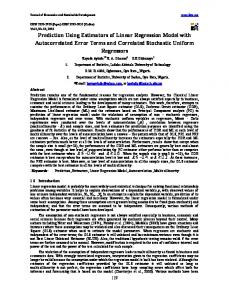
C. Analysis of correlation between gathered variables Initially the level of correlation between gathered variables by sensor nodes was found to define which variable would be the best choice as independent variable. This analysis of correlation was run through Pearson's coefficient (r) (Equation 1) on a real trace of Intel Berkeley Research (http://db.csail.mit.edu/labdata/labdata.html). The coefficient r results (Table I) show that there is a greater correlation between the temperature variable and other variables gathered by the sensor nodes (such as humidity and light) than with the time variable. The time variable is usually used by prediction solutions of WSN found on the literature. D. Performance evaluation We developed and embed all four application versions within the sensor nodes in the Tossim. Then, we measured the performance of prediction accuracy to reveal how much better our solution is compared to currents works. It simulates the gathering of temperature, humidity and light without prediction. SSerr and R2 results from prediction of the light (Figure 1 – Appendix) show that there are different behaviors in the scenarios where the light variable is irregular.
TABLE I. RESULTS OF THE CORRELATION ANALYSIS Temperature Humidity Light Time
Temperature 1.0000 -0.7987 0.4550 -0.2681
Humidity -0.7987 1.0000 -0.2489 0.1987
Light 0.4550 -0.2489 1.0000 -0.1807
VII. CONCLUSIONS Time -0.2681 0.1987 -0.1807 1.0000
As per previous section, the gathered readings of the light variable in the trace are irregular, sometimes they are constant and sometimes they are not constant. But, SSerr and R2 results from prediction of humidity (Figure 2 – Appendix) show for all scenarios that the lowest prediction accuracy was obtained when we compared simple linear regression based on the time and temperature variables as explanatory variable. The best prediction accuracy was obtained when multiple linear regression was used. The multiple linear regression function does not work properly in the presence of low correlation between variables. On the other hand, the multiple linear regression remains the best choice for predicting of the humidity variable. The performance evaluation of prediction accuracy was repeated to analyze the behavior of our solution. When we increase the samples amount, energy consumption decreases, SSerr increases and improvement decreases. But, WSN cannot spend much energy, thus Scenario 6 was simulated again, due to the fact that it had better performance results among the other scenarios. The samples amount ranged from 6 (six), 8 (eight) and 10 (ten), which we respectively named Scenario 6C, Scenario 6B and Scenario 6A. Then, the improvement of humidity for the application version 4 (multiple linear regression) decreased from 0.995868 to 0.978811 (Figure 3a – Appendix) and the SSerr of humidity increased from 0.021840 to 0.203488 (Figure 3b – Appendix). Note also that the application version 4 had always better results than the others versions. The results for light are a little bit different than the results for humidity but had the same behavior. The improvement of the light for application version 4 (multiple linear regression) decreased from 0.999752 to 0.974384 (Figure 4a – Appendix) and the SSerr of the light increased from 0.000384 to 0.054342 (Figure 4b – Appendix). E. Light results The results for improvement of the prediction of the light variable show the drawback of multiple linear regression. Where there is no correlation between the variables, prediction accuracy decreases or does not work properly. Table II and Table III (Appendix) show more details of the results of SSerr and R2. Figure 5 (Appendix) shows epochs from a collecting day where the correlation between the variables is low. Note that in epochs ranging from 3550 to 4900, the light variable increases a lot. Consequently, the simple and multiple linear regressions tend to worsen prediction accuracy. This explains some abnormal results when we used the light variable as independent variable.
Several sensor boards are able to monitor more than one variable (multisensor), adding new challenges, such as increasing precision by reducing prediction error. So, we propose a method to improve prediction accuracy on WSN data reduction by applying multivariate spatial and temporal correlation. We conducted experiment simulations involving simple and multiple linear regression functions to assess our prediction solution. Results of SSerr and R2 show that multivariate correlation method outperforms current methods of prediction accuracy. Therefore, we conclude that the solutions currently adopted are more susceptible to errors than our proposal. Usually they use simple linear regression based on the time variable as independent variable. Although multiple linear regression spends a little more energy than simple linear regression in data communication, it may be the best choice. ACKNOWLEDGMENT Carlos Giovanni would like to thank the State University of Piauí (UESPI) to support as professor of Computer Science. REFERENCES [1]
Hair, J., Black, W., Babin, B., and Anderson, R (1998). Multivariate Data Analysis. Prentice Hall. [2] Koshy, J., Wirjawan, I., Pandey, R., and Ramin, Y. (2008). Balancing computation and communication costs: The case for hybrid execution in sensor networks. Ad Hoc Networks, 6(8):1185 – 1200. Energy Efficient Design in Wireless Ad Hoc and Sensor Networks. [3] Li, J., Deshpande, A., and Khuller, S. (2010). On computing compression trees for data collection in wireless sensor networks. In Proceedings of the 29th conference on Information communications, INFOCOM’10, pages 2115–2123, Piscataway, NJ, USA. IEEE Press. [4] Liu, C., Wu, K., and Pei, J. (2007). An energy-efficient data collection framework for wireless sensor networks by exploiting spatiotemporal correlation. Parallel and Distributed Systems, IEEE Transactions on, 18(7):1010 –1023. [5] Matos, T. B., Brayner, A., and Maia, J. E. B. (2010). Toward in-network data prediction in wireless sensor networks. In Proceedings of the 2010 ACM Symposium on Applied Computing, SAC ’10, pages 592–596, New York, NY, USA. ACM. [6] Seo, S., Kang, J., and Ryu, K. H. (2005). Multivariate stream data reduction in sensor network applications. In EUC Workshops’05, pages 198–207. [7] Silva, O., Aquino, A., Mini, R., and Figueiredo, C. (2009). Multivariate reduction in wireless sensor networks. In Computers and Communications, 2009. ISCC 2009. IEEE Symposium on, pages 726– 729. [8] Skordylis, A., Guitton, A., and Trigoni, N. (2006). Correlation-based data dissemination in traffic monitoring sensor networks. In Proceedings of the 2006 ACM CoNEXT conference, CoNEXT ’06, pages 42:1–42:2, New York, NY, USA. ACM. [9] Vuran, M. C., Akan, O. B., and Akyildiz, I. F. (2004). Spatio-temporal correlation: theory and applications for wireless sensor networks. Comput. Netw., 45:245–259. [10] Xu, Y. and Lee, W.-C. (2003). On localized prediction for power efficient object tracking in sensor networks. In Distributed Computing Systems Workshops, 2003. Proceedings. 23rd International Conference on, pages 434 – 439.
APPENDIX – FIGURES AND TABLES
(a)
Improvement for light
(b)
SSerr for light
Figure 1 Improvement and SSerr of the prediction performed by application versions for the variable light.
(a)
Improvement for humidity
(b)
SSerr for humidity
Figure 2 Improvement and SSerr of the prediction performed by application versions for the variable humidity.
(a)
Improvement for humidity
(b)
SSerr for humidity
Figure 3 Improvement and SSerr of the prediction performed by application versions for the variable humidity ranging sample amount (Scenario 6A – ten samples, Scenario 6B – eight samples and Scenario 6C – six samples).
(a)
Improvement for light
(b)
SSerr for light
Figure 4 Improvement and SSerr of the prediction performed by application versions for the variable light ranging sample amount (Scenario 6A – ten samples, Scenario 6B – eight samples and Scenario 6C – six samples).
Figure 5 Epochs from a collect day where the variable light is less correlated with the variables temperature and humidity. TABLE II. PERFORMANCE RESULTS OF THE SSERR AND R2 FROM ALL VERSIONS IN SCENARIOS 1, 4 AND 6
Temperature Humidity Light
Count (Time) Version 2 SSerr R2 0.210300 0.296891 9.355700 0.025813 2.121380 0.000000
Independent variable Temperature Version 3 Sserr R2 2.033940 0.788210 0.073135 0.965525
Count and Temperature Version 4 SSerr R2 0.203488 0.978811 0.054342 0.974384
TABLEIII. PERFORMANCE RESULTS OF THE SSERR AND R2 FROM ALL VERSIONS IN SCENARIOS 2, 3 AND 5
Temperature Humidity Light
Count (Time) Version 2 SSerr R2 10.321800 0.290535 4.964100 0.476813 140.150060 0.869629
Independent variable Temperature Version 3 Sserr R2 8.583820 0.095316 794.135000 0.261311
Count and Temperature Version 4 SSerr R2 0.185308 0.980470 1075.060000 0.000000