A Multiple Linear Regression Model for Tropical ... - Semantic Scholar

atmosphere Article

A Multiple Linear Regression Model for Tropical Cyclone Intensity Estimation from Satellite Infrared Images Yong Zhao 1,2 , Chaofang Zhao 1,2, *, Ruyao Sun 1 and Zhixiong Wang 2 1

2

*

Department of Marine Technology, College of Information Science and Engineering, Ocean University of China, Qingdao 266100, China; [email protected] (Y.Z.); [email protected] (R.S.) Ocean Remote Sensing Institute, Ocean University of China, Qingdao 266100, China; [email protected] Correspondence: [email protected]; Tel.: +86-532-6678-2949

Academic Editor: Jong-Jin Baik Received: 22 January 2016; Accepted: 7 March 2016; Published: 11 March 2016

Abstract: An objectively trained model for tropical cyclone intensity estimation from routine satellite infrared images over the Northwestern Pacific Ocean is presented in this paper. The intensity is correlated to some critical signals extracted from the satellite infrared images, by training the 325 tropical cyclone cases from 1996 to 2007 typhoon seasons. To begin with, deviation angles and radial profiles of infrared images are calculated to extract as much potential predicators for intensity as possible. These predicators are examined strictly and included into (or excluded from) the initial predicator pool for regression manually. Then, the “thinned” potential predicators are regressed to the intensity by performing a stepwise regression procedure, according to their accumulated variance contribution rates to the model. Finally, the regressed model is verified using 52 cases from 2008 to 2009 typhoon seasons. The R2 and Root Mean Square Error are 0.77 and 12.01 knot in the independent validation tests, respectively. Analysis results demonstrate that this model performs well for strong typhoons, but produces relatively large errors for weak tropical cyclones. Keywords: tropical cyclone; intensity; satellite infrared image; northwestern pacific; linear regression

1. Introduction Tropical Cyclones (TCs) are some of the most damaging natural hazards [1]. The intensity (here refers to the maximum sustained wind) is generally used as a main indicator for quantifying the damage potential of TCs. Because it is difficult to obtain direct in-situ measurements of TC intensity [2], satellite remote sensing, especially geostationary meteorological satellite (GMS) remote sensing, has been heavily relied upon in related studies and operational forecasts. On the one hand, GMS has higher temporal and spatial resolution compared to polar satellite microwave remote sensing [3–5] and air reconnaissance [6–8]. On the other hand, GMS could cover the vast tropical ocean continually, and thereby provide valuable datasets concerning the genesis, track, intensity and other well-concerned information about TCs throughout their life cycles. The Northwestern Pacific Ocean (NWP), which is characterized with frequent cyclone activities, is heavily dependent on GMS for TC intensity estimation and forecast [3,9,10]. During the beginning years (1970s) of satellites, Dvorak summarized previous research [11,12] and proposed a comprehensive pattern recognition technique for tropical cyclone (TC) intensity estimation from satellite imagery, which is known as Dvorak Technique (DT) [13,14]. However, DT depends on experts’ experience, and therefore is subjective and time intensive. Several revisions of the DT technique were developed during the later decades. The Objective Dvorak Technique (ODT) [15]

Atmosphere 2016, 7, 40; doi:10.3390/atmos7030040

www.mdpi.com/journal/atmosphere

Atmosphere 2016, 7, 40

2 of 17

recognized patterns in satellite imagery using computer-based algorithm, and created a look-up table. The shortcoming of ODT is that centers of TCs are determined either manually or with the aid of external resources [16]. The more recently developed Advanced Dvorak technique (ADT), which is regarded as the latest version of DT method, advances the original Dvorak technique through modifications based on rigorous statistical and empirical analysis [17,18]. Despite the continual development of the DT method, all versions of DT technique (except for ADT) estimate TC intensity based on cloud features and patterns recognition. Apart from the DT method, some other techniques have also been developed. Mueller (2006) used geostationary IR data to estimate wind field structure of TCs through estimates of radius of maximum wind (RMAX)and wind at 182 km (V182) with 405 cases from the 1995–2003 Atlantic and Eastern Pacific typhoon seasons [19]. Chao (2011) made use of both IR and visible satellite images to estimate TC rotation speed and then sought to predict TC wind intensity using estimated rotation speeds at the 130–260 km ring [10]. Fetanat (2013) proposed a new technique for TC intensity estimation using the spatial feature analogs in satellite imagery. The technique was testified as on par with other objective techniques [20]. Zhuge (2015) combined information from geostationary satellite infrared window (IR) and water vapor (WV) imagery, and proposed a WV-IRW-to-IRW ratio (WIRa)-based indicator to estimate TC intensity over NWP [3]. The results showed that the WIRa-based indicator gives a more accurate estimation of TC intensities. Another approach for characterizing TC cloud dynamics was initially discussed by Piñeros (2008) [21]. In that study, the deviation angle variance (DAV) was used to describe the degree of asymmetry and “organization” of TC cloud. This was then developed into the Deviation Angle Technique (DAV-T) which was applied into many aspects of TC related research [16,22–24]. In particular, it has been proved that DAV-T can be a reliable tool in hurricane intensity estimation [16,22]. The DAV-T was lately applied into estimating TC intensity over NWP. Results showed an accurate estimation with a Root Mean Square Error (RMSE) of 14.3 knot in the 2007–2011 NWP typhoon seasons [25]. More recently, a non-dimensional TC intensity (TI) index was proposed by combining some statistical parameters of DAVs [26]. The TI index was reported to be more suitable for TCs with axisymmetric, non-sheared cloud systems. Despite the aforementioned new techniques for TC intensity estimation, each with its strengths and drawbacks, there is still need to improve the precision and accuracy of TC intensity estimation technique making use of satellite images for the aim of better forecast. Therefore, in this research, we seek to extract the most significant signals and parameters from IR images so as to develop an objective technique to estimate current intensity of TCs. The objective of this paper is to provide another reference for improving our capability of TC intensity estimation. The remaining parts of this paper are organized as follows. Data collection and preprocessing are discussed in Section 2. Section 3 describes the procedures for developing the model. The model is tested and discussed in Section 4. The main conclusions are summarized in Section 5. 2. Data Collection and Preprocessing To date, a wide breadth of scientific measurements from in-situ, aircraft, and satellite instruments are readily available for TC related research [27]. However, it is still difficult to gather all information (including both images and data) that pertain to a particular TC or an ocean basin [28]. The JPL Tropical Cyclone Information System (TCIS) includes a comprehensive set of multi-parameter observations and model outputs that are relevant to both large-scale and storm-scale processes in the atmosphere and in the ocean. The TCIS data archive, including AIRS, CloudSAT, MLS, AMSU-B, QuikSCAT, Argo floats, GPS, and many others, pertains to the thermodynamic and microphysical structure of the storms, the air-sea interaction processes and the larger-scale environment over the globe from 1999 to 2010. Storm data are subsetted to a 2000 ˆ 2000 km2 window around the hurricane track for six geographic regions [29].


3 of 17

The region of interest in this paper covers the NWP basin from 5˝ to 45˝ N and from 100˝ to (Figure 1). The inputs include digital brightness temperatures (BTs) of the IR (10.3–11.3 um) and Atmosphere 2016, 7,6.5–7.0 40 3 ofand 16 3 h, water vapor (WV, um) channel images with spatial and temporal resolution of 8 km respectively. It was noted that the TCIS satellite images are actually produced by Hurricane satellite respectively. It was noted that the TCIS satellite images are actually produced by Hurricane satellite data (HURSAT-B1, version 05) [30]. While the HURSAT-B1 covers TCs in Western Pacific Ocean from data (HURSAT-B1, version 05) [30]. While the HURSAT-B1 covers TCs in Western Pacific Ocean from 1978 1978 to 2009, the earliest WV data provider for NWP is GMS-5 from 1996. Therefore, satellite images to 2009, the earliest WV data provider for NWP is GMS-5 from 1996. Therefore, satellite images fromfrom 19961996 to 2009 are are used. The HURSAT-B1 weredownloaded downloaded from HURSAT to 2009 used. The HURSAT-B1images images were from HURSAT and and TCISTCIS for for the years 1996–1998 and 1999–2009, Allimages imageswere were filtered using a low-pass in the years 1996–1998 and 1999–2009,respectively. respectively. All filtered using a low-pass filter filter in orderorder to exclude unreasonable increment inBTs. BTs.InInaddition, addition, images screened to exclude unreasonable incrementor ordecrement decrement in thethe images werewere screened and preprocessed carefully avoidintroducing introducing uncertain uncertain errors. example, images withwith “missing and preprocessed carefully to to avoid errors.For For example, images “missing belt” are cubic interpolated. belt” are cubic interpolated. 165˝ E

o

45 N

160

140

o

120

100

o

25 N

80

60

o

15 N

TC intensity /Knot

Latitude (DEG)

35 N

40

20

o

5N

o

105 E

o

115 E

o

o

o

125 E 135 E 145 E Longitude (DEG)

o

155 E

o

0

165 E

Figure 1. The region of interest thispaper, paper,and and tracks cases adopted in training the model. Figure 1. The region of interest ininthis tracksofofthe the325 325 cases adopted in training the model.

The selected dataset comprises 18,108 three-hourly satellite images of 377 tropical cyclone cases

The dataset 18,108Ofthree-hourly imagesdepression, of 377 tropical fromselected 1996 to 2009 NWPcomprises typhoon season. the 377 cases,satellite 118 are tropical 53 arecyclone tropicalcases fromstorm, 1996 to 2009 NWP typhoon season. Of the 377 cases, 118 are tropical depression, 53 are tropical 54 are typhoons, 36 are moderate typhoons, 26 are severe typhoons, 57 are super typhoons, storm, 54 33 areare typhoons, are moderate typhoons, are severe typhoons, are super typhoons, and extreme 36 typhoons. The 377 cases are26 divided into two groups.57They are, 325 (16,126 and images) from 1996 to 2007 (1982are images) frominto 2008two to 2009 typhoon seasons, performing as 33 are extreme typhoons. Theand 37752cases divided groups. They are, 325 (16,126 images) validation datasets, respectively. of all the 16,126 training images, fromtraining 1996 toand 2007 and 52 (1982 images) from More 2008 specifically, to 2009 typhoon seasons, performing as4752 training are tropical depression (29.47%), 5513 More are tropical storms (34.19%), 2444 are typhoons and validation datasets, respectively. specifically, of all the 16,126 training(15.16%), images,1522 4752 are are moderate typhoons (7.70%), 910 are severe typhoons (5.64%), 1041 are super typhoons (6.46%), tropical depression (29.47%), 5513 are tropical storms (34.19%), 2444 are typhoons (15.16%), 1522 are and 252 are extreme typhoons (1.39%), as shown in Figure 1 and Table 1. moderate typhoons (7.70%), 910 are severe typhoons (5.64%), 1041 are super typhoons (6.46%), and 252 are extreme (1.39%), 1 and of Table 1. cyclones for training and Table 1.typhoons Number and percentasofshown images in in Figure each category tropical validating the model. The terminologies of the typhoon categories are included in the brackets behind

Tablethe 1. category Numbernumber. and percent of images in each category of tropical cyclones for training and validating the model. The terminologies of the typhoon categories are included in the brackets behind the No. and Percent of Images No. and Percent of Images category number.Bins in Training Dataset in Validation Dataset Tropical Depression 4752 (29.47%) 581 (29.31%) No. and Percent of Images in No. and Percent of Images in Bins Tropical Storm 5513 (34.19%) 707 (35.67%) Training Dataset Validation Dataset C1 (Typhoon) 2444 (15.16%) 214 (10.80%) Tropical Depression 4752 (29.47%) 581 (29.31%) C2 (Moderate Typhoon) 1522 (7.70%) 142 (7.16%) Tropical Storm 5513 (34.19%) 707 (35.67%) C3 (Severe Typhoon) 910 (5.64%) 325 (5.75%) C1 (Typhoon) 2444 (15.16%) 214 (10.80%) C4 (Super Typhoon) 1041 ( 6.46%) 160 (8.07%) C2 (Moderate Typhoon) 1522 (7.70%) 142 (7.16%) (Extreme Typhoon) 252 (1.39%) 46325 (2.32%) C3 C5 (Severe Typhoon) 910 (5.64%) (5.75%) Overall 16,126 (100%) 1982 (100%) C4 (Super Typhoon) 1041 ( 6.46%) 160 (8.07%) C5 (Extreme Typhoon) 252 (1.39%) 46 (2.32%) Among TC best-track information16,126 archives, the dataset from Joint Typhoon Warning Center Overall (100%) 1982 (100%) (JTWC) is one of the most broadly used ones [31], and has been proved to be more reliable compared


4 of 17

Among TC best-track information archives, the dataset from Joint Typhoon Warning Center (JTWC) is one of the most broadly used ones [31], and has been proved to be more reliable compared to other best-track datasets available for NWP basin [32–34]. JTWC best-track dataset is thus adopted as verification. To match the three-hourly satellite images, the 6-h interval archived best-track data are interpolated using the linear interpolation method. 3. Methodologies 3.1. Estimation and Development of DAV As aforementioned in the introduction section, DAV-T is another reliable approach for TC intensity estimation by quantifying the degree of axisymmetry and “organization” of IR brightness temperatures. In this paper, gradient vectors of BTs are computed by performing the sobel template. For each pixel within 300-km radius from the center pixel, the deviation angle between the gradient vector and corresponding radial extending from the TC center is calculated, and the DAV is then determined. Ritchie (2014) [25] relates the DAV to TC intensity via a sigmoid model. We tested that model using the 325 cases in the training datasets. However, the R2 is only 0.36. Therefore, we endeavor to develop the DAV-T through adding some statistical parameters. Since the interpolated best-track information, especially the locations might be inconsistent with satellite images, we here adopt a center region, which is assumed as the nine pixels surrounding corresponding JTWC best-track center location on each image. The deviation angles and all undermentioned parameters are hence computed upon the center region. Accordingly, the average values of the center regions are determined as optimal ones in order to minimize errors caused by inaccurate TC center positions. The first statistical parameter, the probability density of mean deviation angle (P_MDA) proposed by Liu (2015) [26] is included. Liu found that P_MDA is positively related with intensity. aNevertheless, the P_MDA here is derived using accumulating probability densities between DAs ´ 2 RMSE pDAsq a and DAs ` 2 RMSE pDAsq, where DAs denote deviation angles. Because this could take most of significant peaks in the histogram of the deviation angles into account, which means that the P_MDA would not be decided solely by the probability density at the mean deviation angle which might be an uncertain noise, and hence reduce uncertain errors. The second statistical parameter is the interquartile range (IQR) of deviation angles. The advantage of IQR is that this could effectively exclude unreasonable extremums and some possible noises derived from BTs. After obtaining parameters DAV, P_MDA and IQR, we concentrate on developing a new index by combining effects of these three. According to previous studies, a weak cyclone system is featured with disorganized and asymmetrical cloud cluster. Therefore, gradient vectors of the brightness temperatures would be extremely disorganized, and thereby the higher the DAV. Accordingly, the stronger the TC, the larger the P_MDA and the smaller the IQR. That being said, we are not going to build proportional (or reciprocal) relationships between the intensity and the three parameters, but try to seek a mode that could improve the explanatory power of these parameters to intensity as large as possible. After times of tests (not shown here), the new index DAO is eventually determined as follows: P_MDA 100 10 DAO “ ˆp q (1) IQR log pDAVq where the amplification factor 100 is added to raise the order of the magnitude of DAO while it does not influence DAO’s behaviors. Here we take a weak TC as an example to clarify the mechanism of DAO, for such a case, the DAV would be relatively large compared with those strong TC. According to Figure 3 in Ritchie (2013) [25], large increment of DAV corresponds to small intensity change for weak TCs, and vice versa. Therefore, the Logarithmic operation is performed on DAV to compress changes in large DAVs and expand changes in small DAVs. The P_MDA acts as an exponent. That is, for cases with differing intensities but possibly the same DAV, the power function distinguish the


5 of 17

intensity based on the mechanism that for weaker TCs, much fewer peak deviation angles would distribute within the vicinity of the mean deviation angle, and therefore the smaller the DAO. The performance of DAO and the three parameters are tested individually. Results prove that the DAO performs better than using any of the three parameters alone on the 325 cases. Specifically, by testing the 16,126 images, the correlation coefficient between DAO and TC intensity is proved to be higher Atmosphere 2016, 7, 40 5 of 16 (0.74) compared with DAV (´0.62), P_MDA (0.60) and IQR (´0.63). performs better than using any of the three parameters alone on the 325 cases. Specifically, by testing

3.2. Potential Predicators Extraction the 16,126 images, the correlation coefficient between DAO and TC intensity is proved to be higher (0.74) compared with DAV (−0.62), P_MDA (0.60) and IQR (−0.63).

Radial profiles of the IR brightness temperature (IRBT for short) form the other basis for extracting possible3.2. predicators for TCExtraction intensity. This is achieved by converting the Cartesian latitude and Potential Predicators longitude gridded data into a polar coordinate system. Then, the BT data are azimuthally averaged at Radial profiles of the IR brightness temperature (IRBT for short) form the other basis for 4 km intervals from the TC center. Note the radial differ slightly if theylatitude are calculated extracting possible predicators for TCthat intensity. This isprofiles achievedmay by converting the Cartesian according to different TC center locations. This could introduce uncertain errors in computing and longitude gridded data into a polar coordinate system. Then, the BT data are azimuthally radial profilesaveraged of the IRBTs. as the down in calculating DAVs, mine-pixel center region is taken to at 4 kmTherefore, intervals from TC center. Note that the radiala profiles may differ slightly if they are calculated according to different TC center locations. This could introduce uncertain errors create the azimuthally averaged IRBT profiles. The mean of the nine profiles obtained in thisinregion is computingasradial profiles ofone. the IRBTs. Therefore, as down in calculating a mine-pixel center finally adopted the optimal The Empirical orthogonal functionDAVs, (EOF) analysis is commonly region is taken to create the azimuthally averaged IRBT profiles. The mean of the nine profiles used to extract crucial information from IRBT [7,19,35]. However, here we do not correlate TC intensity obtained in this region is finally adopted as the optimal one. The Empirical orthogonal function (EOF) directlyanalysis to IRBTisprofiles, because testing theinformation 325 cases we found taking the EOFs commonly used toby extract crucial from IRBT that [7,19,35]. However, hereas wepredicators do for intensity contributes very little to improving the regression. Instead, we extract critical not correlate TC intensity directly to IRBT profiles, because by testing the 325 cases we foundsignals that from taking EOFs ascharacters predicatorsoffor intensity contributes very little to improving the regression. the profiles to the represent satellite images. Instead, we extract critical signals from the profiles to represent characters of satellite images. As defined by [36–38], the core region of TC could be divided into inner core and outer core As defined by [36–38], the core region of TC could be divided into inner core and outer core regions (from 0˝ to 1˝ and from 1˝ to 2.5˝ radially respectively). Thus, the inner core average BT (ICBT) regions (from 0° to 1° and from 1° to 2.5° radially respectively). Thus, the inner core average BT (ICBT) and the and outer core average BT (OCBT) are estimated. In addition, the minimum and the maximum BT the outer core average BT (OCBT) are estimated. In addition, the minimum and the maximum within the outer regioncore are region also derived denoteddenoted as MIBT MABT, respectively). BT within core the outer are also(hereinafter derived (hereinafter asand MIBT and MABT, Figure 2respectively). shows the Schematic diagram the distribution parameters. In Figure 2, Figure 2 shows the of Schematic diagram of of aforementioned the distribution of aforementioned In Figure the 2, the solid of curve the mean of the 16,126 IRBT profiles. the solidparameters. curve represents mean therepresents 16,126 IRBT profiles. Infrared Brightness Temperature (K)

240

L45 to U45 : Inner Eyewall L45 to FOT: Lower Eyewall L45 to CCT: Total Eyewall FOT to U45: Middle Eyewall 230 FOT to CCT: Mid-upper Eyewall U45 to CCT: Upper Eyewall

220

L45 FOT CCT

210 0

MIBT

U45 Inner Core 50

MABT

Outer Core

100 150 200 Distance From Typhoon Center (km)

250

Figure 2. Schematic diagram radialprofile profile (solid calculated by averaging the radial Figure 2. Schematic diagram of of thetheradial (solidcurve, curve, calculated by averaging the radial of the 16,126 images) of the IR brightness temperature. The vertical gray dashed line divides profilesprofiles of the 16,126 images) of the IR brightness temperature. The vertical gray dashed line divides the core region into inner and outer core, respectively. the core region into inner and outer core, respectively.

According to Sanabia (2014) [39], IR profiles in the TC inner core could be represented by four critical points which locate mainly within 100 km from the TC first criticalbe point is the According to Sanabia (2014) [39], IR profiles in the TCcenter. innerThe core could represented by radialpoints locationwhich of the coldest topwithin (CCT) within 200from km from center.The Notefirst thatcritical here thepoint is four critical locate cloud mainly 100 km the the TCTC center. CCT differs from the location of MIBT. The second critical point, the radial location of the first the radial location of the coldest cloud top (CCT) within 200 km from the TC center. Note that here overshooting top (FOT hereinafter), is defined using the BT difference (TWV-IR) between water vapor the CCT(WV) differs from the location of MIBT. Thethird second critical point, theare radial location ofathe first and IR brightness temperature [40]. The and fourth critical points selected to define overshooting topupper (FOTextent hereinafter), is defined using theU45) BT difference between water lower and (hereinafter denoted as L45 and of the inner (T eyewall, The vapor WV-IR )respectively. L45IR in this paper is identified as the [40]. first 45° downturn inflection point, which is the location at which (WV) and brightness temperature The third and fourth critical points are selected to define orientation of the IR(hereinafter profile changes from vertical to the horizontal, versa eyewall, the U45,because a lowerthe and upper extent denoted as L45 and U45) ofand thevice inner respectively.


6 of 17

The L45 in this paper is identified as the first 45˝ downturn inflection point, which is the location at which the orientation of the IR profile changes from vertical to the horizontal, and vice versa the U45, because we adopted normal cartesian coordinate system without inverting the y axis as did in Sanabia (2014). The mean location of the four critical points are plotted in Figure 2. One of the premises for locating L45 and U45 is that the CCTs do not locate in TC centers. However, not all images meet this criterium. Therefore, for such cases, we subjectively define L45, U45 and CCT as the mean of those whose L45 and U45 could be identified. The other obstacle for identifying L45 and U45 is, for some cases, it is inevitable that the eye and eyewall do not exist, and therefore the radial profile do not slope to register a 45˝ angle. For such occasions, we adjust the threshold angle to a smaller one iteratively until finding the point where the profile changes from vertical to horizontal, and from horizontal to vertical.Nevertheless, the minimum threshold angle for L45 and U45 cannot be less than 35˝ . As shown in Figure 2, six slopes of the IR brightness temperature between the four critical points are calculated. These six slopes can be regarded as proxies for inner-core convections. For example, SL45-FOT represents the slope between the locations of L45 and FOT, which is obtained by dividing the change in IRBT between L45 and FOT by the radial distance. Finally, the mean brightness temperature between every two critical points are calculated. Table 2 lists all the potential predicators. All these predicators are probably relevant to TC intensity, while the significance of each one is not determined. Note that in Table 2, all terms of the eyewall follow previous studies [39,41]. Table 2. Potential predicator pool for intensity estimation from the IR images. Potential Predictors

Description

ICBT OCBT MIBT MABT SL45-FOT SL45-U45 SL45-CCT SFOT-U45 SFOT-CCT SU45-CCT AL45-FOT AL45-U45 AL45-CCT AFOT-U45 AFOT-CCT AU45-CCT

Average BT within the inner core (0˝ –1˝ radially) Average BT within the outer core (1˝ –2.5˝ radially) Azimuthally averaged minimum BT within the outer core Azimuthally averaged maximum BT within the outer core The slope of the lower eyewall The slope of the inner eyewall The slope of the total eyewall The slope of the middle eyewall The slope of the mid-upper eyewall The slope of the upper eyewall The average BT within the lower eyewall The average BT within the inner eyewall The average BT within the total eyewall The average BT within the middle eyewall The average BT within the mid-upper eyewall The average BT within the upper eyewall

3.3. Multiple Linear Regression Model Development Although it is encouraged to seek potential predicators as much as possible, it is unadvisable to take all the potential predicators into the final regression, because some of them may mutually correlated and thus provide redundant information. Therefore, it is necessary to “thin” the initial pool of the potential predictors. Note that for the aim of training an objective method of TC intensity estimation without knowing any information of the TC in advance, any variables that represent TC itself are not included, they had been testified as significant in estimating TC wind structure though [7,8,19,35]. For DAV-T related parameters, the new index DAO and the square of the DAV (DAV2 ) are selected. For predicators extracted from IRBT profiles, we manually exclude those which are weakly related to the TC intensity by testing the 325 cases. After this, the potential predicator pool initially contains 12 predicators: DAV2 . DAO, ICBT, OCBT, MIBT, SL45-U45 , SL45-CCT , SFOT-U45 , AL45-U45 , AL45-CCT , AFOT-U45 and AU45-CCT . For ICBT and OCBT, we divide them by AL45-U45 , AL45-CCT , AFOT-U45 and AU45-CCT , respectively and introduce eight new parameters into the pool.


7 of 17

The regression is performed using a stepwise regression method. In the selection procedure, predicators are either added or removed from the multilinear model according to their statistical significance. The initial model contains no predicators other than the constant term. From then on, the model compares the explanatory power of incrementally larger and smaller models. At each step, the p-value of an F-statistic is computed to test models with and without a potential predicator. If a predicator is not currently in the model, the null hypothesis is that the predicator would have a zero coefficient if added to the model. If there is sufficient evidence to reject the null hypothesis, the predicator is added to the model. Conversely, if a predicator is currently in the model, the null hypothesis is that the predicator has a zero coefficient. If there is insufficient evidence to reject the null hypothesis, the predicator is removed from the model. The model terminates when no single inputting predicator improves the model. Here, we set the lowest confidence level as 99.99%. That is, we require the maximum p-value for a predicator to be added as 0.0005, and the minimum p-value for a predicator to be removed as 0.0001. After selection by the stepwise regression procedure, eventually, seven predicators are involved into regression. They are DAV2 , DAO, ICBT/AFOT-U45 , ICBT/AL45-U45 , OCBT/AU45-CCT , OCBT/AL45-FOT and SL45-U45 . The DAV2 is included as the first as previous studies have proved its significance. The order by which the remaining predicators are input (Column 2 in Table 3) are decided according to their contribution rates to the accumulated variance. Table 3 lists some statistics produced while training the model. In order to quantify the relative contributions of all predictors to the model, all these predicators were normalized, and the stepwise regression was performed again. As shown in the last two columns in Table 3, the predicators ICBT/AL45-U45 and ICBT/AFOT-U45 dominate the regression (41.92% and 40.31%, respectively). This is then followed by SL45-U45 (6.28%) and OCBT/AL45-FOT (4.26%). It is obvious that the inputting predicators in this model improves the accuracy of the regression considerably (with a net difference of 18.42 knot and a net improvement of 59.21%). Table 3. Statistics related to the regression model.

Predicators

Added Order

Coefficients

p-Value

RMSE after Addition of the Predicator (Knot)

Coefficients for Normalized Predicators

Relative Contribution (%)

DAV2 DAO ICBT/AL45-U45 ICBT/AFOT-U45 SL45-U45 OCBT/AL45-FOT OCBT/AU45-CCT

1st 2nd 3rd 4th 5th 6th 7th

´6.04 ˆ 10´6 44.64 ´2703.25 2730.51 12.81 ´201.98 126.48

3.39 ˆ 10´61 4.35 ˆ 10´115 0 0 4.90 ˆ 10´112 3.46 ˆ 10´33 1.42 ˆ 10´16

31.11 19.41 17.22 16.46 15.46 13.16 12.69

´22.37 43.69 ´565.05 543.39 84.61 ´57.45 31.34

1.66 3.24 41.92 40.31 6.28 4.26 2.32

4. Results and Discussions 4.1. Dependent Tests and Results The final regressed model is as following: TCI “ ´6.04 ˆ 10´6 ˆ DAV2 ` 44.64 ˆ DA0 ` 2730.51 `126.48

OCBT AU45ĆCT

´ 201.98

ICBT ICBT ´ 2703.25 AFOTÚ45 AU45´L45

OCBT ` 12.81 ˆ Sl45ú45 ` 69.11 AL45´FOT

(2)

where TCI represents TC intensity estimated using the trained model. Figure 3a shows the scatterplot of the model estimated vs. interpolated best-track intensities. It can be seen that for weak Tcs, the model overestimates intensities noticeably. Figure 3b plots the distribution of the errors, which fitted a Gauss model well (the black solid curve). From the curve, 68.26% of the errors lie within the region between ´14.69 knot and 11.69 knot, and 95.44% lie within the region between ´27.38 knot and 23.38 knot.


8 of 17


8 of 16


8 of 16

Figure (a) Scatterplot of model regressedvs. vs. interpolated interpolated best-track intensities in the dependent Figure 3. (a)3.Scatterplot of model regressed best-track intensities in the dependent test. The solid line was derived by a linear regression procedure using least square method. (b) method; The test. The solid line was derived by a linear regression procedure using least square distribution of the errors. The solid curve represents a Gaussian model which was derived by fitting (b) The distribution of the errors. The solid curve represents a Gaussian model which was derived by Figure 3. distribution. (a) Scatterplot of model regressed vs. interpolated best-track intensities in the dependent the error fittingtest. theThe error distribution. solid line was derived by a linear regression procedure using least square method. (b) The distribution errors. The solid times curve represents model was by fitting The model of is the validated several to justify aitsGaussian accuracy. Firstwhich of all, wederived adopted the n-fold

60 20 13 7 400 0

BIAS (knot) BIAS (knot)RMSE (knot) RMSE (knot)

MARE (%) MARE (%) MAE (knot) MAE (knot)

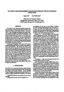
the erroris distribution. The validated to justify its model accuracy. First of all, we thethe n-fold crossmodel validation method toseveral examinetimes the accuracy of the for individual TCs. Toadopted begin with, 16,126 images are divided into mutually exclusive 325 individual TC groups. Then, the validation are cross validation method to examine the accuracy of the model for individual TCs. To begin with, The model is validated several times to justify its out accuracy. First of all, weusing adopted the n-fold performed 325are times. For each we leave one case and train the the remaining the 16,126 images divided intotime, mutually exclusive 325 individual TCmodel groups. Then, the validation cross validation method to that, examine the accuracy ofisthe model using for individual TCs. To begin with, the 324 cases iteratively. After the trained model validated the one which was not included are performed 325 times. For each time, we leave one case out and train the model using the remaining 16,126 images are divided into mutually exclusive 325 individual TC groups. Then, the validation are into training the model. Note although this produced 325 models, the differences among these 325 324 cases iteratively. AfterFor that, the trained model iscase validated using themodel one which wasremaining not included performed 325 times. each time, we leave one out and train the using the models are quite small (not shown here for avoiding redundancy) and are similar with the one into training the model.After Note this produced 325 using models, thewhich differences among these 324 casesabove. iteratively. that,although the process, trained model is validated the one included showed In each validation the distribution of the mean absolute was errornot (MAE), the 325 models are the quite small (notalthough shown error hereproduced for avoiding redundancy) and are similar into training themean model. Note this 325 models, the differences among 325 RMSE and absolute relative (MARE) are calculated(Figure 4). Figure 4a these plotswith the the one showed above. In each validation process, the distribution of the mean absolute error (MAE), models are quite small (not shown here for avoiding redundancy) and are similar with the one distribution of the errors which is obtained by an accumulating procedure of the 16,126 images. It can showed above. In each validation process, the distribution of the mean absolute error (MAE), the the RMSE and the mean absolute relative error (MARE) are calculated (Figure 4). Figure 4a plots be seen that 50%, 75% and 90% of the model estimated intensities are with the MAE less than 7, 13, the RMSE the mean which absolute error (MARE) areRMSE calculated(Figure Figure 4aimages. plotscases theIt can distribution of the errors is relative obtained by accumulating procedure of4).TCs. the 16,126 and 20 and knot, respectively. Figure 4b shows thean average of for individual For the 325 distribution of the errors which is obtained by an accumulating procedure of the 16,126 images. It can in the dependent test, well over their intensities estimated are withwith a mean 127, 13, be seen that 50%, 75% and 90% of75% the of model estimatedare intensities theRMSE MAEless lessthan than be seen that only 50%, 18 75% and 90%15ofknot. the modelaveraged estimated intensities areknot withfor thethe MAE less than 7, 13, knot, while TCs over is 18.52 overall and 20 knot, respectively. Figure 4b showsThe the averageRMSE of RMSE for individual TCs. For325 thecases. 325 cases and 20 4c,d knot,plots respectively. Figure 4b shows the average of(defined RMSE for TCs. For the 325 cases thewell averaged averaged bias asindividual the average between in theFigure dependent test, over MARE 75% ofand their intensities are estimated with adifferences mean RMSE less than in the dependent test, well over 75% of their intensities are estimated with a mean RMSE less than 12 the estimated intensity and the best-track intensity) for the 325 cases, respectively. The mean MARE 12 knot, while only 18 TCs over 15 knot. The averaged RMSE is 18.52 knot for the overall 325 cases. knot, while only 18 TCs over 15 knot. The averaged RMSE is 18.52 knot for the overall 325 cases. is 19.91% and the mean bias is −0.56 knot (while the mean absolute bias is 4.47 knot). Figure 4c,d 4c,d plotsplots the the averaged MARE bias(defined (definedasas the average differences between Figure averaged MAREand andaveraged averaged bias the average differences between 60andand 25 the estimated intensity thethe best-track intensity) for the 325 cases, respectively. The mean MARE is the estimated intensity best-track intensity) for the 325 cases, respectively. The mean MARE (b) Mean: 8.52 (a) 20 19.91% and theand mean bias is ´0.56 knot (while the mean absolute bias 4.47 knot). is 19.91% the mean bias is −0.56 knot (while the mean absolute bias is 4.47 knot). 40 15

10 25 (a) 5 Mean: 8.52 20 0 90 100 150 50 100

(b)

25 50 75 150 200 250 300 Percent (%) Typhoon No 10 20 Mean: 19.91 (c) Mean: 0.56 (d) 10 13 40 5 7 30 0 00 0 25 50 75 90 100 0 50 100 150 200 250 300 Percent (%) Typhoon No 20 (c) -10 Mean: 0.56 Mean: 19.91 (d) 10 10 40 3000 50 100 150 200 250 300 50 100 150 200 250 300 00 Typhoon No Typhoon No 20 -10 N-fold10cross validation of the model using the 325 cases in the northwestern pacific

Figure 4. Ocean during the time 0period 2007.250 (a) The of the errors. (b) 0 50 from 100 1996 150 to 200 300 cumulative 0 50 distribution 100 150 200 250 absolute 300 Typhoon No Typhoon No The root mean square error for each left out case. (c) The absolute relative error for each left out case. Figure 4. N-fold cross validation themodel modelusing using the the 325 northwestern pacific Ocean (d)4.The bias for each left out case. Figure N-fold cross validation ofofthe 325cases casesininthe the northwestern pacific Ocean during the time period from 1996 to 2007. (a) The cumulative distribution of the absolute errors. (b) during the time period from 1996 to 2007. (a) The cumulative distribution of the absolute errors; The root mean square error for each left out case. (c) The absolute relative error for each left out case. (b) The root mean square error for each left out case; (c) The absolute relative error for each left out (d) The bias for each left out case.

case; (d) The bias for each left out case.

Atmosphere 2016, 7, 40 Atmosphere 2016, 7, 40

9 of 17 9 of 16

In order order to toexamine examine whether whether the the performance performance of of the the model model relies relies on on the the category category of of the the TC TC In intensity, the 16,126 images are divided into every 5 knot bins. Figure 5a shows the counts of TCs in intensity, the 16,126 images are divided into every 5 knot bins. Figure 5a shows the counts of TCs in eachintensity intensitybins binsin inthe thedependent dependenttests. tests.Figure Figure5b 5bshows showsthat thatthe themean meanRMSE RMSEgenerally generallyincreases increases each with intensity but for intense typhoons (≥130 Knot). However, from Figure 5c, the MARE, canbe be with intensity but for intense typhoons (ě130 Knot). However, from Figure 5c, the MARE, ititcan found that the absolute relative error is not significant (≤15%) for TCs stronger than 60 knot, which found that the absolute relative error is not significant (ď15%) for TCs stronger than 60 knot, which meansthat thatalthough althoughmore moreerrors errorscould couldbe beexpected expectedfor forintense intensetyphoons, typhoons,the therelative relativeerror errorisisquite quite means small. From Figure 5d, the model generates noticeable (absolute bias > 10 Knot) overestimation in small. From Figure 5d, the model generates noticeable (absolute bias > 10 Knot) overestimation in casesof ofweak weaksystems systems(ď25 (≤25 knot) knot) and and underestimation underestimation in in cases cases of of intense intense (ě150 (≥150 knot). cases knot).

Count

RMSE (knot)

2000 1000

MARE (%)

50

45

70 95 Intensity Bin (knot) Mean: 15.45 %

120

145 (c)

40 30 20 10 20

45

70 95 120 Intensity Bin (knot)

145

(b)

Mean: 11.81 Knot

15 10 5 20 10

BIAS (knot)

0 20

20

(a)

45

70 95 120 Intensity Bin (knot) Mean: -4.17 Knot

145 (d)

0 -10 20

45

70 95 120 Intensity Bin (knot)

145

Figure Figure5.5. Results Results of of the the dependent dependent tests testsby byintensities intensitiesbins. bins. (a) (a) The The frequency frequency distribution distribution of ofthe the cyclones by intensity in the dependent tests; The average: (b) root mean square error; (c) absolute cyclones by intensity in the dependent tests; The average: (b) root mean square error; (c) absolute relative and (d) (d) biasbias for each intensity bin. bin. relativeerror; error; and for each intensity

Tofacilitate facilitatefurther furtheranalysis, analysis,the the16,126 16,126images imagesare arethen thendivided dividedinto intoseven sevengroupsaccording groupsaccordingto to To Saffir–SimpsonScale. Scale.The TheRMSE RMSEand andMARE MAREare arecalculated calculated for for each each group. group. Table Table 44 shows shows the the results. results. Saffir–Simpson Ingeneral, general,the theerror errorincreases increaseswith with intensity, with RMSE 10.52, 12.94, 15.68, 17.49 18.93 In intensity, with thethe RMSE 10.52, 12.94, 15.68, 17.49 andand 18.93 knotknot for for category 1–5 typhoons, respectively. However, from the MARE (last column in Table 4), it can be category 1–5 typhoons, respectively. However, from the MARE (last column in Table 4), it can be found found the performs model performs for tropical depressions and storms see Figures and 5) that thethat model well butwell for but tropical depressions and storms (also see(also Figures 3 and 5)3 which which has the highest proportion of samples (63.66%). The MARE between the regressed and the has the highest proportion of samples (63.66%). The MARE between the regressed and the interpolated interpolated best-track intensities for tropical depressions is as although high as 30.35% although the RMSE best-track intensities for tropical depressions is as high as 30.35% the RMSE is relatively smallis relatively (7.77 Figures and 5d, Table all is suggest this is due to(96.74%) an overestimate (7.77 knot).small Figures 3aknot). and 5d, Table 43aall suggest that 4this due tothat an overestimate for this (96.74%) while for this category, for the category model tends As to aproduce category, for category 1–5while typhoons, model 1–5 tendstyphoons, to producethe underestimations. whole, underestimations. As a whole, all the images, 57.76% (9314) are overestimated while 42.24% for all the 16,126 images, 57.76%for (9314) are16,126 overestimated while 42.24% (6812) are underestimated. The (6812) RMSE are underestimated. Theseeoverall is 12.69 (also see and Figure 3a). overall is 12.69 knot (also Table 4RMSE and Figure 3a). knot Meanwhile, theTable overall4 MARE is 19.78% Meanwhile, the overall MARE is 19.78% which is resulted primarily from tropical storms and which is resulted primarily from tropical storms and depressions, when they are removed from the depressions, when are MARE removed from the tests, the overall MARE deceases to 12.55% dependent tests, thethey overall deceases to dependent 12.55% for all category 1–5 typhoons. for all category 1–5 typhoons. Table 4. Dependent tests of the model by dividing the cyclones into seven groups according to Saffir–Simpson Scale. The number and ratio of underestimated or overestimated images are listed in the table. Bins Tropical Depression Tropical Storm C1 (Typhoon) C2 (Moderate Typhoon)

No. of Samples (%) 4752 (29.47) 5513 (34.19) 2444 (15.16) 1242 (7.70)

No. of Overestimated (%) 4597(96.74) 3575 (64.85) 766 (31.34) 397 (31.96)

No. of Underestimated (%) 155 (3.26) 1938 (35.15) 1678 (68.66) 845 (68.04)

RMSE (Knot) 7.77 9.95 10.52 12.94

MARE (%) 30.35 18.46 12.71 14.79


10 of 17

Table 4. Dependent tests of the model by dividing the cyclones into seven groups according to Saffir–Simpson Scale. The number and ratio of underestimated or overestimated images are listed in the table. No. of Samples (%)

Bins

No. of Overestimated (%)

Tropical Depression 4752 (29.47) Tropical Storm 5513 (34.19) C1 (Typhoon) 2444 (15.16) C2 (Moderate Typhoon) 1242 (7.70) C3 (Severe Typhoon) 910 (5.64) Atmosphere 2016, 7, 40 C4 (Super Typhoon) 1041 (6.46) C5 (Extreme Typhoon) 224 (1.39) C3 (Severe Typhoon) 16,126910 (5.64) Overall (100) C4 (Super Typhoon) 1041 (6.46) C5 (Extreme Typhoon) 224 (1.39) 4.2. Independent Tests Results 16,126 (100) Overall

No. of Underestimated (%)

4597(96.74) 3575 (64.85) 766 (31.34) 397 (31.96) 247 (27.14) 391 (37.56) 107 (47.76) (27.14) 9314247 (57.76) 391 (37.56) 107 (47.76) 9314 (57.76)

RMSE (Knot)

155 (3.26) 1938 (35.15) 1678 (68.66) 845 (68.04) 663 (72.86) 650 (62.44) 117 (52.24) 663 (72.86) 6812 (42.24) 650 (62.44) 117 (52.24) 6812 (42.24)

7.77 9.95 10.52 12.94 15.68 17.49 18.93 15.68 12.69 17.49 18.93 12.69

MARE (%) 30.35 18.46 12.71 14.79 14.26 1011.82 of 16 10.69 14.26 19.78 11.82 10.69 19.78

The developed model is run on 52 cases (see Figure 6 and Table 1 for detail number and percent 4.2. Independent Tests Results of images in each group) from the 2008 to 2009 typhoon season for validation. Of the 52 cases, The developed model is23 run 52 cases storms, (see Figure 6 and 1 for detail number and percent five are tropical depressions, areontropical five are Table typhoons, six are moderate typhoons, of images in each group) from the 2008 to 2009 typhoon season for validation. Of the 52 cases, three are severe typhoons, five are super typhoons, and fvie are extreme typhoons. Because thisfive 52 cases are tropical depressions, 23 are tropical storms, five are typhoons, six are moderate typhoons, three are not included in training the model, the results of the independent tests are indicative of what we are severe typhoons, five are super typhoons, and fvie are extreme typhoons. Because this 52 cases can expect when this model is applied into real-time estimation process. For the aim of comparison are not included in training the model, the results of the independent tests are indicative of what we among groups with approximately same size. The 52 cases are divided into three groups by thresholds can expect when this model is applied into real-time estimation process. For the aim of comparison