Cytometry Part B (Clinical Cytometry) 54B:46 –53 (2003)
Multiple Method Comparison: Statistical Model Using Percentage Similarity Lesley E. Scott,1* Jacky S. Galpin,2 and Deborah K. Glencross 1
Department of Molecular Medicine and Hematology, Faculty of Health Sciences, University of the Witwatersrand, Johannesburg, South Africa 2 Department of Statistics and Actuarial Science, University of the Witwatersrand, Johannesburg, South Africa
Background: Method comparison typically determines how well two methods agree. This is usually performed using the difference plot model, which measures absolute differences between two methods. This is often not applicable to data with wide ranges of absolute values. An alternative model is introduced that simplifies comparisons specifically for multiple methods compared to a gold standard. Methods: The average between a new method and the gold standard is represented as a percentage of the gold standard. This is interpreted as a percentage similarity value and accommodates wide ranges of data. The representation of the percentage similarity values in a histogram format highlights the accuracy and precision of several compared methods to a gold standard. The calculation of a coefficient of variation further defines agreement between methods. Results: Percentage similarity histograms of several new methods can be compared to a gold standard simultaneously, and the comparison easily visualized through use of a single 100% similarity reference line drawn common to all plots. Conclusion: This simple method of comparison would be particularly useful for multiple method comparison and is especially applicable for centers collating for external quality assessment or assurance programs to demonstrate differences in results between laboratories. Cytometry Part B (Clin. Cytometry) 54B: 46 –53, 2003. © 2003 Wiley-Liss, Inc. Key terms: statistical multiple method comparison, Bland-Altman difference plots, percentage similarity, histogram (frequency distribution), accuracy and precision, coefficient of variation
CD4 T-cell enumeration data range from very low (⬍10 cells/l) to very high (⬎3,000 cells/l) cell numbers, which are used for immune monitoring of disease progression of human immunodeficiency virus to acquired immunodeficiency syndrome (1). The introduction of new methods or strategies for cell counting requires statistical evaluation, if the aim is to replace one technique with another. Data from a CD4 T-cell enumeration study was used (2) to introduce and demonstrate the usefulness of a percentage similarity histogram model. This study required evaluation of several CD4 T-cell enumeration assays by flow cytometry to determine the accuracy and precision of a new gating strategy. The difference plot or Bland-Altman plot (3) is well recognized as the method of choice for measuring agreement between two methods. The difference between data pairs (a ⫺ b) is graphically represented on the vertical axis against their average [(a ⫹ b)/2] on the horizontal axis. The absolute observation, and not the average, is often used if method b is the known gold standard, because the gold standard is generally ac-
© 2003 Wiley-Liss, Inc.
cepted as the method with the least error. The mean paired difference (the bias) and the limits of agreement [mean ⫾ 2 standard deviation (S.D.)] are illustrated on the plots. Confidences intervals (usually 95%) for the mean difference and the limits of agreement are calculated to determine the range in which the true values may lie, because a new sample drawn from the same population would yield slightly different descriptives. Ideally two methods compare favorably when the mean paired difference is close to zero (a zero mean difference implies equality), limits of agreement are narrow, and few outliers are present. Bland-Altman analysis is best applied when the range of absolute values is narrow and the absolute differences are small. The analysis is *Correspondence to: Lesley E. Scott, Department of Molecular Medicine, University of the Witwatersrand, 7 York Road Parktown 2193, Johannesburg, Gauteng 2000, South Africa. E-mail:
[email protected] Received 15 October 2002; Accepted 7 January 2003 Published online in Wiley InterScience (www.interscience.wiley.com). DOI: 10.1002/cyto.b.10016
47
STATISTICAL METHOD COMPARISON
FIG. 1. B-A–F-A: Typical Bland-Altman plots of five (new) methods compared with the gold standard (A) demonstrating absolute differences of CD4 T-cell counts. The mean differences and limits of agreement are shown in each plot. Outliers are represented as points on the outer side of the limits of agreement. In most plots, these points indicate values greater than 1,000 cells/l. The Bland-Altman plots of all new methods versus the gold standard show a fan-shape trend over the range. This is emphasized in the plot D-A by the dotted lines. STD, standard deviation. [Color figure can be viewed in the online issue, which is available at www.interscience.wiley. com.]
cumbersome when there is a wide range of absolute values or multiple method comparisons are required. The simpler approach to method comparison is using the percentage similarity between data pairs and not absolute differences. In this report, we demonstrate that the use of the percentage similarity plotted as a histogram, including a normal curve with relevant mean and S.D., to calculate a coefficient of variation (C.V.) that allows for a more meaningful and better visual comparison of methods. The percentage similarity value between each new method and the gold standard is calculated as the average between the new method and the gold standard (the numerator) divided by the gold standard (the denominator) multiplied by 100. Data pairs with the same value will be 100% similar. Data pairs in which the new method is greater than the gold standard will be greater than 100%;
conversely, data pairs in which the new methods is less than the gold standard will be less than 100%. The aim of this report was to demonstrate the usefulness of this new approach compared with the more conventional described difference plot, especially in the context of multiple methods compared with a gold standard. MATERIALS AND METHODS Sample Data One hundred twelve samples were used to evaluate six different flow cytometric CD4 T-cell enumeration methods. Descriptions of these methods, designated A through F, follow. A: Single-platform volumetric method using three tubes (full panel, Ortho Trio): isotype control, CD4/CD8/CD3, and CD16/CD19/CD3.
48
SCOTT ET AL.
B: Dual-platform light scatter lymphocyte gated in one tube: CD8/CD4/CD3 (Crystostat™, Beckman Coulter, Fullerton, CA. The lymphocyte differential is used to calculate the absolute CD4 count. C: Single-platform microsphere using TruCount (BD Biosciences, San Jose, CA) in one tube: CD3/CD4/CD45 (TriTEST™ BD Biosciences). The lymphocytes are gated with CD3 and side scatter parameters. D: Dual-platform PanLeucogated in one tube: CD45 (Beckman Coulter)/CD4 (RFT4). This is a new concept that measures CD4 cells as a percentage of all leukocytes and calculates the absolute CD4 count by using the white cell count from a hematology analyzer. E: Dual-platform bright CD45 lymphocyte gated in one tube: CD45 (Beckman Coulter)/CD4 (RFT4). The lymphocyte differential is used to calculate the absolute CD4 count. F: Single-platform volumetric PanLeucogated in one tube: CD45 (Hle-1)/CD4 (RFT4).
the true trend in this data set, but the bias, the log limits of agreement and the negative log scale, are not easily interpreted back to absolute values as measures of agreement. The Bland-Altman statistics derived from plots shown in Figures 1 and 2 are summarized in Table 1. These statistics suggest that method F and, to a lesser extent, method D are good replacements for the gold standard, method A, when using the small bias, narrow confidence intervals and limits of agreement for the untransformed and transformed data. Method C also has a small bias, but the limits of agreement are much wider, as is the confidence interval of the mean. Multiple method comparison requiring all these statistics is cumbersome.
Method A was considered the gold standard against which all other techniques were compared (2). The CD4 T-cell enumeration absolute cell count observations ranged from 1 to 2,000 cells/l, with most observations being fewer than 500 cells/l.
[({a⫹b}/2)/a]⫻100
Data Pair Comparisons All statistical models were analyzed with SPSS 10 and SAS Enterprise Guide release 1.3. Bland-Altman statistics and the new percentage similarity histogram plots were applied to compare the respective methods to determine the best replacement for the gold standard, method A. RESULTS Bland-Altman Model Bland-Altman plots of the five methods versus the gold standard, method A, are shown in Figure 1. The absolute values of the gold standard, not the average between method A and methods B–F, are represented on the horizontal axes. All 112 data pairs are represented, which made representing all plots on the same y-axis scale cumbersome, but no outliers were removed. The plots demonstrate that most observations below are 500 cells/l. However, most outliers were in the ⬎1,000 cells/l range, and this produced a fan-shape trend over the range in all method comparisons, as outlined by one example (Fig. 1D-A). This fan-shape trend suggested that the difference between data pairs is not relative over the range and may require transformation of the raw data (3). Figure 2 shows the differences between the log-transformed data on the vertical axis and the absolute values of the gold standard on the horizontal axis. The log-transformed Bland-Altman plots show that most outliers were in the absolute ⬍50 cells/l counting range. This observation is compatible with the knowledge that flow cytometric and hematologic instruments show more instrument variability and inaccuracies at very low ranges of cell counting (4). The log-transformation may better represent
Percentage Similarity Model The percentage similarity values from data pairs of each new method compared with the gold standard (method A) were calculated with the formula
where a is the gold standard and b is the new method. Figure 3 shows these percentage similarity values plotted on the vertical axis of a scatterplot versus the absolute values of the gold standard on the horizontal axis in a format similar to the Bland-Altman plots. Each scatterplot shown in Figure 3 illustrates that most data pairs with the least percentage similarity (outliers) are in the absolute range of ⬍50 cells/l. This is confirmed by the log-transformed data in the Bland-Altman plots shown in Figure 2, where most of the methods are least accurate in this low data range. A CD4 T-cell count of 50 cells/l, or 50% less similarity at 25 cells/l, has the same clinical outcome and treatment (5); therefore, the large percentage difference in this data range is not considered clinically relevant. Scatterplots of the percentage values are a good visual representation of the true trend within this data set. The real application and usefulness of the percentage similarity values concerns representing the values in a histogram format. The percentage similarity values are grouped into intervals and plotted on the horizontal axis against the number in each interval, as shown in Figure 4. A useful feature of histograms is that a normal curve (Fig. 4B) can be fitted to those intervals, with a mean and S.D. calculated from the data. The normal curve plotted over the intervals illustrates the spread (S.D.) of these percentage similarity values around the peak (mean). The distance of the peak from the 100% similarity line, or 0% difference reference line, indicates the amount of bias between the two methods. The mean percentage similarity value in the example in Figure 4 is 96%, which shows that the new method has a mean bias of 4% less than the gold standard. The S.D. in this example is 11.2% and is a measure of the spread of the normal curve. Together these parameters are summarized as the difference: mean percentage difference (M.P.D.) ⫾ S.D. For the example shown in Figure 4, this difference is M.P.D. ⫽ 4 ⫾ 11.2%. The mean percentage similarity and
STATISTICAL METHOD COMPARISON
49
FIG. 2. LogB-LogA–LogF-Log A: Bland-Altman plots of log-transformed raw data of all five (new) methods compared with the gold standard (A). The mean differences and limits of agreement are shown in each plot. Outliers are points on the outer side of the limits of agreement. In most plots, these points represent values less than 50 cells/liter. STD, standard method A. [Color figure can be viewed in the online issue, which is available at www. interscience.wiley.com.]
the S.D. also can be used to calculate a C.V. between the two methods. The C.V. is calculated by dividing the S.D. by the mean percentage similarity. In this example, the C.V. is 11.6% (11.2 of 96, expressed as a percentage). This summarizes the mean and the spread into one unit of overall agreement between the two methods. Percentage similarity histograms are visually comparable, especially for multiple method evaluation, because the 100% similarity point is central and common to all plots irrespective of the spread caused by outliers. Normal curves with the highest peak show the greatest accuracy between method pairs. Normal curves with the widest
spread show the least precision between method pairs. Figure 5 shows various visual characteristics of normal curves. These characteristics also can be described with the mode (the value of the variable that occurs most frequently) of the histogram. A mode and a mean percentage similarity that are different illustrate a skewed distribution with a method pair of poor agreement. The histogram shape is a function of the number of intervals. Several histograms can be visually compared when selecting the same number of intervals for each plot (a feature of SPSS). Alternatively (a feature of SAS), the 100% similar (0%
50
SCOTT ET AL.
Table 1 Bland-Altman Statistics Data pair B–A C–A D–A E–A F–A B–A C–A D–A E–A F–A
Bias (mean difference)
Confidence interval of the mean
Limits of agreement
Untransformed data from Figure 1 ⫺46.18 ⫺76 to ⫺16 275, ⫺368 ⫺16.23 ⫺32 to ⫺0.2 155, ⫺188 ⫺16.88 ⫺23 to ⫺11 49, ⫺83 ⫺25.68 ⫺33 to ⫺19 50, ⫺102 ⫺8.16 ⫺12 to ⫺5 30, ⫺46 Log-transformed data from Figure 2 ⫺0.037 ⫺0.059 to ⫺0.014 0.203, ⫺0.277 0.0039 ⫺0.029 to 0.037 0.36, ⫺0.35 ⫺0.025 ⫺0.036 to ⫺0.013 0.096, ⫺0.15 ⫺0.042 ⫺0.059 to ⫺0.026 0.14, ⫺0.22 ⫺0.028 ⫺0.041 to ⫺0.014 0.12, ⫺0.18
difference) reference line together with the 50% lower limit and 150% upper limit lines can be included for direct visual comparison, as in Figure 6. The mode for each histogram is 100, illustrating no gross irregularities in any of the new methods. Histograms F and D visually compare well with the gold standard, followed by method E, which has a larger spread. Only methods B and C show intervals past the limit lines, indicating a large spread around the mean and lack of precision. Further examination of the method C histogram shows only a few gross outliers (also noted in the scatterplot in Fig. 3), which may indicate unfamiliarity with the technique (according to method B in the key Fig. 5). Although visual inspection of the histograms indicates good and poor methods as compared with the gold standard, Table 2 summarizes these differences more clearly.
FIG. 3. B–F: Scatterplots of data pair percentage similarity (vertical axis) for all (new) methods versus the absolute values of the gold standard (horizontal axis). All 112 data pairs are included in all plots. STD, standard method A. [Color figure can be viewed in the online issue, which is available at www.interscience.wiley.com.]
STATISTICAL METHOD COMPARISON
FIG. 4. Example of a percentage similarity scatterplot (A) and histogram (B) comparing a new method with the gold standard. The scatterplot is placed on end to illustrate the transition into the histogram. Percentage similarity data from the scatterplot are grouped into 25 intervals and plotted (horizontal axis) against the count (vertical axis). The normal curve is plotted over the histogram with a line to the 100% similarity (or 0% difference) point. [Color figure can be viewed in the online issue, which is available at www.interscience.wiley.com.]
51
The R2 value indicates how well the linear regression model fits the data. Correlation and linear regression are not suited to measure agreement between methods because both are strongly influenced by outliers and observations with large values. The high values from broad data ranges will improve r and R2 and the slope of the line. This is often the case with cell enumeration observations with values that range from fewer than 10 cells/l to more than 1,000 cells/l in the same data set. The Bland-Altman or difference plot (3) is the method of choice for determining agreement between two methods. The mean difference indicates bias between two methods, and agreement is based on the significance of the spread of the limits of agreement. Data often encountered with cell counting techniques that span broad ranges require transformation when the difference is not relative over the range (3). Transformations are seldom applied because significance of transformed differences is not easily interpreted. Several alternative models for method comparison specifically designed for graphic interpretation have been introduced in the literature. A modified Bland-Altman plot (6) calculates the difference between two results and expresses that difference as a percentage of the mean of the two measurements. This is plotted against their mean in a scatterplot. The folded empirical cumulative distribution, or mountain plot (7), ranks the differences (or percentage differences), computes a percentile for each difference, and plots the percentile against the differences.
All new methods except method C produced results on average lower than the gold standard (as shown by the mean bias). Methods D, F, and B appear to have the greatest accuracy according to their M.P.D.s (distance of their mean from the 100% reference line). Methods F and D appear to have the best precision (corresponding to the lowest S.D.). Overall agreement with the gold standard (method A) is met best by methods F and D, because their C.V.s are the lowest, which reflects accuracy and precision. These plots are especially useful for researchers who are not familiar with or who have difficulty conceptualizing Bland-Altman difference plots and logarithmic transformations. DISCUSSION The introduction of new methods or techniques in any field of study requires statistical evaluation with the aim of replacing one technique with another. A typical approach adopted by many investigators for evaluating method comparison includes the correlation coefficient (r), linear regression (using R2 and the slope of the line), and difference plots (3). However, correlation is intended for two different variables to identify a nonlinear trend, and the correlation coefficient (r) measures the strength of the linear relation between the two variables. Linear regression quantitates this linear relation by calculating the coefficients of the equation (y ⫽ a ⫹ bx) and is best applied for predicting one variable from another by using this equation of the line.
FIG. 5. Examples of normal curves showing their spread around the 100% similarity reference line. Accuracy reflects how good a new method is, and precision reflects the technique of the operator (how well the method is performed).
52
SCOTT ET AL.
FIG. 6. The five percentage similarity histograms of each new method (B, C, E, F) versus the standard (A). The upper (150%) and lower (50%) limits and the 100% similarity reference line are indicated in each plot. The horizontal axis represents the percentage similarity values in intervals, and the vertical axis represents the number (percentage of the total number) of percentage similarity values in each interval. The legend for each plot lists the mean percentage similarity (mu) and the percentage of standard deviation (sigma; n ⫽ 112). [Color figure can be viewed in the online issue, which is available at www.interscience.wiley.com.]
Although these alternative approaches were introduced to deal with absolute data values with broad ranges, they have not attained widespread application as the simpler
Bland-Altman approach. However, the Bland-Altman approach is often ill applied and is cumbersome for multiple method comparisons.
Table 2 Summary of the Percentage Similarity Histogram and Normal Curve Statistics Method pair with Aa B C D E F
Mean similarity ()
S.D. similarity ()
97.5% 106.9% 97.7% 96.3% 97.5%
11.77% 44.63% 6.8% 9.19% 6.31%
M.P.D. ⫾ S.D. 2.5 6.9 2.3 3.7 2.5
⫾ ⫾ ⫾ ⫾ ⫾
11.77% 44.63% 6.8% 9.19% 6.31%
C.V. 12.1% 41.7% 6.96% 9.54% 6.47%
a The gold standard is used as coefficient a in the formula (n ⫽ 112). C.V., coefficient of variation; M.P.D., mean percentage difference; S.D., standard deviation.
53
STATISTICAL METHOD COMPARISON
The relation between data pairs expressed as a percentage value rather than an an absolute difference has certain advantages. The percentage similarity values can be applied to any range of data and, in a sense, standardizes data over all ranges. The M.P.D. ⫾ S.D. addresses the issue of accuracy and precision between a new and existing (gold standard) technology. Overall, one unit, the C.V., interprets agreement, which is comparable between multiple methods and the same gold standard. Not representing the Bland-Altman plots on the same y-axis scales for visual comparison of methods can be criticized, but it is cumbersome and often not meaningful without excluding outliers. Researchers require a simple and interpretable model that does not rely too heavily on a statistical understanding. The percentage similarity histogram has no negative scale, and the 100% similarity (0% difference) point is central and common to all percentage similarity plots. In the example of the five flow cytometric methods of CD4 testing for monitoring of acquired immunodeficiency syndrome, the choice of a suitable replacement for the gold standard is a decision that affects the accuracy of the test and its availability and affordability to the individual patient. An incorrect choice seriously affects health care budgets and laboratory management decisions to replace existing technology (2). The Bland-Altman model and the percentage similarity model determined methods F (single-platform PanLeucogated) and D (dual-platform PanLeucogated) as suitable replacements for the gold standard (single-platform volumetric; Ortho Trio). The percentage similarity model also explains the poor agreement of methods E, B, and C by describing their lack of accuracy and/or precision with the gold standard. The
percentage similarity model is not intended to replace existing models, but is complementary and designed especially for comparing multiple methods with a gold standard. The C.V. generated by the percentage similarity model allows multiple methods to be compared based on overall agreement with a gold standard. This is advantageous for investigators to compare their methods worldwide, which is especially important for participation in external quality assurance programs. ACKNOWLEDGMENTS We thank Dr. Ilesh Jani and Prof. George Janossy, HIV Immunology, Department of Immunology and Molecular Pathology, Royal Free and University College Medical School, London, United Kingdom, for their valuable comments and for providing some of the raw data. LITERATURE CITED 1. Stein DS, Krovick JA, Vermund SH. CD4⫹ lymphocyte cell enumeration for prediction of clinical course of HIV disease: a review. J Infect Dis 1992;165:352. 2. Glencross DK, Scott LE, Jani IV, Barnett D, Janossy G. CD45-assisted PanLeucogating for accurate, cost-effective dual platform CD4⫹ T-cell enumeration. Clin Cytometry 2002;50:69 –77. 3. Bland JM, Altman DG. Statistical methods for assessing agreement between two methods of clinical measurement. Lancet 1986;8:307– 310. 4. Simson E, Groner W. Variability in absolute lymphocyte counts obtained by automated cell counters. Cytometry 1995;22:26 –34. 5. Hoover DR, Graham NMH, Chen B, et al. Effects of CD4⫹ cell count measurement variability on staging HIV-1 infection. J Acquir Immune Defic Syndr 1992;5:794. 6. Pollock MA, Jefferson SG, Kane JW, Lomax K, MacKinnon G, Winnard CB. Method comparison—a different approach. Ann Clin Biochem 1992;29:556 –560. 7. Krouwer JS, Monti KL. A simple, graphical method to evaluate laboratory assays. Eur J Clin Chem Clin Biochem 1995;33:525–527.