this technique for a range of nonlinear control problems. ... University of Belfast, Ashby Building, Stranmillis Road, Belfast BT9 5AH, N. Ireland, UK. E-mail: g.
Transactions of the Institute of Measurement and Control http://tim.sagepub.com
Multiple model nonlinear control of synchronous generators M. D. Brown, D. Flynn and G. W. Irwin Transactions of the Institute of Measurement and Control 2002; 24; 215 DOI: 10.1191/0142331202tm057oa The online version of this article can be found at: http://tim.sagepub.com/cgi/content/abstract/24/3/215
Published by: http://www.sagepublications.com
On behalf of:
The Institute of Measurement and Control
Additional services and information for Transactions of the Institute of Measurement and Control can be found at: Email Alerts: http://tim.sagepub.com/cgi/alerts Subscriptions: http://tim.sagepub.com/subscriptions Reprints: http://www.sagepub.com/journalsReprints.nav Permissions: http://www.sagepub.com/journalsPermissions.nav
Downloaded from http://tim.sagepub.com at PENNSYLVANIA STATE UNIV on April 17, 2008 © 2002 SAGE Publications. All rights reserved. Not for commercial use or unauthorized distribution.
Transactions of the Institute of Measurement and Control 24,3 (2002) pp. 215–230
Multiple model nonlinear control of synchronous generators M.D. Brown1 , D. Flynn2 and G.W. Irwin 2 1
WS Atkins Consultants Ltd, Bristol BS32 45Y, UK School of Electrical and Electronic Engineering, The Queen’s University of Belfast, Ashby Building, Stranmillis Road, Belfast BT9 5AH, UK 2
Research has shown that conventional adaptive control and more sophisticated nonlinear approaches can suffer from a lack of robustness and transparency. In this paper, a multiple model technique is proposed that effectively incorporates established linear control methods within an inherently nonlinear framework. The resulting local model network (LMN) was found to describe the nonlinear dynamics of a laboratory turbogenerator excitation loop over its useful operating range. A simple nonlinear generalized minimum variance (GMV) controller was then designed for this system and compared with an adaptive GMV controller. The excellent control performance and transparent nature of the LMN illustrates the potential for this technique for a range of nonlinear control problems. Key words: local model networks; multiple controllers; nonlinear control; synchronous generators
1.
Introduction
The ever-increasing demand for efciency and improved performance has prompted a move towards more complex control strategies for industrial processes. Nonlinear behaviour, unknown process parameters and variable plant transfer functions due to changing plant throughput all contribute to the problems faced by practical control engineers. Although conventional control schemes, such as PID, are widely used, their performance is often poor, and, in the case of plants Address for correspondence: G.W. Irwin, School of Electrical & Electronic Engineering, The Queen’s University of Belfast, Ashby Building, Stranmillis Road, Belfast BT9 5AH, N. Ireland, UK. E-mail: g.irwinKee.qub.ac.uk
Ó 2002 The Institute of Measurement and Control 10.1191/0142331202tm057oa Downloaded from http://tim.sagepub.com at PENNSYLVANIA STATE UNIV on April 17, 2008 © 2002 SAGE Publications. All rights reserved. Not for commercial use or unauthorized distribution.
216
Multiple model nonlinear control of synchronous generators
with many control loops, tuning can prove to be a costly and time-consuming business. Research studies have suggested that self-tuning and adaptive control can offer advantages over conventional control implementations (Kanniah et al., 1984; Malik et al., 1992). The adaptive nature of these schemes can take into account the nonlinearities of generation equipment, for example, and automatically compensate for problems arising from plant ageing. Indeed, power system control manufacturers are beginning to apply self-tuning systems commercially (Hingston et al., 1989; Zachariah et al., 1990). However, the main difculty with adaptive control strategies lies in the robustness of the parameter estimation stage. Due to the nonlinear nature of power systems, the derived linear models are only valid around a particular operating point. Sudden changes in operating conditions violate the preconditions for linear identication and this, in turn, leads to problems within the estimator. Nonlinear control using neural networks can overcome some of the difculties faced by linear controllers, and recent research has shown that these techniques can be applied to generator excitation control (Flynn et al., 1997; Ramakrishna and Malik, 2000). However, even this approach has some fundamental limitations. Firstly, the nontransparent, black-box nature of neural networks makes it difcult to interpret their nal structure in terms of the physical characteristics of the process under consideration. Secondly, neural network modelling fails to exploit signicant theoretical results available in the conventional modelling and control domain, making it difcult to analyse their behaviour and investigate stability. The methodology adopted in this paper proposes that a global model of the generator excitation loop dynamics can be constructed from a set of locally valid submodels. The outputs of each submodel are passed through a local processing function that effectively acts to generate a window of validity for the model in question, and the resultant localized outputs are then combined as a weighted sum at the model output node. This local model network (LMN) approach potentially allows conventional modelling and control techniques to be utilized within a nonlinear framework, while offering transparency of operation and the ability to readily incorporate a priori knowledge. Building on simulation studies (Brown and Irwin, 1999), this paper reports on the application of LMNs to the identication of a laboratory microalternator excitation loop. Data was gathered across the operating regions of the generator to form a model of the global system dynamics. The resulting model was then used to form a local model controller for the laboratory microalternator system. 2.
LMNs
An LMN (Murray-Smith and Johansen, 1997) can be thought of as a generalization of a radial basis function neural network and is similar in form to a Takagi– Sugeno fuzzy inference system. The output, yˆ , of the LMN is given by: yˆ = F(c, w) where Downloaded from http://tim.sagepub.com at PENNSYLVANIA STATE UNIV on April 17, 2008 © 2002 SAGE Publications. All rights reserved. Not for commercial use or unauthorized distribution.
(1)
Brown et al. 217
O M
F(c, w) =
fi(c) r i(w)
i=1
In this paper, the M local models fi(c) are linear (but in general can be nonlinear) functions of the measurement vector c, and are multiplied by a basis or interpolation function r i(w) that is a function of the current operating region vector, w. This operating region does not necessarily need to be generated by the full model input vector, c, but can be generated by a subset of the measurement data available. In an LMN, the basis functions r i (w) are commonly chosen to be normalized Gaussian functions: r
i
(w) =
exp(-i w - cii 2 /2s
O M
2 i
exp(-i w - cii 2 /2s
) 2 i
(2) )
i=1
where ci and si dene the centre and width of each multidimensional Gaussian function. r i(w) can be interpreted as a model validity function, that gives a value approaching 1 in regions of w where the local fi(·) are such that F(·,·) is a good approximation to yˆ , and a value close to zero when the local fi(·) are such that F(·,·) is not a good approximation to yˆ . Thus, a model that is locally valid in one operating region (i.e., r i(w) < 1) is gradually replaced by a more suitable model as the operating point changes. If nonlinear local models were used, this would preclude the exploitation of established linear techniques at the control design stage. It is customary, therefore, to use linear local models such as ARX, ARMAX or state-space. If, for example, the local models are of the linear ARX form where r and s are the orders of the plant output, y(k), and input, u(k) respectively, at time k, then the LMN represents the nonlinear ARX (NARX) model: yˆ(k + 1) = B0 u(k) + B1 u(k - 1) + ¼ + Bsu(k - s) + A1 y(k) + A2 y(k - 1) + ¼ + Ar+ 1 y(k - r)
(3)
with the parameters Ai and Bi determined at each operating point, w(k), as follows:
O M
Ai =
j=1
O M
r jw(k)aij, Bi =
r jw(k)bij
(4)
j=1
where bij and aij are the parameters of the local linear ARX models. Note that the parameters Ai and Bi are not simply time-varying quantities, but depend on the operating point, which can be static in nature (Brown et al., 1997). Section 3 details the nature of the nonlinearity for this application. This multiple model approach is naturally best suited to systems whose dynamic characteristics undergo signicant variations as the plant operating point changes. This is indeed the case in the power generation industry, where different dynamic behaviour exists as the plant load prole uctuates. The application of LMNs for plant identication is difcult, however. Any strategy has to take into account the complexity of the target mapping, the representational ability of the local models associated with the interpolation functions, the Downloaded from http://tim.sagepub.com at PENNSYLVANIA STATE UNIV on April 17, 2008 © 2002 SAGE Publications. All rights reserved. Not for commercial use or unauthorized distribution.
218
Multiple model nonlinear control of synchronous generators
selection of measured states that describe the system operating behaviour and the availability of the data. A priori plant knowledge and engineering judgement can be used at this stage. Also, having selected the LMN structure, the next step is to nd the optimal values of the parameters. The method adopted in this paper follows the hybrid optimization strategy proposed in Brown et al. (1997). Here, a least-squares cost function is minimized using nonlinear optimization for the centres and widths (ci and si) of the interpolation functions, followed by linear optimization of the local linear models (bij and aij) at each iteration of the process. 3.
Plant modelling
This section rst outlines the laboratory micromachine system used to obtain the experimental results in this study. The structure of the individual local models, i.e., the model order and the required input and output variables, is then chosen. Prior plant knowledge leads on in the next subsection to the denition of the structure of the LMN, i.e., the number and initial position of the interpolation functions, and the operating point vector. Finally, the optimization process is described and typical plant test results are presented. 3.1
Micromachine system
The laboratory microalternator system consists of a specially designed synchronous generator, with an associated turbine simulator, tied to the laboratory busbar through a delta-star transformer and articial transmission lines (Brown et al., 1995), as shown in Figure 1. The synchronous generator is a 3-kVA, 220-V, 50-Hz, 1500-rpm, four-pole microalternator, whose parameters have been scaled to represent those of a full-size generator. The generator is driven by a separately excited d.c. motor, whose armature current is controlled by the analogue turbine simulation. A three-stage turbine with reheater and fast governor is emulated, with the weighted sum of signals from each stage being proportional to the turbine mechanical power. The micromachine system constitutes a two-rotating mass system, whereas a full-scale system will have up to six or more rotating masses. It is unrealistic, therefore, to expect results comparable to a full-scale generating unit.
Figure 1
Laboratory microalternator system
Downloaded from http://tim.sagepub.com at PENNSYLVANIA STATE UNIV on April 17, 2008 © 2002 SAGE Publications. All rights reserved. Not for commercial use or unauthorized distribution.
Brown et al. 219
However, the micromachine can provide a means of verifying simulations as well as permitting control systems to be tested under real-time conditions with effects such as nonideal transducer characteristics, computational delays, saturation and variations in busbar frequency and voltage. 3.2
Local model structure selection
An automatic voltage regulator (AVR) for the system is derived using a linear single input–single output (SISO) ARX model of the generator–exciter system as: A(z-1 )y(k) = B(z-1 )u(k - 1) + j (k)
(5)
where y(k) is the system output (terminal voltage, Vt), u(k) is the system input, (exciter voltage, Vr), j (k) is a zero mean white noise sequence, at sample time k, and z is the shift operator dened by: znx(k) = x(k + n) Here the polynomials A(z-1 ) and B(z-1 ) are dened as: A(z-1 ) = 1 + a1 z-1 + a2 z-2 + ¼ + ana z-na B(z-1 ) = b0 + b1 z-1 + b2 z-2 + ¼ + bnbz-nb
(6)
where na, nb . 0 A simulation of a single-machine innite-busbar system, with associated stepup transformer and double transmission line, was used in initial identication experiments (Hogg, 1981). The simulation also comprises a boiler/turbine system, which provides mechanical input torque to drive the rotor of the synchronous generator. This system is described using the d-q representation by a set of nonlinear rst-order differential equations (Hogg, 1981). These experiments were veried in practice on the micromachine, and results suggested that second-order ARX models for the AVR, i.e., na = 2, nb = 1, were sufcient to capture the main dynamics. 3.3
LMN representation
In an innite busbar system, the operating point of the alternator is dened in terms of the real power output, Pt, and the reactive power output, Qt, i.e., linear models of the plant are formed in the steady-state for small perturbations about different values of Pt, Qt. For the LMN, therefore, the operating point, w (k), is the vector [Pt (k) Qt (k)]. In order to quantify the nonlinearities present in the turbogenerator system, a series of open-loop step tests was performed in simulation over an extended operating region of the plant. Figures 2 and 3 show both the response time (time to reach approximately 63% of the nal value) and the gain of the plant as both Pt and Qt are varied. All quantities are shown in per unit (p.u.) values and the vertical scales are logarithmic. It is clear that the system is indeed nonlinear, with Downloaded from http://tim.sagepub.com at PENNSYLVANIA STATE UNIV on April 17, 2008 © 2002 SAGE Publications. All rights reserved. Not for commercial use or unauthorized distribution.
220
Multiple model nonlinear control of synchronous generators
Figure 2
Operating point vs response time
Figure 3
Operating point vs gain
Downloaded from http://tim.sagepub.com at PENNSYLVANIA STATE UNIV on April 17, 2008 © 2002 SAGE Publications. All rights reserved. Not for commercial use or unauthorized distribution.
Brown et al. 221
the nonlinearity more pronounced in the leading power factor region where Qt , 0. Note that the plant is open-loop unstable when both Pt is high and Qt is sufciently negative (Weedy, 1984). A preliminary guess for M, the number of local models, was found by inspection of the response time and gain surfaces shown in Figures 2 and 3. Initially, seven local models were used to represent these nonlinear variations, with the majority being placed in the leading power factor region where the rate of change of the nonlinearity is greatest. Subsequent optimization using simulation and plant data proved that a sufciently accurate and parsimonious representation was achieved using only ve local models. In this instance, plant a priori information was usefully employed to aid in the model structure selection. In cases where such information is not available, other methods, e.g., fuzzy clustering (Yoshinari et al., 1993), can be applied. 3.4
Plant test results
The lower limit of around 1.6 s on the simulated plant response time suggests a suitable sample period for steady-state models in the region of 300 ms. Transient controller performance, however, demands a sample period of at least 20 ms to enable boost/buck excitation behaviour post-fault. This requirement not only increases the number of training data vectors required, but could also render the linear optimization badly posed due to over-sampling effects. However, since the operating point does not change signicantly in the steady-state, it was possible to train a LMN using data with a sample period of 300 ms. The interpolation region parameters were then xed, and the local linear models updated using a linear optimization method with the smaller sample period of 20 ms. This not only reduces the data requirements, but also expedites the optimization process. With this in mind, training data were generated on the micromachine with a 20-ms sample period by driving the plant across different regions of the operating space and superimposing small pseudo-random binary sequences (PRBS) on the exciter input. This type of perturbation would be allowable on the real plant, and be largely undetectable, when it moves from one operating point to another during scheduled load-following or two-shifting operations. The data were subsequently decimated, and the LMN trained to form a predictive model with a sample period of 300 ms. The optimized interpolation regions are shown in Figure 4 (a–e). Figures 5 and 6 show operating point variation and some sample results of the actual and predicted terminal voltage about a nominal operating point of Pt = 0.7 p.u. and Qt = 0.1 p.u., respectively. Figure 6(b) shows a zoomed version of a small section of Figure 6, while Figure 6(c) shows the difference between the actual and predicted voltage over the full time period. Here, the LMN is operating in parallel mode with a sample period of 20 ms, i.e., A(z-1 )yˆ(k) = B(z-1 )u(k - 1)
(7)
where yˆ (k) is the system estimated output and u(k) is the system input, at sample time k. Downloaded from http://tim.sagepub.com at PENNSYLVANIA STATE UNIV on April 17, 2008 © 2002 SAGE Publications. All rights reserved. Not for commercial use or unauthorized distribution.
222
Multiple model nonlinear control of synchronous generators
Figure 4
(a–e): LMN interpolation regions
It can be seen that the LMN can predict the plant behaviour well into the future (over 26 000 steps ahead for the test sets shown), despite the fact that the plant operating point, and hence the underlying dynamics, change signicantly during the period of the test. This is evident from Figures 2 and 3, which reveal that the variation in real and reactive power coincides with large changes in the gain and response time of the plant. 4. 4.1
LMN control Control law design
Since the LMN consists of second-order linear models, it is quite straightforward to design appropriate linear controllers. These controllers are interpolated to form Downloaded from http://tim.sagepub.com at PENNSYLVANIA STATE UNIV on April 17, 2008 © 2002 SAGE Publications. All rights reserved. Not for commercial use or unauthorized distribution.
Brown et al. 223
Figure 5
Operating point variation
a composite control output, in a similar manner to the actual model output. In this way, the designer has the freedom to tailor each local controller to the individual local model so as to produce uniform control performance across the operating range. Thus, it is possible to exploit conventional linear control theory within a nonlinear control framework. The method chosen for this study was the standard generalized minimum variance (GMV) algorithm (Wellstead and Zarrop, 1991), since some of the linear models derived in the optimization process are both unstable and nonminimum phase. Due to the transparent nature of the local model plant description, however, any suitable linear design method, e.g., PID, generalized predictive control (GPC) or pole placement, could be used. The specic design method for each local model GMV controller is summarized as follows. Form the plant pseudo-output as: g (k + kd) = S(z-1 )y(k + kd) + W(z-1 )u(k) - R(z-1 )r(k)
(8)
where r(k) is the set point, kd is the time delay in an integer number of samples samples, y(k) is the system output and u(k) is the system input at sample time k, and: R(z-1 ) = r0 + r1 z-1 + r2 z-2 + ¼ + rnrz-nr S(z-1 ) = 1 + s1 z-1 + s2 z-2 + ¼ + snzz-ns W(z-1 ) = w0 + w1 z-1 + w2 z-2 + ¼ + wnwz-nw
(9)
Then determine G(z-1 ) from: S(z-1 ) = A(z-1 ) + z-kd G(z-1 ) where G(z-1 ) = g0 + g1 z-1 + g2 z-2 + ¼ + gng z-ng and na = 2 (from Equation 6) Downloaded from http://tim.sagepub.com at PENNSYLVANIA STATE UNIV on April 17, 2008 © 2002 SAGE Publications. All rights reserved. Not for commercial use or unauthorized distribution.
(10)
224
Multiple model nonlinear control of synchronous generators
Figure 6 (a) LMN model predictive performance; (b) LMN model predictive performance (zoomed); (c) error between model and actual plant response
For example, if: kd = 1 nw = 0 ) ns = 2 )
W (z-1 ) = w0 S(z-1 ) = 1 + s1 z-1 + s2 z-2 )
G(z-1 ) = g0 + g1 z-1
it subsequently follows from (10) that:
g0 = (s1 - a1 ), g1 = (s2 - a2 )
(11)
The GMV controller equation is dened as: (B(z-1 ) + w0 )u(k) = -G(z-1 )y(k) + R(z-1 )r(k)
(12)
If we have a regulator, then r(k) = 0, and the controller equation becomes (assuming nb = 1): u(k) =
1 [ - (g0 + g1 z-1 )y(k) - b1 z-1 u(k)] b0 + w 0
Downloaded from http://tim.sagepub.com at PENNSYLVANIA STATE UNIV on April 17, 2008 © 2002 SAGE Publications. All rights reserved. Not for commercial use or unauthorized distribution.
(13)
Brown et al. 225
The controller design stage now requires the selection of the polynomial, S(z-1 ) (i.e., s1 and s2 ) and the scalar w0 . One approach to select S(z-1 ) is to assume that it is a discrete, stable, secondorder lter. So, using the discrete equivalent pole positions to an ideal continuous second-order lter, we have: j ,
1:
s1 = -2 exp( - j v
j .
1: s1 = - exp ( - j v
T ) [exp( - v
n s
Î
T 1 - j 2)
T ) cos( v
n s
Î
Ts j
n
2
s2 = exp ( - 2j v
n s
- 1) + exp ( v
T
n s
Î j
2
- 1)] (14)
T)
n s
where j is the damping ratio, v n is the natural frequency and Ts is the sampling period. To eliminate offsets and achieve zero steady-state error, then r(k) - y(k) can be used as the feedback signal [r(k) = 0 in the regulator case]. However, steady-state error may still occur. This can be eliminated by using an outer-loop integrator or by using either of the following implementations: 1) implement Equation (12) and let nr = 0, i.e., R(1 - z-1 ) = r0 , where r0 is given by: r0 =
(b0 + b1 )(1 + s1 + s2 ) + w0 (1 + a1 + a2 ) (b0 + b1 )
(15)
2) use an incremental form of the algorithm as follows: Replace A(z-1 ) by A(z-1 ) and redene G(z-1 ) via the identity: S(z-1 ) = A(z-1 ) + z-1 G(z-1 ), where A(z-1 ) = (1 - z-1 )A(z-1 )
(16)
-1
Re-compute the control law to calculate G(z ) as: g0 = s1 - a1 + 1, g1 = s2 - a2 + a1 , g2 = a2 The incremental control law now becomes:
Figure 7 (a) Rotor angle response (GMV) – short-circuit; (b) rotor angle response (LM GMV) – short-circuit Downloaded from http://tim.sagepub.com at PENNSYLVANIA STATE UNIV on April 17, 2008 © 2002 SAGE Publications. All rights reserved. Not for commercial use or unauthorized distribution.
(17)
226
Multiple model nonlinear control of synchronous generators
Figure 8 (a–e) Weighted subcontroller actions – short-circuit; (f) GMV controller action – short-circuit
D u(k) =
1 [ - (g0 + g1 z-1 + g2 z-2 )y(k) - b1 D u(k)] b0 + w 0 u(k) = D u(k) + u(k - 1)
(18)
Since there are ve local models in this instance, then the possibility exists to Downloaded from http://tim.sagepub.com at PENNSYLVANIA STATE UNIV on April 17, 2008 © 2002 SAGE Publications. All rights reserved. Not for commercial use or unauthorized distribution.
Brown et al. 227
design ve suitably different GMV local controllers (i.e., with different S(z-1 ) and W(z-1 ) polynomials). These ve controllers are operated in parallel and all receive the same input from the plant. The output of each controller is then multiplied by the respective interpolation function, and the resulting weighted signals are summed to form the full control signal, which is then applied to the plant. Note that this is not the same as having a single controller and then ‘gainscheduling’ its parameters via the LMN: the LMN GMV approach can effectively have ve separate controllers, each with different polynomials tailored to the particular operating region. 4.2
Test results
The proposed method was used to form a local model nonlinear controller for the laboratory turbogenerator system. For practical implementation, the plant output y(k) was modied as follows: y(k) = Vt(k) + l v (k)
(19)
where Vt(k) is the terminal voltage, v (k) is the rotor shaft speed, while l is a factor that determines how much weight is placed on the speed signal. The inclusion of v (k) in y(k) introduces a power system stabilization (PSS) function to enhance system damping (Kanniah et al., 1984). The performance of the controller is illustrated under the following test conditions: 1) three-phase-earth short circuit, duration 100 ms, at the sending end of the transmission line system, at an operating point of Pt = 0.65 p.u. and Qt = 0.20 p.u.; 2) 6 3.5% step changes in the voltage setpoint, at an operating point of Pt = 0.96 p.u. and Qt = 0.20 p.u. For these tests, comparison is made with an adaptive version of the GMV algorithm (Brown et al., 1995), tuned at each respective operating point. It should
Figure 9 (a) Terminal voltage response (GMV) – step test; (b) terminal voltage response (LM GMV) – step test Downloaded from http://tim.sagepub.com at PENNSYLVANIA STATE UNIV on April 17, 2008 © 2002 SAGE Publications. All rights reserved. Not for commercial use or unauthorized distribution.
228
Multiple model nonlinear control of synchronous generators
Figure 10
(a–e) Weighted subcontroller actions – step test
be noted that this algorithm requires online model estimation and signicant supervision software to ensure proper operation. The LMN implementation is tuned ofine, involves no online adaptation and does not require any supervision software. This makes the LMN implementation much more robust. Figure 7 illustrates the rotor angle responses of the controllers for the initial test. The machine rotor angle is introduced to assess the transient performance of the excitation control system. Here the performance of the LMN scheme improves upon the self-tuning GMV. It can be seen, as shown in Figure 7(b), that the LMN Downloaded from http://tim.sagepub.com at PENNSYLVANIA STATE UNIV on April 17, 2008 © 2002 SAGE Publications. All rights reserved. Not for commercial use or unauthorized distribution.
Brown et al. 229
controller reduces the post-fault rotor angle swing and produces a less vigorous control signal in the steady-state. In fact, the adaptive controller requires the injection of PRBS as it tunes in the rst few seconds. Also, the supervision software required for the adaptive controller ‘freezes’ the parameter estimator during transients, since these invalidate the preconditions for linear estimation (Wellstead and Zarrop, 1991). Figure 8 (a–e) shows the weighted control actions during the short circuit for the ve subcontrollers used in the LMN. These are the subcontroller actions multiplied by the interpolation functions. The total control response is the sum of the individual weighted subcontroller responses. An interesting point to note here is that the response for controllers 1 and 2 is quite small. The reason for this can be seen from the interpolation functions shown in Figure 4 (a ) and (b). At the operating point chosen for this test, the contribution of the local models is small. During the fault, the operating point changes rapidly causing highly nonlinear behaviour, and the relative contributions of the subcontrollers to change signicantly. By comparison, in order to ‘protect’ the adaptive controller, the self-tuning process is deactivated during the fault. Also, Figure 8 (f) shows the equivalent exciter response for adaptive controller. It can be seen that this controller produces a much more vigorous control action in the steady-state. Figure 9 shows terminal voltage responses for the set-point following test. Here the LMN response is again faster and less vigorous in the steady-state than adaptive GMV controller. The oscillations present, following the step changes, are due to the PSS action of the controllers and it is clear that the damping and settling time of the LMN controller is noticeably better than the adaptive controller. Figure 10 shows the weighted control actions during this test for the ve subcontrollers. Again the interesting point to note is that the response for controllers 1 and 2 is negligible. In Figure 4 (a) and (b), the interpolation functions at this higher operating point are almost zero. 5.
Conclusions
A hybrid optimization algorithm for LMNs was applied to the identication of the global, nonlinear dynamics of a laboratory alternator excitation loop. Prior information from plant tests and from previous simulation work was used to form an initial estimate for the nonlinear interpolation regions and the local linear model order. The resulting LMN was found to describe the behaviour of a practical alternator system excitation loop over its useable operating range. The derived nonlinear model was subsequently used to form a simple, nonlinear GMV controller that required no supervision software and achieved excellent disturbance rejection and set-point-following results. Future work will concentrate on the incorporation of different control algorithms such as PID, pole placement and predictive control, into the local model structure, and on comparisons of LMN control with other nonlinear techniques such as neural networks. Downloaded from http://tim.sagepub.com at PENNSYLVANIA STATE UNIV on April 17, 2008 © 2002 SAGE Publications. All rights reserved. Not for commercial use or unauthorized distribution.
230
Multiple model nonlinear control of synchronous generators
References Brown, M.D. and Irwin, G.W. 1999: Nonlinear identication and control of turbogenerators using local model networks. 1999 American Control Conference, San Diego, paper FP09–4, 4213–17. Brown, M.D., Lightbody, G. and Irwin, G.W. 1997: Non-linear internal model control using local model networks. IEE Proceedings on Control Theory and Applications 144, 505– 14. Brown, M.D., Swidenbank, E. and Hogg, B.W. 1995: Transputer implementation of adaptive control for a turbogenerator system. International Journal of Electric Power & Energy Systems 17, 21–38. Flynn, D., McLoone, S., Brown, M.D., Swidenbank, E., Irwin, G.W. and Hogg, B.W. 1997: Neural control of turbogenerator systems, Automatica 33, 1961–73. Hingston, R.S., Ham, P.A. and Green, N.J. 1989: Development of a digital automatic voltage regulator. Proceedings Universities Power Engineering Conference, Queen’s University Belfast 1989, 237–40. Hogg, B.W. 1981: Representation and control of turbogenerators in electric power systems. In Nicholson, H., editor, Modelling of dynamic systems. Peter Peregrinus/ IEE. Kanniah, J., Malik, O.P. and Hope, G.S. 1984: Excitation control of synchronous generators
using adaptive regulators. IEEE Transactions on Power Apparatus Systems 103, 897–910. Malik, O.P., Mao, C.X., Prakash, K., Hope, G. and Hancock, G. 1992: Tests with a microcomputer based adaptive synchronous machine stabilizer on a 400 MW thermal unit. IEEE Transactions on Energy Conversion 8, 6–12. Murray-Smith, R. and Johansen, T.A. 1997: Multiple model approaches to modelling and control. Taylor and Francis, London. Ramakrishna, G. and Malik, O.P. 2000: Radial basis function based identiers for adaptive PSSs in a multi-machine power system. IEEE Power and Energy Systems Summer Meeting, July 2000, 116–21. Weedy, B.M. 1984: Electric power systems. Wiley, New York. Wellstead, P.E. and Zarrop, M.B. 1991: Selftuning systems – control and signal processing. Wiley, New York. Yoshinari, Y., Pedrycz, W. and Hirota, K. 1993: Construction of fuzzy models through clustering techniques. Fuzzy Sets and Systems 54, 157–65. Zachariah, F.J.W. and Farsi, M. 1990: Application of digital self-tuning techniques for turbine generator AVRs. Proceedings Universities Power Engineering Conference 1990, 623–26.
Downloaded from http://tim.sagepub.com at PENNSYLVANIA STATE UNIV on April 17, 2008 © 2002 SAGE Publications. All rights reserved. Not for commercial use or unauthorized distribution.