multiple query routing trees in sensor networks - University of Pittsburgh

MULTIPLE QUERY ROUTING TREES IN SENSOR NETWORKS Andreea Munteanu, Jonathan Beaver, Alexandros Labrinidis, Panos K. Chrysanthis Advanced Data Management Technologies Laboratory Department of Computer Science, University of Pittsburgh Pittsburgh, PA 15260, USA {andreea, beaver, labrinid, panos}@cs.pitt.edu ABSTRACT Advances in sensor technology provide the opportunity for a wide range of applications not examined before. These advances come with the realization of many limitations, like energy constraints, communication limitations, or sensor node failures. To combat these limitations, several solutions have been proposed, most of which organize the sensor nodes into a tree-like configuration that enables innetwork aggregation. These solutions can lead to a heavy energy burden being put on nodes higher up in the tree, causing node failure and “stranded” nodes, unable to communicate their results. One solution to this problem is to use multiple query routing trees, which leads to a more balanced network with less burden on the nodes higher in the tree. In this paper, we present a system framework for using multiple query routing trees, along with an analytical examination which enables us to determine the appropriate number of trees to be used and the proper placement of those trees. We also provide an evaluation tool for different network configurations. KEY WORDS load balancing, in-network aggregation, reliability

1

Introduction and Motivation

Advances in microelectronics have created sensing devices designed to be able to gather and transmit data from the most remote places with minimal maintenance. In order to use the sensor network efficiently, the data these sensors produce must be properly accessed and eventually propagated to the end user. One way this is done is through the organization of the sensor nodes into a network, which is treated and queried as a distributed sensor database. Such a sensor network allows for paths to be created from the root of the network to each and every sensor node in the network. However, sensor nodes are limited devices in terms of energy usage, node failures and lossy communication. In order to alleviate these limitations, especially of power constraints and fault tolerance, several schemes have been developed [1, 2, 3, 4, 5, 6, 7, 8]. One scheme that has shown much promise is to organize the nodes into a tree and synchronize the sending and receiving of packets from children to parents in that tree [9, 10]. Doing this allows for in-network aggregation to occur, which has been shown to

lower the amount of energy used in sensor networks, thus extending their lifetime and usefulness [11, 12]. While query propagation and tree organization techniques have been shown to lower energy usage, they suffer in several respects, most importantly in the ability to deal with node crashes and failures. When one node fails all the nodes in its subtree will also be cut off from the network (due to the parent/child relationship) until the network can be reorganized. The problem is even more evident for nodes close to the root of the network, where a single node failure could cause a substantial portion of the tree to get isolated, dramatically decreasing the effectiveness of the data produced for the end user. The base station (BS) acts as a gateway between the sensor network and the users. In the extreme case there will no longer be any nodes near the BS able to communicate with the BS, for example due to an area failure, which means that the sensor network is effectively destroyed. Complementary to this problem is the issue of load balancing in the sensor network. By organizing the network in a tree-like fashion, with a single root, it is easy to see that those nodes closer to the root will be forced to do much more query processing than the nodes further down in the network. This can cause those nodes to fail sooner, due to lack of energy, and thus completely isolate the rest of the sensor network. Ideally, we would like nodes closer to the root to not have to do as much work by increasing the number of sensors that are close to the root and therefore decreasing the negative side-effects for the top nodes that the tree organization creates. In this paper, we explore the idea of having multiple BSs in the network, thus creating multiple query routing trees for processing a single query. This in turn brings a distributed query plan where different nodes send their data to separate BSs and the final result is aggregated at the end user from the results of the different BSs. Using multiple BSs will not only help to balance the trees, as there are more nodes connected to BSs, but also increases the fault tolerance, for even if one part of a tree fails, nodes can always connect to another tree. Thus, using multiple query routing trees to process a query can decrease energy usage at a given node, increase the fault tolerance of the sensor network, lower the time it takes to reconstruct the query routing trees, and lead to better quality of answers with a smaller response time for a longer period of time.

Using multiple query routing trees, however, is not a trivial task. The new challenges include determining how nodes choose which tree to join, how to coordinate the reporting of data in each tree, how many BSs to use, where in the network to place the BSs, and many others. In this paper, we address the issues of determining the number of BSs to use and deciding where to place those BSs in order to increase the fault tolerance and load balance of the sensor network, with the overall goal of creating more useful results to user queries and a longer-lasting sensor network. In particular, our contributions are: 1. a system framework for multiple query routing trees, 2. an analytical examination that enables us to determine the appropriate number of trees to be used and the proper placement of those trees, and 3. an evaluation tool for different network configurations The rest of the paper is organized as follows: in the next section we present an overview of query processing for sensor networks and some additional details for systems with multiple routing trees. In Section 3, we will experimentally illustrate the effectiveness of our scheme. Finally we conclude in Section 4.

2

Query Processing with Multiple Routing Trees System

The key issues that need to be addressed in such a system are: 1. Building the trees: In the hierarchical organization of nodes, each node has to pick a parent and has a number of children. The node will get the data from its children, possibly aggregate it with its own data and send the result to its parent. 2. Synchronization among trees: We refer to the software running on the BSs as middleware. The middleware has the global view of the system. When sending data to the middleware, trees have to synchronize, to send their reading in the same time-slot. 3. Number of BSs: What is the optimal number of BSs? 4. Placement of BSs: Where should these BSs be placed? 5. Algorithms used: Special algorithms are needed to take advantage of the multiple trees. Out of these issues, in this paper we will address only the third and the forth issues of how many BSs are necessary and what is the optimal placement for them.

2.2

Intuition

Most papers assume that sensors are placed in a grid (e.g. [11, 12]), with one sensor in each cell and the BS located exactly in the middle of the grid. This corresponds to Fig. 2.

In this section, we first provide an overview of the query processing system of a sensor network. Then, in subsection 2.2, we discuss the intuition of how such systems should work. In the last subsection, we propose a scheme for placing BSs in a network of sensors that is organized as a grid.

2.1

System Overview

In order to avoid the single point of failure problem, we assume a system that consists of several BSs which synchronize when starting to build the query routing trees (Fig. 1). Periodically or triggered, the BSs synchronize in order to reconstruct the routing trees. This is done to allow sensor mobility and prevent failures. The BSs are replicated, as necessary. If the average number of children per node exceeds a threshold, then BSs can be introduced or removed in order to ensure a good balance of the load in the system.

Figure 1. System Architecture

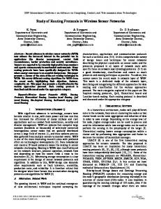
Figure 2. Ideal case, 1 BS in the center of the grid

Figure 3. Almost ideal case, 1 BS very close to the center of the grid The traditional routing tree construction works as follows. The BS broadcasts the initial MAKE TREE message to construct the tree and all the nodes choose a parent and broadcast the message further, until all nodes are reached, and the tree hierarchy is organized. In the case of Fig. 2, only 3 time steps are needed for all the nodes to hear the message and organize in the tree hierarchy. However, physically placing the BS in the exact center of the grid is usually a very hard thing to do and in most cases it will simply end up at a location very close to the center of the grid, like in Fig. 3. As shown in the figure, only a slight variation in the location of the BS induces an increase in the number of levels of the tree and therefore in the time it takes to construct the tree and to report the results. If the grid is bigger than 5*5, then the difference between the ideal case and the almost ideal case is more dramatic. Having a single routing tree does not provide any fault tolerance and also does not have any obvious benefits unless we find the exact center of the grid. If the grid has

an even number of nodes, than there is no exact center of the grid. Furthermore, our vision is that the BSs should be placed near the borders of the grid, so that they can be retrieved and replaced easily if needed. Before running any tests, our initial intuition was that more BSs should improve the performance of the system in all cases. However, we found that this does not hold. If we take the example in Fig. 4, we can easily see that it takes an extra 2 time steps to construct the trees!

Another interesting result was the fact that in the simulation, exactly like in real-life, not everything is perfectly synchronized and some nodes broadcast sooner than their peers. If we take into consideration Fig. 7, we can see that even though the BSs are placed in good locations and theoretically it should take the system 3 time steps to construct the trees, in reality it might take 4 time steps. We refer to the policy where the nodes choose their parent to be the first node their hear from, as the First Heard From policy (FHF). It is well known that FHF is not the best policy for a node to choose its parent, other criteria like the node with highest level of energy or fewest number of children are more efficient [13]. However, if the FHF policy is applied, than the behavior expressed above can take place.

Figure 5. Two BS placed in the middle of the borders of the grid This result made us question which can be the best and worst placement of the BSs and how the number of BSs affects the results.

Figure 4. Two BS placed in the corners of the grid

2.3

Analytical Examination

Continuing our study, we found that if we place two BSs in the middle of the borders of the grid facing each other, then we can get the same time steps necessary for constructing the trees as in the ideal case with one BS in the center of the grid (Fig. 5). After extensive experiments we came to the conclusion that 3 is the best number of time steps we can get regardless of the number of BSs in the network or their locations around the borders. We concentrate our attention around the borders of the grid because we want to be able to access the BSs quickly in case of any failure. The next challenge we wanted to solve was to derive formulas that would give us the time it takes for a given number of BSs to construct the routing trees. Fig. 6 shows the results for that.

Figure 6. Time necessary to construct the routing trees If we place a single BS randomly in the grid, the number of steps necessary to construct the routing tree is: max{max[N −1−Xbs , Xbs ], max[N −1−Ybs , Ybs ]}+1 where Xbs and Ybs are the X and Y coordinates of the BS in an N ∗ N grid. In the experiments section we discuss in more detail the tradeoffs involved in having different configurations of the BSs.

Figure 7. A single broadcast domain We illustrate this with an example, where we follow the execution of the FHF policy on an 5*5 grid of sensor nodes with two BSs (Fig. 7). Time step 1: - MAKE TREE message sent to BS, Node 10 and Node 14 Time step 2: - Node 10 (BS) broadcasts to Node 5, Node 6, Node 11, Node 15 and Node 16 - Node 14 (BS) broadcasts to Node 8, Node 9, Node 13, Node 18 and Node 19 Time step 3: - Node 5 broadcasts to Node 0 - Node 6 broadcasts to Node 1, Node 2, Node 7 - Node 11 broadcasts to Node 12 - Node 16 broadcasts to Node 17, Node 21, Node 22 - Node 15 broadcasts to Node 20 - Node 9 broadcasts to Node 4 - Node 8 broadcasts to Node 3, Node 2, Node 7 - Node 18 broadcasts to Node 17, Node 23 - Node 19 broadcasts to Node 24 Time step 4: - Node 21 broadcasts to Node 22 In the end, every node broadcasts the MAKE TREE message. When this message arrives at the 8 neighboring nodes, it is a different matter. In this example, the extra time step appears because Node 22 hears the MAKE TREE message first from Node 21 and not from Node 16 or Node 18 and once it chooses a parent, it does not reconsider other options and remains on level 3 in the first routing tree. This is how the standard Cougar protocol [11] works.

After selecting a parent, the sensor hears other “advertisements” from other sensors. Instead of dropping the rest of the messages, the node reads them and if the message proposes a lower level than the sensor is actually in, then it should select the sender of the message to be its parent and change its level to the new one. In Cougar, the sensor does not need to inform its children that it switched to a lower level and that in fact, the children themselves are in a better position, because the routing protocol is still working. We advocate using this kind of “need to know basis” parent selection, because it avoids long chains of sensors, creates better balanced trees and does not incur any extra costs. Of course there is no need for informing your parent that you are its child, it will figure it out after the first round of values transmitted towards the BS. If for any reason the sensors need to know their tree ID, then the sensors are still able to reselect their parent, but only within the initial selected tree. Otherwise, the node has to inform its children about the new tree ID. Due to space limitations we are not going to show the graphs for this case, but the experiments performed show that the performance of this case is very close to the previous one.

3

Experiments

In this section we first present our simulation environment and then give the details of our performance metrics. Lastly, we present the results of our experiments.

does not receive any reading from the network. In this case we cannot afford to do the tree reconstruction very often, and when we do so, we risk to miss important events or to have a big time gap among the sensor readings. Finally, if long-life is the primary goal of our network and we do not require very accurate results, then it is crucial to spend only a small amount of energy for the construction (reconstruction) of the routing trees. There is no point in performing an expensive tree reconstruction and then having only a few accurate sensor readings from the network afterwards, as the network would already have been drained out of energy.

3.2

Experiments and Results

3.2.1

Time steps necessary to construct the routing trees

We observed that placing the BS in the middle of the borders of the grid gives a very good time to construct the trees. From two BSs and up it is as good as the case with one BS in the center of the grid (Fig. 18 and Fig. 21). On the other hand, placing the BSs in the corners of the grid is never better than the middle of the borders placement, though it does improve when the FHF policy is applied.

3.2.2

Distribution of nodes per level 200

200

Simulation Environment and Performance Metrics

150 140 120

Nodes

We created a simulation environment using CSIM [14], based on Cougar [11]. Due to space limitations, we are going to show only the results for the 45*45 network, the rest of the simulations on different size networks being similar. For collision avoidance, we used in our simulation a contention-based MAC protocol (PAMAS) [15]. In this protocol, a sender node will perform a carrier sensing before initiating a transmission. If a node fails to get the medium, it goes to sleep and wakes up when the channel is free. We used several metrics in our evaluation: time steps necessary for the trees construction to finish, energy consumption, maximum and average number of nodes per level. Energy consumption includes the transmitting and listening energy. We do not take into account the sampling and processing energy, as their values are much smaller and are comparable in all schemes. We want to show that having several routing trees gives us the advantage of quicker construction of the routing trees and no single point of failure for the BS, at low or no extra energy costs. Therefore it is a good idea to use several routing trees covering the same area as a single one. On the other hand, if the time to reconstruct the trees is long, then there will be a period of time when the user

Nodes/Level

160

Nodes

3.1

Nodes/Level

180

100

100

80 60

50 40 20 0

0 0

10

20

30

Level

40

0

10

20

30

40

Level

Figure 8. 1BS center

Figure 9. 1BS almost center All the results shown for this distribution refer to the ideal case. We wanted to see what is the distribution of nodes per level for different number of BSs and different placement too. We discovered that for one BS in the center (Fig. 8), we have only 23 levels, but most of the nodes are located at the terminal levels. Any minor variation of the location of the BS (Fig. 9) gives an important variation in the distribution of nodes per level as well. The best case is definitely with four BSs located in the middle of the borders of the grid (Fig. 13). It has the smallest number of levels and the tree is most balanced, with most of the sensors closer to the BSs.

3.2.3

Distribution of AVERAGE number of nodes per level for grid configuration

For the FHF case (Fig. 23), all the average numbers are smaller than in the ideal case. Also, in the FHF case, the

200

200

200 nodes/level

160 140

Nodes

Nodes

100

180

150

150

100

120

Nodes

150

Nodes

200 nodes/level

nodes/level

100

nodes/level

100 80 60

50

50

50

40 20 0

0 0

10

20

30

0

40

0

0

Level

10

20

30

10

20

40

30

0

40

0

10

20

Level

Figure 10. 1BS middle

Figure 11. Two BS middle

Figure 12. Three BS middle

200

200

200 nodes/level

nodes/level

180 160

150

150

150

40

Figure 13. Four BS middle

200

nodes/level

nodes/level

30

Level

Level

100

120

Nodes

100

Nodes

Nodes

Nodes

140

100

100 80

50

60

50

50

40 20 0

0

0 10

20

30

40

0

10

20

Level

30

0

40

10

30

Figure 15. Two BS corner

Center

180

Figure 16. Three BS corner

Max # nodes per level

Middle of the borders Corners

140 120 100 80 60 40

Almost center

160

120 100 80 60 40 20

0

0

1

2

3

4

Middle of the borders Corners

140

20

30

40

Figure 17. Four BS corner

180

Center Almost center

160

Middle of the borders Corners

140 120 100 80 60 40 20

2

3

1

4

2

3

4

Number of base stations

Number of base stations

Figure 19. Max # nodes per level (ideal case)

200

20

0 1

Number of base stations

Figure 18. Time it takes to construct the trees (ideal case)

10

200 Center

180

Almost Center

160

0

Level

200

200

0

40

Level

Level

Figure 14. 1BS corner

Time steps

20

Average # nodes per level

0

Figure 20. Average # of nodes per level (ideal case)

200

200

Max # nodes per level

Almost center

160

Time steps

180

Center

Middle of the borders Corners

140 120 100 80 60 40 20 0 1

2

3

4

Number of base stations

Figure 21. Time it takes to construct the trees (FHF cases)

Average # nodes per level

Center

180

Center

160

Almost center Middle of the borders

140

Corner

120 100 80 60 40 20 0

180

Almost center Middle of the borders Corners

160 140 120 100 80 60 40 20 0

1

2

3

4

Number of base stations

Figure 22. Max # nodes per level (FHF case)

1

2

3

4

Number of base stations

Figure 23. Average # of nodes per level (FHF case)

distributions for placements of BSs in the middle of the borders and in the corners are very close.

3.2.4

Distribution of MAX number of nodes per level for grid configuration

The behavior of the system in this case is very similar with the one observed for the distribution of average number of nodes per level. For both distributions (average number of nodes per level and maximum number of nodes per level), both FHF and ideal case (Fig. 19 and Fig. 22) show great improvement for placing the BSs in the middle of the borders or in the corners of the grid compared to center or almost center placements. So, even for a single BS in the network, placing it in the middle of the borders or in the corners of the grid gives us some gains. If we have more than one BS, then the time and energy overheads disappear, at least for the placement in the middle of the borders.

3.2.5

Total power used for trees construction

The distribution for energy consumption follows very closely the time distribution, as we can see in Fig. 24. Total power consumption

5 4.5 4 3.5 3 2.5 2 Center

1.5

Almost Center

1

Middle of the borders Corners

0.5 0 1

2

3

4

Number of base stations

Figure 24. Total power used for tree construction (ideal case)

4

Conclusions and Future Work

In this paper, we showed that it is preferable to use a system with multiple routing trees instead of a single routing tree that covers the same area. We have also shown that the best placement for four base stations (BSs), is to place each in the middle of the borders of the grid. An approximate location is still good, if we are not able to place the BS exactly in the middle of the borders. Placing the four BSs in the corners of the grid is not as good as placing them in the middle of the borders, but still gives important benefits. Our simulations showed that placing more than four BSs around the borders does not give any extra gains. As future work, we intend to develop a fault-tolerant routing protocol that takes advantage of the multiple routing trees, to ensure even more reliability in the system. Also, we plan to find ways for routing trees of different length to synchronize data communication.

Acknowledgments This work was funded in part by NSF grant ANI-0123705 and by a startup grant from the School of Arts and Sciences at the University of Pittsburgh.

References [1] S. Bhattacharya and T. Abdelzaher, Data Placement for Energy Conservation in Wireless Sensor Networks, Proc. 1st International Conference on Mobile Systems, Applications and Services, 2003. [2] J. Considine, F. Li, G. Kollios and J. Byers, Approximate Aggregation Techniques for Sensor Databases, Proc. 20th International Conference on Data Engineering, 2004. [3] B.J. Ko and D. Rubenstein. Distributed, Self-Stabilizing Placement of Replicated Resources in Emerging Networks. Proc. 11th IEEE International Conference on Network Protocols, 2003, 6-15. [4] B. Krishnamachari and S. Iyengar, Distributed Bayesian Algorithms for Fault-Tolerant Event Region Detection in Wireless Sensor Networks, IEEE Transactions on Computers 53(3), 2003. [5] S. Madden, M. Franklin, J. Hellerstein, W. Hong, The Design of an Acquisitional Query Processor for Sensor Networks, Proc. 2003 ACM SIGMOD International Conference on Management of Data, 2003, 491-502. [6] S. Shenker, S. Ratnasamy, B. Karp, R. Govindan, D. Estrin, Data-centric storage in sensornets, ACM SIGCOMM Computer Communication Review 33(1), 2003, 137-142. [7] T. Stathopoulos and D. Estrin, An Information-Driven Reliability Mechanism for Wireless Sensor Networks, CENS Technical Report 16, 2003. [8] J. M. Younis, M. Youssef, K. Arisha, Energy-aware routing in cluster-based sensor networks, Proc. 10th IEEE International Symposium on Modeling, Analysis, and Simulation of Computer and Telecommunications Systems, 2002. [9] C. Intanagonwiwat, R. Govindan, D. Estrin, Directed Diffusion: A Scalable and Robust Communication Paradigm for Sensor Networks, Proc. 6th Annual International Conference on Mobile Computing and Networking, 2000. [10] S. Madden, R. Szewczyk, M. J. Franklin and D. Culler, Supporting Aggregate Queries Over Ad-Hoc Wireless Sensor Networks, Proc. 6th IEEE Workshop on Mobile Computing Systems and Applications, 2002. [11] Y. Yao and J. Gehrke, The Cougar Approach to InNetwork Query Processing in Sensor Networks, ACM Sigmod Record, 31(3), 2002, 9-18. [12] S. Madden, M. J. Franklin, J. M. Hellerstein and W. Hong, TAG: A Tiny Aggregation Service for Ad-Hoc Sensor Networks, Proc. 5th Annual Symposium on Operating Systems Design and Implementation, 2002. [13] J. Beaver, M. A. Sharaf, A. Labrinidis, P. K. Chrysanthis, Location-Aware Routing for Data Aggregation in Sensor Networks, Proc. Geo Sensor Networks, 2003. [14] H. Schwetman, CSIM Users Guide, MCC Corp., 1992. [15] S. Singhand and C. Raghavendra, PAMAS: Power Aware Multi-Access Protocol with Signalling for Ad Hoc Networks, ACM SIGCOMM Computer Communication Review, 28(3), 1998.