Multiple regression model for quantile functions

How to cope with modelling and privacy concerns? A regression model and a visualization tool for aggregated data

Rosanna Verde ([email protected]) Antonio Irpino ([email protected]) Dominique Desbois ([email protected]) Second University of Naples – Dept. of Political Sciences “J. Monnet”

1 of 30

Motivations and aims of the talk Motivation

• Regulation of official statistical institutes does not allow the diffusion of microdata for privacy-related purposes. In general, it is easier to obtain aggregated data of a set of individuals. • Most of the modelling tools in statistics (e.g., regression) work on microdata and cannot be easily extended to macrodata.

Methods

• In this talk, we show the use of a regression method developed for aggregated data, where both the explanatory and the response variables present quantile distributions as observations. • A PCA method on quantile data is used in order to visualize relationships between the predicted distributions.

Application

• The analysis has been performed on a dataset of economic indicators related to the specific cost of agriculture products in France regions. How to cope with modelling and privacy concerns? A regression model and a visualization tool for aggregated data R. Verde, A. Irpino, D. Desbois

2 of 30

DATA We observed data coming from RICA, the French Farm Accounting Data Network (FADN), aggregated in 22 metropolitan regions of France. CODE REGION 121 Île de France 131 Champagne-Ardenne 132 Picardie 133 Haute-Normandie 134 Centre 135 Basse-Normandie 136 Bourgogne 141 Nord-Pas-de-Calais 151 Lorraine 152 Alsace 153 Franche-Comté

How to cope with modelling and privacy concerns? A regression model and a visualization tool for aggregated data R. Verde, A. Irpino, D. Desbois

CODE REGION 162 Pays de la Loire 163 Bretagne 164 Poitou-Charentes 182 Aquitaine 183 Midi-Pyrénées 184 Limousin 192 Rhônes-Alpes 193 Auvergne 201 Languedoc-Roussillon 203 Provence-Alpes-Côte dAzur 204 Corse

3 of 30

Economic indicators available for each region o o o o

Y_TSC – Total Specific Cost (TSC) of farm holdings, X_WHEAT – the wheat output variable; X_PIG – the pig output variable; X_MILKC - the cow milk output variable;

The available data o Each region is described by the vector of the estimates of the 10 deciles of the distribution observed for each French region; Not-available information (for privacy concerns) o Raw data are not available: for each farm we do not know data about the four variables o We do not know association structure within each region o We do not know the number of farms observed for each region


4 of 30

An example of a row of the data table Y_TSC

CDF_Plot

Bretagne

Histogram

Bretagne

Smoothed histogram

Bretagne


X_Wheat

X_Pig

X_Cmilk

5 of 30

The data table: CDFs (Cumulative distribution functions) and corresponding histograms


6 of 30

A first research question? It is possible to predict Y_TSC from the other variables

Classic methods of regression cannot be used with this kind of data Proposal

• We may use Histogram-valued data analysis – – –

The regression for quantile functions: Verde-Irpino regression With each quantile function is associated a distribution Irpino-Verde regression is a novel method for the regression analysis of distributional data.


7 of 30

A regression model for histogram variables based on Wasserstein distance

8 of 30

A Regression model for histogram data Data = Model Fit + Residual Linear regression is a general method for estimating/describing association between a continuous outcome variable (dependent) and one or multiple predictors in one equation. Easy conceptual task with classic data But what does it means when dealing with histogram data? 0,5

0,45 0,4

0,4 0,3

0,3

0,3 0,2 0,2

0,15 0,1

0,1

0,1

Billard, Diday, IFCS 2006 Verde, Irpino, COMPSTAT 2010; CLADAG 2011 Dias, Brito, ISI 2011

0 0-10

1020

2030

3040

4050

5060


6070

7080

8090

90100

9 of 30

Linear Regression Model for histogram data (Verde, Irpino, 2013)

Given a histogram variable X, we search for a linear transformation of X which allows us to predict the histogram variable Y For example: given the histogram of the Y_TSC observed in a region, is it possible to predict the distribution of the Y_TSC using a linear combination of the predictor histogram variables?


10 of 30

Multiple regression model for quantile functions

Our concurrent multiple regression model is: p

yi ( t ) = β 0 + ∑ β j xij (t ) + ε i (t ) in matrix notation:

j =1

Quantile functions associated with histogram/ distribution data

= Y (t ) X (t ) β + ε (t ) This formulation is analogous to the functional linear model (Ramsay, Silverman, 2003) except for the constant

β parameters and for the

yi(t), xij(t) which are quantile functions while each εi(t) is a residual function (distribution?)

functions


for all i=1, …, n.

11 of 30

Parameters estimation - LS method using Wasserstein distance According to the nature of the variables, for the parameters estimation, we propose to extend the Least Squares principle to the functional case using a typical metric between quantile functions: 2

p   2 ε i ( yi ( t ), ˆyi (= t )) ∫  yi ( t ) − β 0 − ∑ β j xij ( t )  dt   j =1 0  1

(

1

) ∫(

d W2= xi ,x j

)

2

Fi −1( t ) − F j −1( t ) dt

0


Squared error based on the Wasserstein l2 distance between two quantile functions

Wasserstein l2 distance between two quantile functions

12 of 30

Fitting linear regression model Find a linear transformation of the quantile functions of xij (for j=1,…,p) in order to predict the quantile function of yi i.e.: p

yî (t ) = β 0 + ∑ β j xij (t ) ∀t ∈ [0,1] j =1

The linear transformation is unique: the parameters β0 and βj are estimated for all the xij and yi distributions A first problem:

Only if βj > 0 a quantile function yˆ i (t )can be derived.

In order to overcome this problem, we propose a solution based on the decomposition of the Wasserstein distance and on the NNLS algorithm. How to cope with modelling and privacy concerns? A regression model and a visualization tool for aggregated data R. Verde, A. Irpino, D. Desbois

13 of 30

OLS estimate (Irpino and Verde, 2012) The quantile function can be decomposed as:

xij (t ) = xij + xijc (t ) where

c x= xij (t ) − xij is the centered quantile function ij (t )

Then, we propose the following regression model: p

p

yi (t ) = β 0 + ∑ β j xij + ∑ γ j xijc (t ) + i (t ) 0 ≤ t ≤ 1 =j 1 =j 1  yî ( t )

Using the Wasserstein distance it is possible to set up a OLS method that returns the two sets of coefficients (β0,βj; γj). Under a positiveness constraint on γj


14 of 30

Interpretation of the parameters Regression parameters for the distribution mean locations

βˆ0 , βˆ1 ,..., βˆ p ∈ℜ Shrinking factors for the variability

γˆ1 ,..., γˆ p ∈ℜ+

> 1 (< 1) the yî histogram has a greater (smaller) variability than the xij histogram.


15 of 30

Advantages of the regression on quantile functions • The regression on quantile functions takes into account the whole distribution (described by the quantiles). • It is more powerful with respect a classic regression on the means of the distributions because it considers information about sizes and shapes of the distributions. • It is different from the well-know Quantile regression which requires all microdata and estimates one quantile at time (independently from the others). In this case it is not guaranteed the order among the estimated quantile. • Our methods works on aggregated data when microdata are not available, and estimates the quantiles using a single model. The method guarantees the natural order among the estimated quantiles. • The method suffers less of the outlying observations, thus it guarantees a more robust estimation of the tails of the distributions.


16 of 30

Regression results

(only the first 19 regions are used, the last three have regressors equal to zero)

The estimated model 16,834.4 + Y _TSCi (t ) =

0.6671 ⋅ X _ WHEAT i

+0.7793 ⋅ X _ WHEATi c (t )

0.6095 ⋅ X _ PIG i

+0.5478 ⋅ X _ PIG (t )

0.2651 ⋅ X _ MILKC i

+0.3438 ⋅ X _ MILKCic (t )

Goodness of fit indices Root Mean Square Error (Verde & Irpino, 2013): Omega index (Dias & Brito, 2011): Pseudo R-squared (Verde & Irpino, 2013):


c i

t ∈ [0;1]

RMSE=7,238.2; Ω =0.9069 (0 worst fitting, 1 best fitting); PR2 =0.7233 (0 worst fitting, 1 best fitting).

17 of 30

Plot of observed CDFs vs predicted CDFs

Observed Predicted


18 of 30

Plot observed vs predicted (zoom)


19 of 30

A visualization tool for distributions Motivations A distribution, being a function, is a high dimensional data. We observed the plots in the last two slides: • This kind of visualization is not very communicative. • It is difficult to compare different distributions visually. We need a visualization tool that organizes graphically the distributions according to a similarity criterion. A new visualization tool: Quantile PCA (Irpino and Verde, 2013) Chosen a fixed number of quantiles, Quantile PCA performs a principal component analysis on a single distributional variable (a column of the data table).


20 of 30

PCA of quantiles The X matrix decomposed in Q-PCA • We fix a set of m quantiles • Each individual is represented by a sequence of m+1 (including the minimum value) ordered values

xi = min(xi ) Qi 1 … Qij … Qi ,m−1 Max(xi )  min(x1 ) Q1,1  … …  X =  min(xi ) Qi ,1  …  … min(xN ) QN ,1  How to cope with modelling and privacy concerns? A regression model and a visualization tool for aggregated data R. Verde, A. Irpino, D. Desbois

… Q1, j … … Qi , j

… Q1,m−1 … … … Qi ,m−1

… … … … … QN , j … QN ,m −1

Max(x1 )  …  Max(xi )   …  Max(xN )

21 of 30

Average quantiles vector The m+1 quantile column variables are centered

X=

 min(x1 ) Q1,1  … …   min(xi ) Qi ,1  …  … min(xN ) QN ,1 

… Q1, j … … Qi , j … … … QN , j

… Q1,m−1 … … … Qi ,m −1 … … … QN ,m −1

Max(x1 )  …  Max(xi )   …  Max(xN )

−

x� = min(x) Q1 …

Qj …

Qm −1

Max(x)

X – IN • x = Xc with IN the unitary vector of N elements

Average quantiles

A PCA on the variance-covariance matrix of quantiles is performed. Note: the trace of the covariance matrix is an approximation of a variance measure defined for a distributional-variable. How to cope with modelling and privacy concerns? A regression model and a visualization tool for aggregated data R. Verde, A. Irpino, D. Desbois

22 of 30

Eigenvalues and explained inertia Wasserstein-based Variance of the variable Y_TSC = 2.5318x108 ; Trace of the quantile Variance-Covariance matrix = 2.7815x108.


Eigenvalues

E1 E2 E3 E4 E5 E6 E7 E8 E9

Inertia 2.5739 x108 0.1702 x108 0.0223 x108 0.0095 x108 0.0027 x108 0.0015 x108 0.0007 x108 0.0005 x108 0.0001 x108

% of explained % cum 92.54 92.54 6.12 98.66 0.80 99.46 0.34 99.80 0.10 99.89 0.05 99.95 0.02 99.97 0.01 99.98 0.006 100.000

E1 E2

2,57E+08

1,70E+07

E3

2,23E+06

E4

9,50E+05

100

E5

2,70E+05

98

Cum. perc. of explained inertia

96 94 92 90 88

E1 E2 E3 E4 E5 E6 E7 E8 E9 Eigenvalues

23 of 30

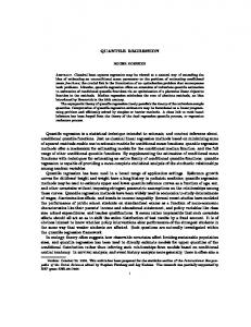
The plot of variables: the Spanish-fan plot Median Upper quantiles

Lower quantiles


Comment: Great part of variability is due to differences on the right tail. (Right-skewness)

24 of 30

Principal Component Analysis of the Y_TSC variable: First factorial plane


25 of 30

PCA of the Y_TSC variable: First factorial plane (distribution colored according to the means)

Higher mean

Lower mean


26 of 30

PCA of the Y_TSC variable: First factorial plane

(distribution coloured according to standard deviations)

Lower std Higher std


27 of 30

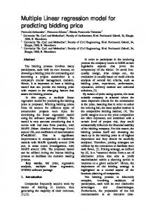
PCA of the Y_TSC variable: First factorial plane a joint view

Comment: means and stds seems slightly positive correlated, they are both related to right heavy tailed distributions


28 of 30

Conclusions •

In this talk, starting from aggregated data, and without knowing microdata, we showed that it is possible to analyze, predict and show such summary structures using new tools from distributional-valued data analysis, defined into a space of univariate distributions equipped with L2 Wasserstein metric.

•

A regression technique is able to work with this kind of data and it provides accurate and interpretable (also for practitioners) results for the interpreting of the causal relationships.

•

A PCA on quantiles is a promising tool for a fast and easy visualization of the different distribution features.

•

An R package is going to be released in the next quarter.

As a future work, a graphical analysis of predicted vs observed distribution-valued data can be introduced using more sophisticated factorial analysis. (This is in progress)


29 of 30

Main references 1. Arroyo, J., Maté, C.: Forecasting histogram time series with k-nearest neighbors methods, International Journal of Forecasting 25 (1), 192-207 (2009) 2. Arroyo, J., González-Rivera, G., Maté C.: Forecasting with interval and histogram data. Some financial applications. Handbook of empirical economics and finance, 247-280 (2010) 3. Dias, S., Brito, P.: A new linear regression model for histogram-valued variables, in: 58th ISI World Statistics Congress, Dublin, Ireland, URL: http://isi2011.congressplanner.eu/pdfs/950662.pdf, (2011) 4. Irpino, A., Verde, R.: Dimension reduction techniques for distributional symbolic data. In: SIS 2013 Statistical Conference Advances in Latent Variables - Methods, Models and Applications. URL: http://meetings.sis-statistica.org/index.php/sis2013/ALV/paper/viewFile/2586/443 (2013) 5. Irpino, A. Verde, R. : Ordinary Least Squares for Histogram Data Based on Wasserstein Distance. In: COMPSTAT’2010, 19th Conference of IASC-ERS (Physica Verlag), pp. 581-589 (2010). 6. Irpino, A., Verde, R.: Basic statistics for distributional symbolic variables: a new metric-based approach. Advances in Data Analysis and Classification, doi: 10.1007/s11634-014-0176-4 (in press, 2015) 7. Rüschendorf,, L.: Wasserstein metric, in Hazewinkel, M., Encyclopedia of Mathematics, Springer (2001) 8. Verde, R, Irpino, A.: Multiple Linear Regression for Histogram Data using Least Squares of Quantile Functions: a Two-components model. Revue des Nouvelles Technologies de L'Information, vol. RNTIE-25, p. 78-93 (2013)


30 of 30


Thanks For Listening Antonio Irpino, Rosanna Verde, Dominique Desbois, November 25th, 2014

31 of 30

Multiple regression model for quantile functions

Multiple regression model for quantile functions

Suggest Documents

Dynamic Model Averaging for Bayesian Quantile Regression

Testing Equality of Nonparametric Quantile Regression Functions

Quantile Regression on Quantile Ranges

QUANTILE REGRESSION

vgam Family Functions for Quantile Regression - Semantic Scholar

Wild bootstrap for quantile regression

Development of Multiple Regression Functions for Performance ...

Quantile Regression on Quantile Ranges

A Quantile Regression Approach

Nonparametric Quantile Regression

Bayesian Robust Quantile Regression

Quantile Regression - Google Sites

Nonparametric Quantile Regression

A Quantile Regression Approach

Multiple-regression hospitalization-cost model for ...

Multiple-regression hospitalization-cost model for ...

Fuzzy Multiple Regression Model for Estimating Software ...

Multiple Linear regression model for predicting ...

Non-crossing quantile regression curve estimation - Multiple Choices

Alternative configurations of quantile regression for estimating ...

Local bilinear multiple-output quantile/depth regression - arXiv

Quantile regression models for fish recruitment–environment ...

Consistent Specification Testing for Quantile Regression ... - CiteSeerX

Poinrwise adaptive estimation for quantile regression - Humboldt ...