model that can predict the bidding price with respect ... developing the linear regression model using the .... simple linear models, with one independent variable.
Multiple Linear regression model for predicting bidding price Petrovski Aleksandar1, Petruseva Silvana 2, Zileska Pancovska Valentina3 1 University “Ss. Cyril and Methodius“, Faculty of Architecture, Blvd. Partizanski Odredi, 24, Skopje, 1000, R. Macedonia 2 University “Ss. Cyril and Methodius“, Faculty of Civil Engineering, Blvd. Partizanski Odredi, 24, Skopje, 1000, R. Macedonia 3 University “Ss. Cyril and Methodius“, Faculty of Civil Engineering, Blvd. Partizanski Odredi, 24, Skopje, 1000, R. Macedonia
Abstract The bidding process involves many participants, each with its own interest, so choosing a bidding price for contracting and becoming a project stakeholder is a company's crucial management decision. Hence, it is important to have a bidding model that can predict the bidding price with respect to the changing factors that attack the bidding process. In this paper, a multiple linear regression model for predicting the bidding price is proposed. Winning bidding prices from 26 tenders for different types of construction projects were input for developing the linear regression model using the software package DTREG. The model is very accurate considering that it works with real data from practice, with MAPE (Mean Absolute Percentage Error) around 3%, and coefficient of determination This is significant R2=0.88167. improvement in comparison to traditional models with MAPE typically around 25% and, in some recent investigations, with MAPE around 19%. The proposed model can be utilized during the intense bidding process to facilitate the decision making process. Key words: bid price, regression analysis, multiple linear regression, DTREG software package 1. Introduction Companies frequently acquire work by means of bidding in tenders, thus generating the majority of their revenues, [1],[2].
In order to participate in the tendering process the company needs to fulfill certain legislative aspects that prove the competency of the bidder. To avoid lowquality design, time delays etc., the evaluation is usually based on multi-criteria analysis of several bid criteria, such as bidding price, experience, performance, reputation, delivery method and technical solutions, [3]. By means of point rating system, the most suitable company is selected where the most important criteria for the commission is the price, meaning that in order to select the winning bid, the most applied method is the competitive bidding method, [4]. The profit margins due to the price competition are often depressed, and combined with a certain level of project risk, they could substantially influence the financial stability of the bidding company. For this reason, the bidding process itself and choosing the mark-up in the bidding price is of highest importance and they should be carefully analyzed. Therefore, pricing strategies are utilized by the contractors to facilitate their cash flows, [5]. Pricing strategy, as defined by [6], is a “reasoned choice from a set of alternative prices that aim at profit maximization within a planning period in response to a given scenario”. Hence, the importance of the bidding strategy is highlighted as a crucial aspect of the business planning of companies. The bidding process is inherently complex, involving multitude of participants, each with its own distinctive advantages and disadvantages. Furthermore, the preparation of the bid documentation is an intensive time-
consuming and costly process including broad research on a number of internal or external aspects, [7],[8]. During the bid preparation, the company is due to reevaluate its resources and capacity for a sustainable project delivery. Usually, the bidding decisions are propped by the contractor’s experience, intuition and personal bias, [5],[9]. The calculation of the bidding price comprises of direct cost (such as labor, crew, materials, equipment, subcontractors etc.), indirect costs (like project overhead, equipment, human resources) and the markup amount such as contingency, profit, risk allowance and general overhead. Therefore, the need for a better technique for decision making is stressed by several authors, [10],[8]. It is important to have a bidding model that can predict the dynamic bidding process with respect to changing price in order to win the bid. The development of linear regression in order to predict the cost of construction in buildings was described by [11]. They obtained model with MAPE (Mean Absolute Percentage Error) around 19% and R2=0.661, which compare favorably with the past research which has shown that the traditional methods of cost estimation typically have MAPE around 25%. The aim of this research is to develop a predicting model that can be utilized during the intense bidding process and to facilitate the decision making process. In this paper we obtained a predictive linear regression model using DTREG software package, with MAPE around 3% and R2= 0.88167 which can be considered as very accurate predicting, having in mind that the model uses data from real practice. In the next section several bidding strategies are reviewed, followed by the proposed methodology. 2. Literature review Potential factors that affect the bidder decision are numerous. Bagies and Fortune, [10] have identified them using different techniques such as parametric, utilitytheory, artificial neural network, fuzzy
neural network, fuzzy logic and regression techniques intended for mark-up models determination. It is concluded that the listed techniques could be beneficial for facilitating the bid decision, [10]. Many authors have scrutinized different decision making models based on artificial intelligence (AI), such as the expert system [12], case-based reasoning [13], neural network [14], analytical hierarchy process [15] and fuzzy set theory [16],[17]. In the scientific environment different bidding models have been examined such as: game-theory models, statistic models including expected monetary-value based and expected utility value based, as well as cash flow based. The most commonly used models for probability determination of winning, against a number of competitors and mark-up calculation are the Gate’s and Friedman’s model, [18]. Classification of bidding strategies is made into three categories, [14]: models based on probability theory by Friedman [19] and Gates [20], directed towards expected profit maximization, models based on decision-support systems [12] which consider the multi-attribute nature of bidding decisions and emerging models based on artificial intelligence [21]. The Friedman’s models utilization is reexamined by many authors, concluding that the results are unsupportive of the decision making process, especially in symmetrical situations when competitors have equal winning chances. Competitive bid could be conducted by means of closed bidding process or incremental bidding until none of the bidders increases the bid. The method determines the optimal bidding price based on the distribution of the ratio of the bidding price to cost estimate. Friedman states that some of the simpler bidding problems can be solved by gametheory techniques, [19]. Seven bidding strategies have been proposed by Gates that intend to optimize the profit of the bidder, [20]. This model provides direct calculation of the probability. The model is argued by Skitmore et. al, [22], stating that for the
Gate’s method utilization a Weibull distribution of the bids is required. Further, studies have been undertaken on generic software bidding model for estimating the probability of a successful method, [23]. Sonmez [24], presents an approach for integration of parametric and probabilistic cost estimation techniques using a combination of regression analysis and bootstrap resampling technique in order to develop range estimates for construction costs. For facilitating the bidding strategy King and Mercer proposed a methodology in which, in the absence of sufficient detailed price data, the market lower bid strategy was determined as precisely allowing simulation of possible strategy changes [25]. Probability distributions for bidders information development is a common case widely adopted in the state-of-the-art literature and often unfeasible in practice, [26],[2]. Cagno [15] described Analytic Hierarchy Process (AHP) assessing the probability of winning a competitive bidding process where competing bids are evaluated on a multiple criteria basis. Reeves et al. [27] stress the difficulty of drawing conclusions about strategy choices in a relatively simple simultaneous ascending auction game. The analytic methods are not fruitful due to the large space of strategies causing large simulation studies to be out of question. MacKie et. al. enabled final price prediction and performance, by employing empirical game-theoretic methodology and establishing Nash equilibrium profiles for restricted strategy sets [28]. Regarding the previously stated, in the next section of this paper a model for prediction and support of the bid decision process is presented, utilizing a linear regression technique. 3. Methodology Data from 52 tenders for different types of construction projects were collected during 2014 from firms in FYR of
Macedonia, financed by public funds. Only the winning bidding data for 26 structures were the contracts that were signed and were used for further analyses. The collected data covered information about: the structures’ type, purpose of construction, place of construction, bidding price, winning price, year of the contract, and problems that have occurred for the firm during the bidding process. They were input in the DTREG software package [29] for creating the linear regression model for bidding price prediction. In the next section we shall give short overview of the linear regression method and after that the predictive model will be presented, using DTREG software. 4. Research 4.1. Linear regression The statistical process for estimating the relationship between different variables is called regression analysis. Regression analysis is being widely investigated in the area of machine learning for prediction. Regression analysis is used to understand how the value of the dependent variable changes when one of the independent variables changes, while other variables are fixed. Most often, regression analysis is used for computing the average value of the dependent variable when the independent variables are fixed. Many techniques for researching regression analysis have been developed, which can generally be divided in parametric and non-parametric. Linear regression is a parametric method where the dependent variable (regression function) is defined with a finite number of unknown parameters that are computed from the independent variables. Non-parametric techniques allow regression function to be a function which may be infinite dimensional. Linear regression (LR) is a statistical method which models the relationship between dependent (or response) variable Y and one or more explanatory (or independent) variables x. The function Y is called regression function.
Every value of the independent variable x is associated with a value of the dependent variable Y. The regression function Y dependent on n explanatory (predictor) variables x1, x2,.., xn is given with eq. (1)
Y = β0 + β1x1 + β2x2 +......+ βn xn
(1)
If there exists an exact fit between the real data and the regression (predicted) function, then the actual data would be equal to the predicted values. But, of course, this is not the case, and there is a difference between the actual value of target variable and its predicted value, and this difference is the error of the estimation which is called “deviation” or “residual”.
This equation describes how the mean response Y changes with the explanatory variables. β1 , β 2 ,......β n are unknown
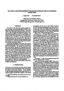
parameters (coefficients). β 0 is a constant. If the regression function is linear in the parameters (but not necessarily in the independent variables), we call it linear regression model. Otherwise, the model is called non-linear. Linear regression (LR) models with more than one independent variable are called multiple linear models, as opposed to simple linear models, with one independent variable. Linear regression rarely works as well on real-world data, as more general techniques such as neural networks which can model non-linear functions, because it fits linear (straight line/plane) functions to the input data. But, linear regression has many practical uses and a number of advantages. For example, linear regression is well understood, and training linear regression model is much faster that other predictive models, like neural networks. Also LR can be applied to compute the strength of the relationship between Y and the xj, to compute which xj may have no relationship with Y at all, and to identify which subsets of the xj contain redundant information about Y. Moreover, LR models are very simple and require minimum memory space for implementation, so they work well on controllers with limited memory space. If in a LR model there is only one independent variable x1, then the regression function is a straight line, if there are 2 independent variables, then the regression function is a plane; and for n predictor variables the dependent function is ndimensional hyper-plane. In Figure 1 [30] we have a plane fitted with 2 predictors.
Figure 1. Fitted plane with 2 predictors
The goal of LR is to compute the values of parameters so that the sum of squared residual values for the set of observations is minimal. This process is called “least squares” regression fit. By estimating the sign and value of the regression coefficients, we can infer how the predictors affect the target outcome. If our task is forecasting, then linear regression fits a predictive model to the input data set of y and xi values. After developing the model, if an additional value of xi is given, and its attendant value of y is not given, then we can use the fitted model for making a prediction of the value of y. 4.2. Multiple linear regression model for predicting bidding price using DTREG For creating the multiple linear regression model for predicting of the bidding price for the 26 structures, DTREG software package was used [30]. DTREG uses robust Singular Value Decomposition
algorithm to perform linear regression. The results of the DTREG analysis of the model
are presented from Table 1 to Table 4.
Table 1. Input data Input data Target variable: ln(received price) Number of predictor variables: 2 Type of model: Linear regression Type of analysis: Regression Validation method: Cross validation Number of cross-validation folds: 10 ============ Input Data ============ Input data file: TENDERS Number of variables (data columns): 14 Data subsetting: Use all data rows Number of data rows: 26 Total weight for all rows: 26 Rows with missing target or weight values: 0 Rows with missing predictor values: 0 -Statistics for target variable: ln(received price) Mean value = 13.126042 Standard deviation = 1.5542198 Minimum value = 10.164312 Maximum value = 16.28361 ===== Summary of Variables ========== Number Variable Class Type Missing rows ------ ----------------------------------- --------- -1 number of project Unused Continuous 0 2 category of construction Unused Categorical 2 3 year of construction Unused Continuous 0 4 purpose of construction Unused Categorical 0 5 in Skopje Unused Categorical 10 6 outside Skopje Unused Categorical 6 7 price offered Unused Continuous 0 8 received an offer price Unused Continuous 0 9 contract signed or no Unused Categorical 0 10 time for preparing tender doc-days Unused Continuous 0 11 problems about the tender documen. Unused Categorical 9 12 ln (price offered) Predictor Continuous 0 13 ln(received price) Target Continuous 0 14 ln(time for prepar. doc) Predictor Continuous 0
Part of the data is used for training of the model (training data) (Table 3), and part of the data is used for validation of the model (validation data) (Table 4). The linear regression model has been implemented for 2 predictors. We shall stress here that the choice of the predictors is very important for accuracy of the model. Here, instead of numerical value of target variable and predictors, ln(target variable) and ln(predictors) is used, because more accurate prediction is obtained in this way.
Categories
25 8
For preparing of the variables of the multiple linear regression model, we used the Bromilow’ time-cost model [31]:
T = K1C1
B1
and T = K 2 C 2 B2
(2)
where T is the time of preparation of documents (in days), C1 is price offered and C2 is price received. K1, K2, B1 and B2 are constants which are being determined by the model. By logarithm of equations (2) we have
lnT=lnK1+B1lnC1
(3)
lnT=lnK2+B2lnC2
By summarizing (3) and (4), we have (eq.5): 2ln T= lnK1+B1lnC1 + lnK2+B2lnC2 (5) From equation (5), if we express lnC2, we receive the dependence of the price received C2 from the time of preparation of documents T and the price offered C1 (eq.6):
ln C 2 = (2ln T - lnK1 - B1lnC1 - lnK 2 )
1 B2
(6)
By putting in order eq. (6) we obtain our multiple linear regression model:
ln C 2 = β 0 + β1ln T + β 2 lnC1
(7)
where lnC2 is target regression function, lnT and ln C1 are predictor variables, which are input in the software package DTREG.
(4)
After learning the model, coefficients β 0 , β1 , β 2 are determined and we can put some new input values for T and C1 and we can receive prediction of lnC2. By antilogarithm of lnC2, we receive prediction of C2. Results for the model with 2 predictors are given in Table 4 for validation data. Here variable ln(received price) is used as target variable, and ln(price offered) and ln(time for prep doc) as predicted variables (Table 1). DTREG generates a table (Table 2) which shows the obtained coefficient values (for each predictor variable), in addition to the statistics on how well the regression function fits the data. Except for the coefficient values, the standard error of the coefficients and several other statistics are also displayed (Table 2).
Table 2. Computed coefficient beta values Linear Regression Parameters -------------- Computed Coefficient (Beta) Values -------------Variable Coefficient Std. Error t Prob(t) 95% Confidence Interval ----------------------------------- ------------ --------- --------- ------------ -----------ln (price offered) 0.953011 0.0631 15.11 < 0.00001 0.8225 1.083 ln(time for pre.doc) 0.0652043 0.121 0.54 0.59406 -0.1844 0.3148 Constant 0.210477 0.8779 0.24 0.81264 -1.606 2.026
The “t” statistics is obtained by dividing the computed value of the coefficient by its standard error. This statistics gives an estimation of the likelihood that the actual value of the parameter can be zero. The confidence interval is the range of values for the obtained coefficient value with the specified confidence, which means that we are 95% confident that the value of the coefficient falls in this range. For example, in our table we have that the coefficient 0.953011 is in the range of 0.8225 to 1.083 with confidence 95%. The ANOVA
(Analysis of Variance) (Table 3 and Table 4) shows statistics for the general significance of the regression model which is being fitted. The “F value” and “Prob (F)“ test the null hypothesis that all regression coefficients are equal to 0. Prob (F) is the probability that the null hypothesis for the full model is true (that all regression coefficients are 0) [30]. The accuracy of the model is estimated from the statistics of validation data (Table 4).
Table 3. Training data Analysis of Variance Mean target value for input data = 13.126042 Mean target value for predicted values = 13.126042 Variance in input data = 2.4155993 Residual (unexplained) variance after model fit = 0.2210897 Proportion of variance explained by model (R^2) = 0.90847 (90.847%) Coefficient of variation (CV) = 0.035822 Normalized mean square error (NMSE) = 0.091526 Correlation between actual and predicted = 0.953139 Maximum error = 1.6461913 RMSE (Root Mean Squared Error) = 0.4702018 MSE (Mean Squared Error) = 0.2210897 MAE (Mean Absolute Error) = 0.3486989 MAPE (Mean Absolute Percentage Error) = 2.6517839 -- ANOVA and F Statistics -Source DF Sum of Squares Mean Square F value Prob(F) ---------- ------ -------------- -------------- ---------- --------Regression 2 57.05725 28.52862 114.148