Multiple Sensor Image Registration, Image Fusion and Dimension Reduction of Earth Science Imagery Jacqueline Le Moigne NASA Goddard Space Flight Center Applied Information Science Branch Greenbelt, MD 20771
[email protected]
Arlene Cole-Rhodes, Roger Eastman, Tarek El-Ghazawi, Kisha Johnson, Sinthop Kaewpijit, Nadine Laporte, Jeffrey Morisette, Nathan S. Netanyahu, Harold S. Stone, Ilya Zavorin At the same time, on the ground, continuity of the data as well as extrapolation among several scales, temporal, spatial, and spectral, remain key components of many remote sensing applications, and these properties are provided by integration and seamless mosaicking of multiple sensor data, via image registration and fusion.
Abstract - The goal of our project is to develop and evaluate image analysis methodologies for use on the ground or on-board spacecraft, particularly spacecraft constellations. Our focus is on developing methods to perform automatic registration and fusion of multisensor data representing multiple spatial, spectral and temporal resolutions, as well as dimension reduction of hyperspectral data. Feature extraction methods such as wavelet decomposition, edge detection and mutual information are combined with feature matching methods such as cross-correlation, optimization, and statistically robust techniques to perform image registration. The approach to image fusion is application-based and involves wavelet decomposition, dimension reduction, and classification methods. Dimension reduction is approached through novel methods based on Principal Component Analysis and Wavelet Decomposition, and implemented on Beowulfstype parallel architectures. Registration algorithms are tested and compared on several multi-sensor datasets, including one of the EOS Core Sites, the Konza Prairie in Kansas, utilizing four different sensors: IKONOS, Landsat-7/ETM+, MODIS, and SeaWIFS. Fusion methods are tested using Landsat, MODIS and SAR or JERS data. Dimension reduction is demonstrated on AVIRIS hyperspectral data.
For both on-board and on-the-ground applications, the particular need for dimension reduction is two-fold, first to reduce the communication bandwidth, second as a pre-processing to make computations feasible, simpler and faster.
2
In this work, “image registration” is defined as a featurebased “precision correction,” in opposition to a modelbased “systematic correction.” In our experiments, we assume that the data has already been systematically corrected according to a navigation model. The goal of a precision-correction algorithm is to utilize selected image features or control points to refine the geo-location accuracy given by the systematic model within one pixel or a sub-pixel. Currently, there is a large quantity of potential image registration methods that have been developed for aerial or medical images and that are applicable to remote sensing images [1,2]. But there is no consolidated approach that enables a user to select the most appropriate method for a remote sensing application, given the type of data, the desired accuracy and the type of computational power available with respect to timing requirements. The intent of our work is to survey, design, and develop different components of the registration process and to evaluate their performance on well-chosen multi-sensor data.
Keywords: registration, fusion, dimension reduction, wavelet processing, remote sensing, hyperspectral.
1
Introduction
With the development of future spacecraft formations comes a number of complex challenges such as maintaining precise relative position and specified attitudes, as well as powerful communication capabilities. More generally, with the advent of spacecraft formations, issues related to performing on-board and autonomous data computing and analysis as well as decision planning and scheduling will figure among the most important requirements. Among those, automatic image registration, fusion and dimension reduction represent intelligent technologies that would reduce mission costs, would enable autonomous decisions to be taken on-board, and would make formation flying adaptive, self-reliant, and cooperative.
ISIF © 2002
Image Registration
2.1 Brief Image Registration Survey As a general definition, automatic image registration of satellite image data is the process that aligns one image to a second image of the same scene that was acquired at the same or at different times by different or identical sensors. One set of data is taken as the reference data, and all other data, called input data (or sensed data), is matched relative to the reference data. The general process of image registration includes three main steps:
999
1) extraction of features to be used in the matching process, 2) feature matching strategy and metrics, and 3) data resampling based on the computed deformation (sometimes replaced by indexing or fusion). Many choices are available for each of the previous steps [1,2]. Our work [3-11] has mainly been dealing with features such as gray levels, edges, and wavelet coefficients, and matching them using either crosscorrelation, Mutual Information or a Hausdorff distance as a similarity metrics, and exhaustive search or optimization techniques as search strategies.
2.2 Correlation-Based Experiments Our first experiments utilized cross-correlation as a similarity metrics, and features such as gray levels, edges, and Daubechies wavelet coefficients were compared using mono-sensor data [3]. Results showed that, as expected, edges or edge-like features like wavelets are more robust to noise, local intensity variations or time-of-the day conditions than original gray level values. On the other hand, when only looking for translation on cloud-free data, phase correlation provides a fast and accurate answer. Comparing edges and wavelets, orthogonal wavelet-based registration was usually faster although not always as accurate than a full-resolution edge-based registration. This lack of consistent accuracy of orthogonal wavelets seemed to be due to their lack of translation-invariance, and was studied in more details in the second set of experiments.
2.3 Wavelet-Based Experiments According to the Nyquist criterion, in order to distinguish between all frequency components and to avoid aliasing, the signal must be sampled at a frequency that is at least twice the signal's highest frequency component. Therefore, as pointed out in [12], “translation invariance cannot be expected in a system based on convolution and subsampling.” When using a separable orthogonal wavelet transform, information about the signal changes within or across sub-bands. By lack of translation (resp. rotation) invariance, we mean that the wavelet transform does not commute with the translation (resp. rotation) operator. To study the effects of translation and rotation, we conducted two studies: (1) the first study [10] quantitatively assessed the use of orthogonal wavelet sub-bands as a function of features’ sizes. The results showed that: • low-pass sub-bands are relatively insensitive to translation, provided that the features of interest have an extent at least twice the size of the wavelet filters. • high-pass sub-bands are more sensitive to translation, but peak correlations are high enough to be useful. (2) the second study [5] investigated the use of an overcomplete frame representation, the “Steerable Pyramid”. It was shown that, as expected and due to their translation- and rotation- invariance, Simoncelli’s steerable filters perform better than Daubechies’ filters. Rotation errors obtained with steerable filters were minimum,
1000
independent of rotation size or noise amount. Noise studies also reinforced the results that steerable filters show a better robustness to larger amounts of noise than do orthogonal filters.
2.4 Feature Matching Experiments All previous work focused on correlation-based methods used with an exhaustive search. One of the main drawbacks of this method is the prohibitive computation times when the number of transformation parameters increases (e.g., affine transformation vs. shift-only), or when the size of the data increases (full size scenes vs. small portions, multi-band processing vs. mono-band). To answer some of these concerns, we investigated different types of similarity metrics and different types of feature matching strategies. In this study, five different algorithms were developed and compared. The features that were utilized were original gray levels and wavelet features. The different metrics were correlation, mutual information [13] and a Partial Hausdorff distance [14]. The strategies were exhaustive search, optimization and robust feature matching. The five algorithms can then be described as follows: • Gray Levels matched by Fast Fourier Correlation Methods [15]. • Gray Levels matched by gradient descent [9] using a least squares criterion. • Simoncelli wavelet features matched by exhaustive search of the correlation maximum [5]. • Simoncelli wavelet features matched by exhaustive search of the mutual information maximum [11]. • Simoncelli wavelet features matched by robust feature matching using a partial Hausdorff distance [6,7]. See [8] for more details on each of these algorithms. The dataset used for this study represents multisensor data acquired by four different sensors over one of the MODIS Validation Core Sites. The site is the Konza Prairie in the state of Kansas, United States. The four sensors and their respective bands and spatial resolutions involved in this study are: 1) IKONOS Bands 3 (Red) and 4 (Near-Infrared), spatial resolution of 4 meters per pixel, 2) Landsat-7/ETM+ Bands 3 (Red) and 4 (Near-Infrared), spatial resolution of 30 meters per pixel, 3) MODIS Bands 1 (Red) and 2 (Near Infrared), spatial resolution of 500 meters,per pixel, 4) SeaWIFS Bands 6 (Red) and 8 (Near Infrared), spatial resolution of 1000 meters per pixel. Since most of the algorithms considered for this study do not yet handle scale, we initially re-sampled the IKONOS and ETM+ data to the respective spatial resolutions of 3.91 and 31.25 meters, using the commercial software, PCI. This slight alteration in the resolution of the data enables to obtain compatible spatial resolutions by performing decimation by 2 of the wavelet transform recursively. Overall, we considered eight
different subimages corresponding to different bands of different sensors. In summary, all results obtained by the 5 algorithms were similar within 0.5 degrees in rotation and within 1 pixel in translation (see Table 1). Pair to Register
Gray Levels
Gray Levels
FF Correl Rot Transl
Grad Desc Rot Transl
Simoncelli Exhaus Correl Rot Transl
Simoncelli
Simoncelli
Exhaus MI Rot Transl
Hasudorff Rot Transl
etm_nir/ etm_red
Rotation = 0 , Translation = (0,0) computed by all methods, using seven sub-windows pairs
iko_nir/ etm_nir
_
(2,1)
0.0001 1.99,-0.06)
0
(2,0)
0
(2,0)
0
(0,0)
iko_red/ etm_red etm_nir/
_
(2,1)
-0.0015 (1.72,0.28)
0
(2,0)
0
(2,0)
0
(0,0)
_
(-2,-4)
0.0033 -1,78,-3.92
0
(-2,-4)
0
(-2,-4)
0
(-3,-3.5)
modis_day249_nir etm_red/
_
(-2,-4)
0.0016 -1.97,-3.90
0
(-2,-4)
0
(-2,-4)
0
(-2,-3.5)
modis_day249_red modis_day249_nir/
_
(-9,0)
0.0032 -8.17,0.27)
0
(-8,0)
0
(-9,0)
0.5
(-6,2)
seawifs_day256_to249_nir modis_day249_red/
_
(-9,0)
0.0104 -7.61,0.57)
0
(-8,0)
0
(-8,0)
0.25
(-7,1)
metrics. These results show that all three methods agree within 0.25 pixels for relative offsets between similar bands registrations (i.e., red-red or nir-nir), and that correlation and mutual information also agree for IKO-red and ETM-nir. But, for these two methods, the X offsets from IKONOS nir to ETM red disagree by about 0.75 pixels. Pattern
Reference
IKO red IKO red IKO nir IKO nir
ETM red ETM nir ETM red ETM nir
Correlation 66.2500 64.8750 66.0000 64.5625 66.5000 65.1250 66.2500 64.8750
Relative Offset (X/Y) Mutual Information 66.0000 64.8750 66.2500 64.6250 65.7500 64.8750 66.1250 64.7500
Gradient Descent 66.1201 64.7219 62.0815 62.9974 63.5739 65.8015 66.0924 64.7677
Table 2 Subpixel Accuracy Experiments with Correlation, Mutual Information and Gradient Descent
seawifs_day256_to249_red
Table 1 Results of Multi-Sensor Registration Using Five Different Algorithms
2.5 Subpixel Accuracy Assesment In this experiment, our objective is to register a coarse image to a fine image at the resolution of the fine image, and therefore to assess the subpixel registration capabilities of our algorithms. For this purpose, we utilized a multiphase filtering technique, in which all possible phases of the fine image are registered with respect to the coarse image. Each different phase is filtered and down-sampled to the coarse resolution. The phase that gives the best registration metric gives the registration to the resolution of the fine image. So far, we registered this data using three different criteria, normalized correlation, mutual information, and gradient descent. In practice, we utilized two of the images prepared in Experiment 2.4, and registered the 31.25m spatial resolution ETM images to the 3.91 meters Ikonos images at a precision of 3.91 meters. IKONOS red and nearinfrared (nir) bands (of size 2048x2048) were shifted in the x- and y-directions by the amounts {0, ... , 7}, thus creating 64 images for each band, for a total of 128 images. We used centered spline filters [16], which down-sample with no offset bias, and have desirable properties in terms of achieving a best approximation for a particular set of constraints. The 128 phase images were down-sampled by 8 to a spatial resolution of 31.25M and dimensions of 256x256. At the coarse resolution, the integer pixel shifts now correspond to sub-pixel shifts of {0, 1/8, ..., 7/8}. We constructed reference chips of size 128x128 from the ETM-red and ETM-nir images by extraction at position (64,64) of the initial images. Hence, knowing from Experiment 2.4 that the offset between the original downsampled IKONOS image and the ETM reference image is (2,0), we can expect to find the (x,y)-offset of the IKONOS image to the ETM image as about (66,64). The complete experiment involves the registration of the 128x128 extracted red-band (resp. nir-band) ETM chips to the 64 phased and down-sampled 256x256 redband (resp. nir-band) IKONOS images. Table 2 summarizes the relative offsets computed by the three
1001
Overall, we can see that the average absolute difference between computed relative offsets and the expected (66,64) is about 0.5 pixel for both correlation and mutual information metrics. The gradient descent method is within 0.75 pixel of the correct registration for same band registrations, but is much more inaccurate for cross-band registrations. Another way to look at the data is to analyze the selfconsistency of all four measurements. For this analysis, we compute the (x,y) offset of one of the images from the other three in two different ways. If the data are selfconsistent, the answers should be the same. To do this, we establish an x base point for “IKONOS red”, and let this be x = 0. Then, we use the previous relative offsets shown in Table 1 to determine (x,y) offsets for each of the other three images. Tables 3 and 4 show these results for correlation and mutual information metrics. Image Name
Computed X
Computed Y
IKONOS red IKONOS nir
0 -0.2500
0 -0.2500
IKONOS nir -0.2500
-0.3125
Comes from Registered Pair (Starting Point) IKO red to ETM red and ETM red to IKO nir IKO red to ETN nir and ETM nir to IKO nir
Table 3 Self-Consistency Study of the Normalized Correlation Results Image Name
Computed X
Computed Y
IKONOS red IKONOS nir
0 0.2500
0 0.0000
IKONOS nir
0.1250
-0.1250
Comes from Registered Pair (Starting Point) IKO red to ETM red and ETM red to IKO nir IKO red to ETN nir and ETM nir to IKO nir
Table 4 Self-Consistency Study of the Mutual Information Results
Note that both measures show a displacement of “IKONOS red” from “IKONOS nir” of either 0.25 or 0.125 pixel, and the signs of the relative displacements differ for mutual information and normalized correlation registrations. For these two images, the two measures are self-consistent in their estimates of a relative displacement to within 1/8th of a coarse pixel.
In summary, our registration studies have investigated the use of various feature extraction and feature matching components for the purpose of remote sensing image data registration. Results are provided on a variety of multiple source data and the performances of five different algorithms utilizing gray levels and wavelet features combined with correlation, mutual information and partial Hausdorff distance as similarity metrics, and Fourier Transforms, exhaustive search, gradient descent, and robust feature matching as search strategies have been evaluated. Three of the metrics have been further studied for sub-pixel registration. In this experiment, two of these metrics show self-consistency of the registrations within 1/8 pixel.
3
Image Fusion
By using redundant information, image fusion may improve reliability, and by using complementary information, image fusion improves capability [17]. Image fusion aims at obtaining information of greater quality, with the exact definition of ‘greater quality’ depending upon the application. Therefore, evaluation of different fusion methods is best done on an application-toapplication basis. In order to limit the scope of our investigation, we validate our fusion algorithms with the following application: improving image classification by fusing data of multiple spatial and spectral resolutions.
clustering of multi-sensor data are the first steps towards the development of such a forest monitoring system. Our first experiments involve the fusion of SAR and Landsat image data of the Lopé Reserve in Gabon, as well as the fusion of JERS and MODIS data compared to Landsat data taken over the same area. Similarly to previous fusion studies [18,19], our fusion method is wavelet-based. Figure 1 illustrates the wavelet-based fusion idea, where high- and low-resolution data are independently decomposed using a multiresolution wavelet. Then, components from both decompositions are combined during the reconstruction phase to create the new fused data. In this scheme, lowfrequency information of the lowest spatial resolution data (e.g., Landsat or MODIS data) are combined with highfrequency information of the highest resolution data (resp., SAR or JERS data) in order to take simultaneous advantage of the higher spatial and spectral resolutions. In the results shown here, the same Daubechies filter size 4 was used for both decomposition and reconstruction phases and for both types of data. But we are now investigating the use of different filters for decomposition and reconstruction as well as for high- and low-resolution data, that would better preserve the spatial, spectral and textural properties of the data. The fusion stage is followed by unsupervised classification, first to validate our fusion method, and then to obtain a vegetation map of the area of interest.
3.1 Brief Image Fusion Survey
Wavelet-Based Fusion
Image fusion is often described as being performed at three different levels: pixel-, feature-, and decision- levels. For the chosen application, we restrict our study to image fusion at the pixel-level. Several statistical/ numerical fusion methods have been proposed in the litterature and include: arithmetic combinations, Principal Component Analysis (PCA), High Pass Filtering, Regression Variable Substitution (RVS), Canonical Variate Substitution, Component Substitution, and Wavelet Transforms. Fusion of multi-sensor data may be performed either before the classification step with a pixel-level image fusion technique, or as a post-processing by combining multiple classification results at the feature- or decisionlevel. Our first results show the results of fusion applied before the classification step.
High Spatial Resolution Data
... Low Spatial Resolution Data
Decomposition
FUSED DATA Improved Resolution
... Reconstruction
Figure 1
3.2 Fusion Studies
Wavelet-Based Image Fusion
The target application of our fusion studies deal with the characterization and the mapping of land cover/land use of forest areas, such as the Central African rainforest. This task is very complex, mainly because of the extent of such areas and, as a consequence, because of the lack of full and continuous cloud-free coverage of those large regions by one single remote sensing instrument. In order to provide improved vegetation maps of Central Africa and to develop forest monitoring techniques for applications at the local and regional scales, we are studying the possibility of utilizing multi-sensor remote sensing observations coupled with in-situ data. Fusion and
1002
3.3 Preliminary Fusion Results The results shown in Figures 2 and 3 correspond to the area of the Lopé Reserve in Gabon, a region of Central Africa included between longitudes 11 degrees East to 12 degrees East and a latitude between 0 degrees and –1 degree South. For this region, the low-resolution data is represented by a sub-image extracted from a Landsat scene with an original spatial resolution of 30 meters per pixel. The high-resolution data is extracted from a SAR image acquired from the “Mission Aéroportée Radar SAR.’’ The
resolution of the SAR data is of 6 meters per pixel. For these first experiments, since we use the Landsat data set both as reference and as part of the fusion, we resampled it to 6 meters using the PCI software. But generally, this resampling will not be necessary since different levels of wavelet decomposition are used for both types of data. As a first step, both SAR and Landsat data are decomposed using 4 levels of wavelet decomposition and a Daubechies filter size 4. Then, utilizing the same filter, the two data sets are fused with the scheme outlined in Figure 1. After fusion, the 3 bands of both Landsat data and fused data are processed with the PCI/ISOCLUS clustering. Results are shown in Figures 2 and 3, where dark green,light green, orange, light blue, pink, and dark blue represent respectively Mountain Forest, Mixed Forest, Okoume Forest, Savanna, Fern Savanna, and Burnt Savanna. Qualitatively, we can see that the results are similar, but that the fused clustering shows more localized details with differentiation of the different types of savannas in the right side of the image and a different clustering of Mountain Forest versus Mixed Forest in the left side of the image. These results will be evaluated quantitatively, once in-situ data become available.
Figure 2
Figure3
Landsat Classification
Fused Data Classification
4.1 Adaptive Principal Component Analysis Feature vector dimensionality reduction has been attacked in different ways, but, due to its conceptual simplicity, Principal Component Analysis (PCA) is the most widely used among dimension reduction techniques. Generally, the goal of this procedure is to find a representation of the data in a different coordinate system in which data vectors are projected to obtain a lower dimension that provides a compact representation of the data. In order to acquire this low dimension, all the information in the original "n" band data set is compressed into a smaller number than "n" new bands. The first principal component (PC1) has the largest percentage of the overall data variance, also representing the "information content." The following principal components, from component number 2 to n, contain a decreasing percentage of total data variation. This is a characteristic of all principal components. To compute all principal components (PCs), the general steps given in [22] are the following: • Find mean vector in x-space • Assemble covariance matrix in x-space • Compute eigenvalues and eigenvectors • Form the principal components in y-space.
Other experiments fusing MODIS and JERS data and comparing the fused classification to Landsat classification are also underway.
4
Dimension Reduction
The introduction of hyperspectral instruments results in a large increase of remote sensing data volumes. Dimension reduction of such data, by filtering out redundant information, can reduce data volumes and speed up further processing, such as supervised or unsupervised classification. Dimension reduction is also a common technique utilized in image fusion. Therefore, we investigated existing methods such as the Principal Component Analysis (PCA) and its implementation on a parallel architecture like the COTS-based Beowulf architecture. We also looked at a parallel adaptive PCA [20], and we developed a new wavelet-based dimension reduction method [21].
Because of the high computational demands of PCA, its implementation on a parallel processor needs to be addressed. Two basic methods for performing the PCA computations are considered, the power method and the Jacobi method. The power method computes the eigenvalues one by one starting with the largest one (which is associated with the PC that contains most of the information), then moving to the next largest and so on. The power method, therefore, offers the opportunity to only compute the eigenvalues and the PCs that correspond to a desired level of information content. The Jacobi method computes all eigenvalues at once, and therefore may require a higher execution time. But, in a parallel implemention, the Jacobi method scales better than the power method when a larger number of the PCs are computed. Thus, for cases where a relatively small level of information content is needed, the power method could work faster, while, when a higher level of information content is needed, the Jacobi method should be used instead. As a consequence, we developed an adaptive algorithm that quickly and efficiently reduces the dimensionality of hyperspectral data, by adaptively selecting which of the two methods to use and how many components to compute, depending on the application. Experimental results not only show scalability, but also demonstrate that the execution time of this application has been brought to feasible levels using a cost-efficient high performance computer, a Pentium-based Beowulf System. Figure 4 shows a flow diagram of the adaptive algorithm. Based on a user-specified desired level of information content, the algorithm selects the faster method for solving the eigenproblem and computes only the components needed for that level of information. The threshold, labeled “Thresh,” in Figure 4 is determined experimentally (see section 4.2), and is utilized to
1003
This algorithm is tested on hyperspectral data obtained from the AVIRIS imaging spectrometer which has (on the ER-2 aircraft) a ground pixel size of 17m x 17m and a spectral resolution of 224 channels, covering the range from 400 nm to 2500 nm, centered at 10 nm intervals. As a parallel architecture, we used a Beowulf machine developed at NASA/Goddard, the HIVE (Highlyparallel Integrated Virtual Environment), which consists of four sub-clusters containing a total of 332 processors. In this work, we use a sub-cluster with 2 dual-Pentium Pro host nodes, and 66 dual-Pentium Pro PCs (132 processors) working as compute nodes. Figure 5 shows the specific crossing point (in terms of information content) at which one or the other of the algorithms, Jacobi or Power, needs to be selected. The switching decision, as shown in Figure 5, presents how this information content-based method saves computation time by selecting the faster method for the given problem parameters. This crossing point differs based on the specific data set and the specific machine used. Details of the values of Figure 5 are given in Table 5.
evenly distributed between all nodes, and each node computes a partial covariance matrix. These partial matrices are then sent to the master node that integrates them into the complete covariance matrix, computes eigenvectors, and broadcasts them to all processors. Partial principal components are then computed on each node by utilizing the data already distributed to all nodes. These partial components are then gathered and integrated by the master node to write the final PCs. Table 6 shows the execution time for 2, 4, 8, and 16 processors. For the same underlying hardware, the specific crossing point differs based on the data set. The general implication for the adaptive algorithm is that a threshold of 99 percent information content can be used, and will ensure that the adaptive algorithm is performing at or around the optimal execution time for computing the desired PCs. Select Power
250
Select Jacobi
200 Time (sec)
determine which method to use in solving each eigenproblem. In Figure 4, ICd is the desired level of information content, while ICcomputed is the computed one. ICd and ICcomputed are used to determine how many components need to be formed. In the case of the power method, they also determine how many eigenvalues should be computed.
150 Power Jacobi
100 50 0 9 9 99.1 99.2 99.3 9 9.4 9 9.5 99.6 99.7 99.8 9 9.9 100
Read Image
IC (%)
Time and Information Content
Read Desired ICd
Figure 5 - Switching Decision for AVIRIS Data ICd ≥ Thresh
ICd < Thresh
ICcomputed < ICd
Use Power Method to Compute an Eigenvalue
Use Jacobi Method to Compute all Eigenvalues
PCs
IC (%)
Power-based
Jacobi-based
20
99.85127
87.08 sec
92.05 sec
21
99.85638
96.74 sec
94.71 sec
Compute Number of Eigenvalues for ICd
Table 5 Time and Information Content for AVIRIS Data
Form Components for Computed Eigenvalues
PEs
PCs
IC (%)
Parallel Time Power-Based
Parallel Time Jacobi-Based
2
3 4 18 19 22 23 23 24
99.11751 99.40379 99.88254 99.88767 99.90222 99.90674 99.90674 99.91116
4.482 5.509 5.303 5.651 3.645 3.888 3.859 4.738
4.526 4.676 5.313 5.466 3.693 3.783 3.978 3.79
Write PCs 4
Figure 4
8
A Flow Diagram of the Adaptive Algorithm
16
4.2 The Parallel Algorithm In implementing the parallel algorithms, special attention was given to the fact that communication bandwidth and latency in clusters do not compare favorably with processing speed. For example, computing the mean in the master node and broadcasting it is more efficient than computing the mean in parallel. Once the mean is computed and broadcasted to every node, the data is
1004
Table 6 Execution Time on the Hive;PEs = Number of Processors; PCs = Number of Principal Components; IC = Information Content (in percent)
4.2 A Wavelet-Based Dimension Reduction Technique The principle of this wavelet-based method is to apply a discrete one-dimensional wavelet transform to hyperspectral data in the spectral domain and at each pixel. This transform decomposes the hyperspectral signature of each pixel into a set of composite bands which are linear, weighted combinations of the original spectral bands. Figure 6 shows an example of the actual signature of one class (Corn-notill) for 192 bands of the Indian Pines’92 AVIRIS dataset, and different levels of wavelet decomposition of this spectral signature. When the number of bands is reduced, the structure of the spectral signature becomes smoother than the structure of the original signature, but the signal still shows the most important features for several levels.
new dimension reduction method, the wavelet-based technique, provides a greater computational efficiency as well as a better overall classification accuracy than the widely used PCA method. The overall classification accuracies obtained from both dimension reduction methods are listed in Tables 7 and 8. For the Indian Pines'92 dataset and the Maximum Likelihood (ML) classification, it is shown that the Wavelet Reduction gives 82.4 percent overall accuracy for the third level of decomposition, while PCA only gives 72.2 percent for an equivalent 24 PCs for the ML classification. The same trend is seen for the Salinas'98 scene, in which wavelet gives 98.6 percent, while PCA gives 98.3 percent. The two other classification methods, Minimum Distance and Parallelepiped, are sometimes chosen over the Maximum Likelihood classification because of their speed, but they are known to be much less accurate than the ML classification. Therefore, as expected, when comparing PCA to Wavelet Reduction, it can be seen that both minimum distance and parallelepiped classifiers provide significantly lower accuracy (below 50%) than Maximum Likelihood after dimensionality reduction. It should also be noted that, for the ML classifications of Tables 7 and 8, the classification accuracy at the first level of decomposition (or 96 PCs) is significantly lower because of Hughes phenomenon, demonstrating a loss of classifier performance with higher dimensionality. Classification Accuracy No . of Component/Level of Decomposition
Classi ficati on Method Reduction Method Maximum Likelihood Minimum Distance
Figure 6
Parallelepiped
An example of the Corn-notill spectral signature and different levels of wavelet decomposition
PCA Wavelet PCA Wavelet PCA Wavelet
6 /5
12/4
24/3
48/2
96/1
72.6214 75.1372 42.3659 41.1214 36.9865 32.5037
73.0496 78.429 42.6602 41.9912 37.2541 32.7579
72. 2066 82. 4435 42.968 42. 2722 36. 8259 33. 7883
70.186 81. 5335 43. 0483 42. 3792 35. 8624 33. 4404
15.3486 15.3486 43.142 42.3926 31.1521 33.0925
Table 7 Different types of classifications of PCA vs. wavelet, different levels of decomposition (IndianPines’92)
Once the 1-D wavelet decomposition is applied to each pixel signature, the wavelet coefficients yield a reduced-dimensional data set that can be used for applications such as supervised classification.
Classification Accuracy
Maximum Likelihood Minimum Distance
From a complexity point of a view, for a filter of length N L, a wavelet decomposition requires in the order of NL operations per invocation. After the first invocation of the low-pass filter (L) we obtain half the number of pixels, and then apply the low-pass filter again. Thus, each level processes half the number of pixels than the previous level. Since N L is fixed for any particular wavelet filter, the wavelet-based reduction method yields the order of O(N) (N is the number of bands) computations per pixel, which is extremely favorable. Therefore, the whole algorithm complexity is in the order of O(MN), where M is the number of pixels in the spatial domain. On the other hand, the total estimated complexity of PCA is 2 3 O(MN +N ), which shows that the computation efficiency of a wavelet reduction technique is superior to the efficiency of the PCA method. Validation of the wavelet-based reduction is performed using supervised classification. The results show that our
1005
No . of Component/Level of Decomposition
Classi ficati on Method Reduction Method
Parallelepiped
PCA Wavelet PCA Wavelet PCA Wavelet
6 /5
12/4
24/3
48/2
96/1
97.2278 97.8968 93.7844 93.5736 81.7678 76.5488
97.9587 98.5979 93.8096 93.6927 82.2054 76.4915
98. 3321 98. 6208 93.821 93. 8086 80. 2053 76. 2326
98. 2313 98. 5681 93.821 93.821 74.638 74. 8213
40.3501 40.3501 93.8187 93.821 64.8277 73.6689
Table 8 Different types of classifications of PCA vs. wavelet at different levels of decomposition (Salinas'98)
In summary, both analytical assessment of time complexity and experimental results of classification accuracy have proven that the 1-D wavelet-based dimension reduction technique is an efficient method in reducing dimensionality of hyperspectral data. Its performance, assessed through classification accuracy, is comparable and often superior to the PCA method performance.
5. Conclusion The studies presented in this paper investigate various image analysis methods for on-board or on-the-ground processing of multispectral and hyperspectral data. The
goal of these studies is to analyze the capabilities of various techniques in terms of computational efficiency, parallel implementations and autonomy. The algorithms that were studied included image registration, image fusion and dimension reduction. Future work will focus on quantitatively evaluating these different methods, and on testing a large amount of multi-sensor data for the particular application of formation flying.
[10] H. Stone, J. Le Moigne, and M. McGuire, “Image Registration Using Wavelet Techniques,” IEEE-PAMI, 21, 10,1999. [11] K. Johnson, A. Rhodes, J. Le Moigne I. Zavorin, ”Multi-resolution Image Registration of Remotely Sensed Imagery using Mutual Information,” SPIE Aerosense "Wavelet Applications VII", April 2001.
Acknowledgments. The authors wish to acknowledge the support of the ESS/HPCC program, as well as the "Research in Intelligent Systems" program under NRANAS2-37143.
[12] E. Simoncelli, W. Freeman, “The Steerable Pyramid: A Flexible Architecture for Multi-Scale Derivative Computation,” 2-nd IEEE ICIP, 1995. [13] F. Maes, A. Collignon, D. Vandermeulen, G. Marchal, P. Suetens, “Multimodality Image Registration by Maximization of Mutual Information,” IEEE Trans. on Medical Imaging, Vol. 16, No.2, April 1997.
References [1] A. Goshtasby, J. Le Moigne, “Special Issue Image Registration,” Pattern Recognition, V.32, N.1, 1999. [2] L. Brown, “A Survey of Image Registration Techniques,” ACM Computing Surveys, vol. 24, no.4, 1992.
[14] D.P. Huttenlocher, G.A. Klanderman, and W.J. Rucklidge, “Comparing Images Using the Hausdorff Distance,” IEEE Transactions on Pattern Analysis Machine Intelligence, Vol. 15, 1993, pp. 850--863.
[3] J. Le Moigne, W. Xia, J. Tilton, T. El-Ghazawi, M. Mareboyana, N. Netanyahu, W. Campbell, R. Cromp, “First Evaluation of Automatic Image Registation Methods,” IGARSS’98, July 1998
[15] H.S. Stone, “Progressive Wavelet Correlation Using Fourier Methods,” IEEE Transactions on Signal Processing, Vol. 47, No. 1, pps. 97-107, Jan. 1999. [16] M. Unser, A. Aldroubi, E. Murry, “The L2 Polynomial Spline Pyramid,” IEEE Transactions on Pattern Analysis and Machine Intelligence, Vol. 15, No. 4, April 1993.
[4] J. Le Moigne, “Parallel Registration of Multi-Sensor Remotely Sensed Imagery Using Wavelet Coefficients,” SPIE Aerospace Sensing, Wavelet Applications, Orlando, 1994. [5] J. Le Moigne, and I. Zavorin, “Use of Wavelets for Image Registration,” SPIE Aerosense 2000, "Wavelet Applications VI", Orlando, FL, April 24-28, 2000.
[17] C. Pohl, and J.L. Van Genderen, “Multisensor Image Fusion in Remote Sensing: Concepts, Methods and Applications,” International Journal of Remote Sensing, vol. 19, No. 5, pps. 823-854, 1998.
[6] D. Mount, N. Netanyahu, J. Le Moigne, “Efficient Algorithms for Robust Feature Matching,” Pattern Recognition on Image Registration, Vol. 32, No. 1, January 1999.
[18] T. Ranchin, and L. Wald, “Data Fusion of Remotely Sensed Images Using the Wavelet Transform: the ARSIS Solution,” Proceedings SPIE Wavelet Applications in Signal and Image Processing IV, 1997.
[7] J. Le Moigne, N. Netanyahu, J. Masek, D. Mount, S. Goward, “Robust Matching of Wavelet Features for Sub-Pixel Registration of Landsat Data,” IGARSS'01, Sydney, Australia, July 9-13, 2001
[19] IGARSS 2000 Data Fusion Contest, www.aris.sai.jrc.it/dfc/competition.html.
http://
[20] T. El-Ghazawi, S. Kaewpijit, J. Le Moigne, “Parallel and Adaptive Reduction of Hyperspectral Data to Intrinsic Dimensionality,” CLUSTER’01, IEEE Intern. Conf. on Cluster Computing, CA., Oct. 2001.
[8] J. Le Moigne, A. Cole-Rhodes, R. Eastman, K. Johnson, J. Morisette, N. Netanyahu, H. Stone, and I. Zavorin, “ Multi-Sensor Registration of Earth Remotely Sensed Imagery,” 8-th SPIE Int. Symp. Remote Sensing, Image and Signal Processing for Remote Sensing VII, Vol. #4541, France, September 2001.
[21] S. Kaewpijit, J. Le Moigne, and T. El-Ghazawi. “Spectral Data Reduction via Wavelet Decomposition,” Proc. of SPIE, Wavelet Applications IX, 4-5 April 2002, Orlando, FL.
[9] R. Eastman and J. Le Moigne, "Gradient-Descent Techniques for Multi-Temporal and Multi-Sensor Image Registration of Remotely Sensed Imagery," FUSION'2001, 4-th International Conference on Information Fusion, Montreal, Canada, August 7-10, 2001.
[22] J. A. Richards, Remote Sensing Digital Image Analysis: An Introduction, Spring-Verlag, Berlin, Heidelberg, 1986.
1006