thinking time, which is the average time between successive page retrievals) and average file .... The second one happens when the link bandwidth is less than the .... Previous studies of such a process shows that the long run probability of a station .... 12. Let us now return to the extreme case in which the file size is smaller ...
A Generalization of a TCP Model: Multiple Source-Destination Case with Arbitrary LAN as the Access Network Oleg Gusak and Tu÷rul Dayar Department of Computer Engineering and Information Science Bilkent University, 06533, Ankara, Turkey {gusak, tugrul}@cs.bilkent.edu.tr Fax: (+90) (312) 266-4126 Tel: (+90) (312) 290-1981
Abstract. This paper introduces an analytical model of an access scheme for Wide Area Network (WAN) resources. The model is based on the Transmission Control Protocol (TCP)modified Engset model of Heyman, Lakshman, and Neidhardt. The proposed model employs a Local Area Network (LAN) with arbitrary topology as the access network and is able to take into consideration files of arbitrary size. Through simulations, we show that our model is applicable for the multiple source case where each source corresponds to a different Web server at a possibly different location on the Internet. The average reception time of a file computed analytically is acceptably close to the simulation results.
1. Introduction. Nowadays the Transmission Control Protocol (TCP) is omnipresent. TCP indeed is Internet itself and it makes the network transparent for any application using this protocol as a transport service. A complete TCP utilization requires appropriate models that can describe the behavior of TCP under certain conditions and network patterns. Various studies have been done in this direction. The new research direction in this area relates to new TCP modifications [1,2,3,4] such as TCP Reno and TCP Sack that perform dynamic flow control. The majority of previous studies consider the TCP model for a single source-destination pair, where the source is a particular server or a station like a router, which accumulates traffic from different sources. Detailed studies of TCP under the single source-destination assumption have allowed researchers to develop more complex and realistic models of networks. Our work is based on one such model proposed in [5] by Heyman, Lakshman and Neidhardt. That model considers an access network to Internet resources, such as Web servers, for users working from terminals through Integrated Services Digital Network (ISDN) lines. The model gives an analytical description for the process of Web page retrieval 1
from a remote server residing on a Wide Area Network (WAN) and connected to local terminals by a backbone link. Each terminal is described by average idle time (or average thinking time, which is the average time between successive page retrievals) and average file size requested from the remote Web server. Such a process in which each station alternates between working and thinking states is called an alternating renewal process. The steady state probability of finding a station in working state depends only on the average idle time and the average file size requested by that station [5, p.26]. Hence, it is possible to use a memoryless distribution for both idle time and busy time which in turn allows modeling of terminal behaviour as an ordinary birth-death process. The contribution of our paper is the following. First, we extend the TCP-Modified Engset model [5, pp.30-31] to the general case of an access network which is a Local Area Network (LAN) with arbitrary topology. The performance measure of interest is the average reception time of a file for a station residing on the LAN. Second, we introduce the description of a slow start phase in the TCP-Modified Engset model, which allows us to take into consideration small file sizes. As recent studies show [6,7], the average file size of Web traffic tends to be small. However, the model in [5] considers the average file size requested by a station to be sufficiently large so that the effect of the slow start phase of the TCP protocol can be neglected. In this connection, the simulations in [5] use an average file size of 200 Kbytes. In our model, we do not have any constraints on file size. Finally, through simulations we show that the improved model can be applied to the multiple source (i.e., Web servers) case which implies variable Internet delay for packets sharing the same backbone link. The paper is organized as follows. In section 2, we discuss a general model describing TCP behavior over a bottleneck channel. In section 3, we present an improved model for the LAN – WAN access scheme and the particular case where the access network is Ethernet. We verify the analytical model through simulations in section 4 and conclude in section 5. 2
2. TCP behavior: contest for the pipe. TCP is a window based protocol, which provides reliable transport between source and destination points. The reliability is provided by the feedback mechanism through ACKnowledgements (ACKs). Moreover, TCP allows dynamic flow control by adjusting the size of the window according to the changing traffic. During the connection establishment phase, the receiver and the sender agree on a maximum window size, which depends on the maximum amount of data that can be handled by the receiver. The current window size, Wc, at a given instant denotes the maximum number of packets that can be sent to the receiver without receiving any ACKs.
2.1. TCP description. We consider a model for TCP Reno, which is currently one of the most popular protocols on Internet. From this point on, we refer to TCP Reno as TCP. This protocol allows for dynamic tuning of the connection window size based on feedback information received through acknowledgements. Each acknowledgement carries information about the next byte the receiver is expecting. There are two operating phases of TCP called slow start and congestion avoidance [8, pp.285-286,310-312]. When the sender starts transmitting at the beginning of a connection, it is in the slow start phase and Wc is equal to 1. Upon receiving each successful ACK, the sender increments Wc by 1. When Wc becomes large enough to create congestion, packet losses occur. Packet losses are detected by the sender through duplicate ACKs (usually a threshold of 3 is used) or timeouts. When the sender detects packet losses by duplicate ACKs, it halves Wc, records the value in Wt, and enters the congestion avoidance phase. When losses are detected by timeouts, TCP halves Wc, records the value in Wt, sets Wc to 1, and enters the slow start phase (if it is already not in it). During the congestion avoidance phase, Wc is incremented by 1 each time Wc packets are successfully acknowledged. When TCP is in the slow start phase and Wc reaches Wt, it enters the congestion avoidance phase (note that this 3
cannot happen in the first slow start phase after connection establishment). The actions taken on packet loss detection when TCP is in the congestion avoidance phase are the same as those in the slow start phase. If we summarize the above, we have:
1. Upon establishing connection, set Wc = 1, Wt = 2. Slow start phase: On each successful ACK if Wc < Wt, increment window size by 1 else enter congestion avoidance phase 3. Congestion avoidance phase: On each successful ACK Wc = Wc+1/Wc 4. Action on loss detection for either phase: (i) When the number of duplicate ACKs is greater than fixed threshold Wt = Wc/2 Wc = Wt congestion avoidance phase (ii) When sent packet times out Wt = Wc/2 Wc = 1 slow start phase In the next section we present the TCP connection model used in this work for an abstract source and destination pair with a persistent source.
2.2. TCP connection model. Let us consider the behavior of TCP for an arbitrary source and destination pair connected by a link where the source is persistent. The link is characterized by the transmission speed S, the round trip delay D (which includes channel transmission and propagation delays for a packet 4
TCP destination
TCP source Link
Buffer
Figure 1. Simple data transmission model.
and an acknowledgement), and the transmitter buffer capacity B. This communication scheme is shown in Figure 1. There are two communication patterns that are possible under the given assumptions. The first one takes place when the transmission speed of the source is less than or equal to the link bandwidth. In this case, congestion in the buffer cannot occur, and data is transferred at a rate equal to the source transmission speed. This is the trivial case and it is not interesting for modeling purposes. The second one happens when the link bandwidth is less than the transmission speed of the source and the link is the bottleneck. In this case, the TCP algorithm increments Wc, which after some time causes congestion in the buffer (i.e., some packets will be dropped). The value of Wc at the point of congestion is called the congestion window size and is denoted by Whighest. Hence, for the case of always dropping a single packet upon congestion, Wc oscillates between Whighest and Whighest/2. When packets are lost and consequently Wc is reduced, the transmission proceeds with a rate less than the link bandwidth. The goal is to estimate this reduction in transmission rate. A detailed description of the TCP model construction can be found in [3,5]. Therein, the discussion is based on estimating the channel capacity, that is the number of packets that can reside in the channel between source and destination. Right before congestion occurs, the channel contains D/Pt+B packets [5, p.28], where Pt = Ptcp/S is the time required to transmit one TCP packet of size Ptcp by the bottleneck link since the buffer is full before congestion.
5
Assuming that loss detection happens only through duplicate ACKs, after TCP discovers a packet loss, it halves Wc and enters the congestion avoidance phase. During this phase, Wc increases by 1 starting from Whighest/2 up to Whighest each D time units. We remark that in the last part of this growing phase when the population of packets in the channel has reached its maximum value, packets start accumulating in the buffer, and Wc will be increasing by 1 in larger time intervals than D due to the queueing of packets in the buffer. When buffer size is small, we can neglect the nonlinearity of the growth during this last phase and assume that Wc grows linearly. When the channel is full, the source transmits with a rate equal to the link bandwidth. Due to the linear growth assumption of Wc, we can estimate the TCP degradation factor using the normalized lowest and largest window sizes of the connection. Normalization has to be done with respect to the link capacity excluding the buffer size since packets accumulated in the buffer do not contribute to a service rate increase. In other words, packets are served with maximum possible speed equal to S when the channel is full, and the situation does not improve with additional packets in the buffer. The maximum number of packets that can fit to the channel is therefore Whighest = D/Pt+B.
(1)
The lowest packet population size of the connection is the highest packet population size divided by 2 for each packet discarded due to buffer overflow. In other words, Wlowest = 2-l⋅(D/Pt+B),
(2)
where l is the number of packets lost in a congestion. In [5], various cases for different queueing service disciplines and lower layer protocols such as ATM are considered. There it is shown that when each TCP packet is divided into more than one lower layer cell depending on the service policy of the router, it is possible to lose up to 3 TCP packets in a congestion [5, p.29]. For the sake of simplicity, in our model we consider the case in which TCP packets are not segmented, that is, each TCP packet can fit into one cell of the lower layer protocol. Under this assumption, only one packet is lost per congestion at the router’s buffer. 6
As stated before, normalization has to be done with respect to channel capacity excluding buffer size, i.e., D/Pt. Hence, the corresponding normalized values of Whighest and Wlowest can be written as [5, p.29] whighest = Whighest /(D/Pt) = 1+b,
(3)
wlowest = Wlowest /(D/Pt) = 2-l⋅(1+b),
(4)
where b = B/(D/Pt) is the normalized buffer size. The TCP degradation factor, ρ, is the average of the normalized packet population over the increase of Wc from Whighest to Wlowest [5, p.30]:
ρ = 1−
((1 − wlowest ) + ) 2 . 2 ⋅ ( whighest − wlowest )
(5)
Note that when whighest exceeds 1, ρ remains equal to 1. The positive operator enables handling the case where Wc is always greater or equal to D/Pt (i.e., channel is always full).
3. Multiple source-destination model. Let us consider a typical model of access for local users to Internet resources (see Figure 2). Local users are sharing a common LAN (e.g., campus network) and this network is connected by a dedicated link to the Internet. Usually the bandwidth of the dedicated link is smaller than the transmission rate of the LAN as well as the throughput of the Internet server. In this case, the Internet link can be considered as a bottleneck along the way from a local user to an Internet resource. For the case where the LAN is the bottleneck, the access scheme can be considered to be a model of TCP over a particular LAN type (e.g., Ethernet, token ring, star). In this work, we consider the channel as the bottleneck.
7
station server station
. . .
server
. . .
channel router I
station
router L
server
LAN
Internet
DI
DL
Figure 2. Access to Internet from LAN stations.
The communication pattern for the above access scheme is the following. Local users request files from servers residing on the Internet, which may have different network distances to router I and hence different Internet delays. We assume that this delay is a random variable with mean DI. We also assume that the number of bytes (e.g., Web page size) requested by each station has the same distribution with mean fs for all stations. Let tf denote the average reception time of a file for a station. Upon retrieval of a file, a station enters the idle phase (i.e., thinking state) which has mean t. Such a process in which local stations oscillate between idle and working states is called an alternating renewal process [9, p.66]. Previous studies of such a process shows that the long run probability of a station being in the working state does not depend on the distribution functions of these on and off periods but it depends only on their means [9, p.67]: P(station is active) =
8
tf tf +t
.
(6)
This fact allows us to use exponential distribution for the on and off periods. Hence, one can model the access network behavior as an ordinary birth-death process with respectively the following birth and death rates:
β j = (n − j ) ⋅ λ , δ j = j ⋅ µ,
j = 0,1,....,n − 1 ,
(7)
j = 1,2,...,n ,
(8)
where λ = 1/t is the rate of exit from the idle state, n is the number of stations on the LAN, and µ = 1/tf is the rate of file retrieval from the server. Under the given assumptions, when the Internet link is the bottleneck, each station competes to acquire the resource which in turn leads to congestion. So, the situation in the channel will be the same as that of the single source communication scheme we considered before. That is, channel efficiency will be reduced by the factor ρ (see equation (5)). We remark that for the multiple station case, Whighest and Wlowest are respectively the highest and lowest total number of packets that can reside on the channel for all sessions. Let us also note that in order to be able to determine the measure ρ for the multiple source-destination model, the round trip delay of subsection 2.2 has to be extended by the delays packets experience in the LAN (DL) and the Internet (DI). In this case, the file transfer (i.e., death) rate can be expressed as
δj =
ρ⋅S , fs
j = 1,2,..., n.
(9)
Such a system has the trivial product-form solution [10, p.92]
Pj = P0 ⋅
β 0 ⋅ β1 ⋅ .... ⋅ β j −1 δ 1 ⋅ δ 2 ⋅ .... ⋅ δ j
,
j = 1,2,..., n,
(10)
where Pj is the probability of having j active stations and P0 is the normalization coefficient [10, p.92] given by
9
P0 =
1 n
1 + ∑ Pj
=
j =1
n
1+ ∑
1 . β 0 ⋅ ... ⋅ β j −1
j =1
(11)
δ 1 ⋅ ... ⋅ δ j
Now, let rj =
ρ ⋅S . fs ⋅ j
(12)
denote the file transmission rate of each active station when there are j active stations. Then the average file transmission rate can be expressed as n
r = ∑ Pj ⋅ r j .
(13)
j =1
In the next subsection we extend our model to the case of small file size and in the second subsection we consider the particular case of Ethernet as the access network.
3.1. Adaptation to small file size. In the previous discussion, we did not take into consideration the slow start phase of TCP. We assumed that Wc always oscillates between Wlowest and Whighest. When Whighest is large enough, a connection has to spend a relatively significant amount of time to reach this threshold. Moreover, if we consider small file sizes, the time spent to reach Whighest, will be significant compared to the total time required for file transmission. For the case of small files, we make the following observation. The file size can be so small that Wc does not exceed Whighest. That is, TCP does not enter the congestion avoidance phase and the results obtained in section 2 and earlier in this section are not applicable. Before we start discussing this extreme case, let us first consider the process of window growth in the slow start phase. By definition (see TCP description in section 2), Wc of a single connection starts growing from 1. After D time units (recall that D for the multiple source-destination case is extended by delays DI and DL), the sender is acknowledged upon the successful transmission 10
of the first packet. In response to this event, the sender increments Wc by 1 and emits two new packets. The first new packet is transmitted because the very first packet has already been acknowledged. The second new packet is transmitted because Wc = 2 and there is only one unacknowledged packet. So, it is easy to see that each D time units, the number of packets in the channel is doubled. Based on this observation, we can determine the duration of the slow start phase for the multiple station case as follows. By using the total population of packets residing in the channel and the number of active stations, we can find the largest window size for each active connection. Then the duration of the slow start phase is given by Dsl_st = D⋅(log2(Wjhighest)+1),
(14)
where Wjhighest =Whighest /j is the largest window size per active connection when there are j active stations. To determine the average retrieval time of a file taking into account the slow start phase, we have to divide the total number of packets required to transmit a file of average size fs into two groups: packets transmitted during the slow start phase, Ns = 2⋅Wjhighest −1,
(15)
and packets transmitted during the following congestion avoidance phase(s), Nca = fs /Ptcp−Ns.
(16)
Thus, the total average retrieval time of a file for an active connection when j stations are active can be expressed as t fj = N ca ⋅ Ptcp /( ρ ⋅ S / j ) + Dsl _ st .
(17)
Thereafter, the modified death rates for the system are given by the following: ( f / P − N s ) ⋅ Ptcp 1 / δ j = t fj / j = s tcp + D ⋅ log 2 (Whighest / j + 1) / j. ρ ⋅S / j
11
(18)
Let us now return to the extreme case in which the file size is smaller than the number of packets transmitted during the slow start phase. In this case, since Ns = fs/Ptcp, the largest window size is obtained from equation (16) as Wsfs = (fs/Ptcp+1)/2.
(19)
Hence, the average retrieval time of a file using equation (14) is given by
t sfsj = D ⋅ (log 2 (Wsfs ) + 1).
(20)
Finally, the death rates for the system in general can be written as j / t sfsj , δj = j j / t f ,
[2 ⋅ (Whighest / j ) − 1] ⋅ Ptcp ≥ f s otherwise
.
(21)
3.2. A case study: Ethernet as the LAN. We consider an application of our model where the access network is Ethernet. The communication scenario remains the same. We assume that the LAN stations do not communicate with each other except for the communication between each station and the router, which is also a station on the LAN. Stations request files of average size fs from a remote server on the Internet. Between successive requests, each station spends an arbitrary amount of time with mean t in the idle state. In order to adapt our model to this communication scheme, we have to estimate the round trip delay experienced by a packet of a connection. The LAN delay DL is equal to DEthernet, which is the average delay packets experience on the Ethernet. For DEthernet, we use the following result derived in [11, p.230] (see appendix for details). 1 − e −γτ DEthernet = m + τ + T ⋅ (1 / 2 + 1 /ν ) − ⋅ (2 / γ − 2 ⋅ T ) + −γτ 2 ⋅ [ B(0) ⋅ν − (1 − e )]
γ ⋅ [m 2 + 2 ⋅ m ⋅τ + τ 2 + 2 ⋅ (m + T ) ⋅ (T /ν ) + T 2 ⋅ (2 − ν ) ⋅ v 2 ] . + 1 − γ ⋅ (m + τ − T /ν )
12
(22)
Here: •
m, m 2 are respectively a packet’s average transmission time and its second moment,
•
T = 2τ, where τ is the maximum propagation delay between any two stations,
•
ν is the probability of successful transmission (note that DEthernet is minimized when ν is equal to 1/e [11, p.231]),
•
γ is the aggregate input arrival rate,
•
B(z) is the z-transform of the number of packets that arrive during the packet transmission time m and time T, and is given by B( z ) = M (γ (1 − z ))e −γT (1− z ) ,
(23)
where M(s) is the Laplace transform of the packet transmission time m. All input parameters for DEthernet (such as Ethernet transmission speed, propagation delay, etc.) are well defined. The only parameter we have to determine is the input rate imposed on the LAN. According to our model, D is calculated for the case when packet population reaches it highest value, Whighest. In this case, the channel is full and packets are transmitted with the maximum possible speed (i.e., the channel rate S). Based on this observation and the fact that each packet is acknowledged by the receiver, the total input rate to the LAN in packets per unit time can be expressed as follows:
γ = 2⋅S/Ptcp.
(24)
In the following section, we present simulation and analytical results for the multiple source-destination LAN-WAN access scheme with Ethernet as the LAN.
4. Simulations and analytical results. In our simulations, we consider a network with the following parameters: •
LAN: Ethernet, 10 Mbps, 300 m cable segment, 20 or 30 stations,
•
Internet link: 512 Kbps, 512 bytes TCP packets, end-to-end propagation delay is 0.1 sec.,
13
•
Internet delay with mean DI modeled as Gamma distribution (see [12, p.290] for a justification) with shape parameter b taking the values 1, 2, or 4, and DI taking the values 0.1 or 0.2 sec. (note that when b = 1 we have the exponential distribution; we also run simulations for the single source case, i.e., when Internet delay is constant),
•
Buffer size of Internet link router: 20 packets,
•
Average file size: 20, 60, 100, 140, 180 Kbytes,
•
Average idle time: 2 sec. The simulation program implements the full Carrier Sense Multiple Access/Collision
Detection (CSMA/CD) algorithm with exponential back off. The TCP simulation includes the slow start and congestion avoidance phases. For a particular simulation, 1,000 events (i.e., file retrievals) per station are generated. Confidence intervals of 90% with 9 degrees of freedom are computed for the average retrieval time of a file in seconds. Analytical and simulation results with confidence intervals for the model in section 3 are presented in Tables 1-3 for 20 stations, in Table 4 for 30 stations and in Table 5 for 40 stations on the LAN. For the chosen parameters, in all cases the analytical model provides an upper bound for the average retrieval time of a file. According to the analytical and simulation results, the average retrieval time of a file increases almost linearly with average file size. The difference between analytical and simulation results is relatively larger for small average file sizes. Our explanation is the following. When the average file size is small, we are more likely to have a smaller average number of active stations, and a larger average number of files can be transmitted within the slow start phase. In this case, connections cannot fill the channel to create congestion; that is, there are no collisions and TCP never leaves the slow start phase. However, traffic is bursty since upon receiving each ACK, the sender increments the current window size by one and therefore emits two packets doubling the number of packets in the channel each round trip delay. Therefore, packets are not distributed uniformly across the
14
Table 1. DI = 0.1, 20 stations file size analytical 20 4.718 60 17.628 100 30.671 140 43.724 180 56.781
constant 4.267±0.025 16.721±0.075 29.144±0.163 41.633±0.116 54.095±0.166
b=1 4.307±0.013 16.706±0.067 29.322±0.120 41.956±0.116 54.837±0.252
b=2 4.290±0.025 16.756±0.077 29.347±0.119 41.949±0.164 54.733±0.091
b=4 4.277±0.026 16.761±0.088 29.424±0.149 41.887±0.190 54.428±0.193
Table 2. DI = 0.2, 20 stations file size analytical 20 5.157 60 18.386 100 31.810 140 45.253 180 58.701
constant 4.378±0.024 16.727+0.075 29.151+0.164 41.635+0.115 54.099+0.167
b=1 4.480+0.014 16.801+0.069 29.518+0.126 42.328+0.125 55.374±0.251
b=2 4.456+0.022 16.807+0.109 29.500+0.127 42.290+0.174 55.142+0.232
b=4 4.442+0.020 16.822+0.100 29.547+0.151 42.162+0.115 54.777+0.380
Table 3. DI = 0.3, 20 stations file size analytical 20 5.582 60 19.077 100 32.820 140 46.590 180 60.367
constant 4.644±0.024 16.782±0.074 29.182±0.164 41.661±0.115 54.118±0.166
file size analytical 20 7.737 60 27.290 100 46.876 140 66.465 180 86.055
constant 7.262±0.024 25.950±0.126 44.617±0.123 63.642±0.136 82.311±0.131
b=1 4.750±0.017 16.941±0.070 29.768±0.128 42.706±0.107 55.969±0.264
b=2 4.712±0.025 16.864±0.089 29.671±0.165 42.668±0.090 55.515±0.225
b=4 4.685±0.026 16.916±0.093 29.695±0.126 42.455±0.195 55.164±0.303
Table 4. DI = 0.1, 30 stations b=1 7.254±0.025 25.951±0.088 44.814±0.134 63.571±0.209 82.448±0.241
b=2 7.244±0.037 26.003±0.081 44.756±0.097 63.482±0.146 82.214±0.405
b=4 7.240±0.030 26.054±0.097 44.658±0.104 63.297±0.235 82.366±0.144
Table 5. DI = 0.1, 40 stations b=1 file size analytical constant 20 10.909 10.306 ±0.031 10.292±0.030 60 37.025 35.226±0.114 35.250±0.085 100 63.146 60.316±0.198 60.329±0.128 140 89.267 85.356±0.224 85.265±0.234 180 115.388 110.131±0.218 109.994±0.253
b=2 10.294±0.041 35.259±0.108 60.210±0.159 85.099±0.388 110.284±0.163
b=4 10.300±0.044 35.267±0.088 60.014±0.184 85.263±0.097 110.243±0.269
channel. For instance, in Table 1 the “constant” column for average file size of 20 Kbytes has a value which is within 10% of the analytical result, whereas for average file size of 60 Kbytes the error is 6%. Analytical results improve for a larger number of stations (compare Tables 1, 4 and 5). Moreover, analytical results for an average file size of 60 Kbytes or larger for all considered cases are within 12% of the simulation results (note that for DI = 0.1 sec. they are within 6%). Finally, the quality of the analytical results degrades as DI becomes larger (compare Tables 1, 2 and 3).
15
5. Conclusion. In this paper, we have extended the TCP-Modified Engset model to the general case of an access network for local users that are on a LAN with arbitrary topology and delay function. We have also introduced modifications that enable us to consider files of arbitrary size. We have shown through simulations that our model can be applied to the multiple source case. The simulation results show that the analytical model provides a good estimation for the average retrieval time of a file in this LAN-WAN access scheme.
References. [1] J. Padhye, V. Firoiu, D. Towsley, J. Kurose, Modeling TCP Throughput: A Simple Model and Its Empirical Validation, Department of Computer Science, University of Massachusetts, CMPSCI Technical Report TR 98-008. [2] T.J. Ott, J.H.B. Kemperman, M. Mathis, The Stationary Behavior of Ideal TCP Congestion Avoidance, 22 August 1996, Technical Report, (ftp://ftp.bellcore.com/pub/tjo/TCPwindow.ps). [3] J.-L. Dorel, M. Gerla, Performance Analysis of TCP-Reno and TCP-Sack: The Single Source Case, Computer Science Department, University of California, Technical Report 97003, 5 February 1997. [4] T.V. Lakshman, U. Madhow, The Performance of TCP/IP for Networks with High Bandwidth-Delay Products and Random Loss, IFIP Transactions C-26, High Performance Networking V, North-Holland, 1994, pp. 135-150. [5] D.P. Heyman, T.V. Lakshman, A.L. Neidhardt, A New Method for Analysing FeedbackBased Protocols with Applications to Engineering Web Traffic Over the Internet, Performance Evaluation Review, 1997, pp. 24-38. [6] M.E. Crovella, A. Bestravos, Self-Similarity in World Wide Web Traffic: Evidence and Possible Causes, IEEE/ACM Transactions on Networking, Vol. 5, 1997, pp. 835-846. [7] H.-W. Braun, K.C. Claffy, Web Traffic Characterization: An Assessment of the Impact of Caching Documents from NCSA’s Web Server, Computer Networks and ISDN Systems, Vol. 28, 1995, pp. 37-51. [8] W.R. Stevens, TCP/IP Illustrated, Vol. 1. The Protocols, Addison Wesley, 1994.
16
[9] S.M. Ross, Stochastic Processes, Wiley, New York, 1983. [10] Kleinrock, Queueing Systems, Vol. 1, The Theory, Wiley, New York, 1975. [11] J.F. Hayes, Modeling and Analysis of Computer Communication Networks, Plenum, New York, 1984. [12] J.-C. Bolot, End-to-End Packet Delay and Loss Behavior in the Internet, in Proceedings of SIGCOMM '93, San Francisco, August, 1993, pp. 289-298.
Appendix. The derivation of the analytical expression for average packet delay of the Ethernet in equation (22) is based on the following basic assumptions: 1. The aggregate input process has general distribution with finite mean and second moment. 2. The number of stations on the Ethernet is unlimited; therefore, each new arrival from the aggregate input process can join an empty station and compete for the channel with other backlogged packets. The second assumption is somewhat unrealistic when the aggregate input rate is sufficiently high and the Ethernet contains a small number of stations. In this case, analytical results can be quite inaccurate as illustrated in Figure 3. DEthernet (sec)
γ (packets/sec)
Figure 3. Accuracy of the Ethernet analytical model. 17