Multiple stable states and relationship between thresholds in ...

MARINE ECOLOGY PROGRESS SERIES Mar Ecol Prog Ser

Vol. 413: 189–200, 2010 doi: 10.3354/meps08691

Contribution to the Theme Section ‘Threshold dynamics in marine coastal systems’

Published August 26

OPEN ACCESS

Multiple stable states and relationship between thresholds in processes and states Peter S. Petraitis*, Catharine Hoffman Department of Biology, University of Pennsylvania, Philadelphia, Pennsylvania 19104, USA

ABSTRACT: The concept of thresholds is applied broadly in ecology to both processes and states that exhibit step-like behavior. Thresholds are observed in parameters, equilibrium states, and in states over time, but presence or absence of thresholds at any of these levels does not provide information about the occurrence of thresholds at the other levels. Here we explore the relationship between thresholds and theory of multiple stable states. We present a 2-species Lotka-Volterra model of competition to illustrate that thresholds and hysteresis-like behavior are possible in linear systems. A grazing model is presented to show that multiple stable states are possible without thresholds in the underlying processes. The concept of thresholds within the context of multiple stable states is reviewed in an attempt to resolve some of the confusion that stems from the different meanings of thresholds. KEY WORDS: Alternative stable states · Coral reefs · Fisheries · Intertidal · Multiple stable states · Rocky shores · Subtidal · Seagrasses · Thresholds Resale or republication not permitted without written consent of the publisher

INTRODUCTION Sudden changes have been observed in many marine ecosystems, e.g. abrupt regime shifts from corals to macroalgae in tropical systems, and from macroalgae to barrens or mussel beds in temperate systems, which result in changes in abundance of exploited fish stocks (Done 1992, Hare & Mantua 2000, Konar & Estes 2003, deYoung et al. 2004, Paine & Trimble 2004, Mumby 2009, Petraitis et al. 2009). Ecologists are especially interested in these sudden shifts because they are common in a variety of situations, often occur unexpectedly, and are difficult to reverse. The unpredictability and irreversibility of the shifts can cause serious management problems and are seen as indicators of an ecosystem with multiple stable states (e.g. deYoung et al. 2004, Huggett 2005, Bestelmeyer 2006, Groffman et al. 2006, Suding & Hobbs 2009, Thrush et al. 2009). The term ‘threshold’ is used to describe sharp changes in either a process (e.g. recruitment rate or mortality rate) or a state (e.g. species composition or amount of biomass), and ecologists often use the for-

mer in attempts to predict the latter. While thresholds are among those concepts in ecology that are commonly used and intuitively understood, little progress has been made on how to operationalize the concept. Thresholds are perceived as dramatic changes in some aspect of a population, community, or ecosystem, but this very general conceptualization of thresholds involves defining not only what ecologists mean by terms such as ‘dramatic’, but also the context of the question — how ecologists define a population, community, or ecosystem. We will not fully explore the issue of terminology, but we note that ecologists rarely define what a sudden shift is in terms of background conditions, and more often than not, ‘sudden’ seems to mean ‘unexpected’ (Doak et al. 2008). Here we examine the relationship between sudden changes, or thresholds, in marine ecosystems and the theory of multiple stable states, with 3 specific goals in mind. (1) We discuss how thresholds can occur in parameters, processes, and ecosystem states, but the occurrence of a threshold in, for example, a parameter does not mean there must be a corresponding threshold in the ecosystem state. There need not be a 1:1

*Email: [email protected]

© Inter-Research 2010 · www.int-res.com

190

Mar Ecol Prog Ser 413: 189–200, 2010

correspondence, even though this is often assumed when multiple stable states are modeled or tested. (2) It is usually assumed that systems with multiple stable states and hysteresis must involve non-linear responses. This is not true, and we show how a wellknown linear model — the Lotka-Volterra model of competition — can give rise to thresholds and even appear to exhibit hysteresis. (3) We show that systems with multiple stable states can exist even when the underlying processes do not have thresholds. We use a well-known non-linear model of grazing (Noy-Meir 1975, May 1977) to show that it is very easy to construct a system with multiple stable states without sharp transitions or thresholds in the underlying processes of recruitment and mortality. All 3 points are important because it is often stated that multiple stable states arise from strong positive feedbacks, non-linearities, and/or thresholds (e.g. Scheffer et al. 2001, Schröder et al. 2005, Mumby et al. 2007). While positive feedbacks, non-linearities, or thresholds are sufficient to produce multiple stable states, what is overlooked is that none is necessary. In the ‘Discussion’ we explore how insights from the models might enlighten our understanding of thresholds in marine ecosystems.

THRESHOLDS IN STATE VARIABLES AND PARAMETERS Thresholds in state variables and parameters are not 1:1, but state variables and parameters must be clearly defined before this concept can be appreciated. In ecology, the term threshold has been applied to sharp transitions in both the ecological processes that control the system (i.e. parameters of a model) and the descriptors of the system itself (i.e. state variables of a model), and many of the better known models in ecology are of the form: dN = ƒ(N ) dt

(1)

where the rate of change (t = time) is a function of density (i.e N) or some other ecosystem state such as biomass or resource abundance. The rate of change is a function of density, and density is the state variable. The function itself can involve either parameters that cannot be directly measured such as r and K in the logistic model, or parameters such as births and deaths, which can be measured directly. Alternatively, many ecological models are of the form: dN = ƒ(R) dt

(2)

in which the rate of change is a function of a resource or something else (i.e. R) rather than the state variable of

interest. These sorts of models are often called ‘mechanistic’ because it is assumed that the underlying mechanism for conversion of resources into population growth is understood and captured in the function ƒ(R). In ecological systems, any sudden changes in state variables (e.g. densities, biomass, resource levels) or in parameters (e.g. r, K, births, deaths, per capita rate of prey capture) are identified as thresholds. The relationship between state variables and parameters can be generalized to other sorts of ecosystem descriptors. However, the relationship between a threshold in a parameter and a threshold in a state variable is not 1:1 (Fig. 1, see also deYoung et al. 2004, Andersen et al. 2009, Suding & Hobbs 2009). For example, the change in a parameter such as birth rate could show a linear, curvilinear, or threshold-like change as environmental conditions change (see Fig. 1a). Changes in environmental conditions and parameters could occur over time and/or space, and both can be persistent or brief (e.g. ‘press’ versus ‘pulse’ perturbations, Bender et al. 1984), continuous or jump-like (e.g. state threshold versus driver threshold, Andersen et al. 2009), and linear or step-like (e.g. ramp disturbance versus press disturbance, Lake 2000). It is often not clear if the usage of a term such as perturbation, disturbance, or threshold applies to a change in environmental conditions or a change in a parameter. Moving up 1 level and with the same line of reasoning, a threshold in a parameter does not assure that there will be a corresponding threshold shift in a state variable (compare Fig. 1a versus 1b and 1c). Conversely, a threshold in a state variable does not imply that there must be a threshold in a parameter. Thresholds within the context of models are sharp shifts in parameters or equilibrium values of state variables (i.e. Fig. 1a–c), but experimental ecologists often track transient changes in a state variable such as density over time. Transient behavior of a state variable may or may not exhibit threshold-like changes or even oscillate over time (Fig. 1e) and provides few insights unless there is additional information about the biology of the system. Changes in parameters can easily shift the equilibrium state of the system across a threshold (e.g. effects of Δp in Fig. 1c), but the change in state of the system may occur quite gradually because of demographic inertia or other life history characteristics of the species involved. This point has been made early and often by both experimentalists and theoreticians (Frank 1968, Connell & Sousa 1983, Hastings 2004). The issue becomes more complex when systems with multiple stable states are considered. First, it is often assumed that the existence of a sudden and unexpected shift in either a parameter or state variable is prima facie evidence of multiple stable states (Knowlton 1992, Petraitis & Latham 1999, Beisner et al.

191

Petraitis & Hoffman: Thresholds and multiple states

2003, deYoung et al. 2004, Paine & Trimble 2004). This need not be true (Fig. 1), and we develop this more fully in the grazing model given below. Second, in his discussion of multiple stable states, May (1977) used the term threshold in a much narrower sense than is used in current discussions. In May’s terminology, thresholds are bifurcations or discontinuous changes in

state variables in response to small, continuous (i.e. smooth) changes in a parameter. Moreover, a system with multiple stable states must have 2 thresholds – 2 discontinuous shifts in a state variable, each at a unique value of a continuous parameter (i.e. T1 and T2 in Fig. 1d). It is the existence of these 2 thresholds that gives rise to the familiar S-shaped curve that is used to

Parameter ( p)

a

Environmental conditions

d

c

B

A

Ecosystem state at equilibrium

A

Ecosystem state at equilibrium

Ecosystem state at equilibrium

b

B

Δp

Δp

Parameter ( p)

Parameter ( p)

A

B

T1

Δp

T2

Parameter ( p)

Ecosystem state over time

e A

B Δp

Time

Fig. 1. Thresholds in processes, in equilibrium states, and over time. Open block arrows show the possible pathways from changes in parameters, in equilibrium states, and over time. Solid arrows show shifts in equilibrium values with changes in parameter values. (a) Parameters can show linear, gradual non-linear, and steep non-linear (threshold) responses to changes in environmental conditions. (b) Linear shifts in equilibrium states (e.g. A and B) with changes in parameter values. (c) Steep but continuous shifts in equilibrium states with changes in parameter values. This is a phase shift and does not represent multiple stable states. (d) Steep and discontinuous shifts in equilibrium states from B to A at T1 and from A to B at T2 with changes in parameter values. Dashed line is the breakpoint curve; double-headed arrow shows a change in state variable without a change in parameter value. (e) Gradual versus rapid changes in ecosystem state over time. Dashed line gives the point at which the system receives a press perturbation in a parameter value. Dotted lines are the equilibrium states (i.e. A and B)

192

Mar Ecol Prog Ser 413: 189–200, 2010

illustrate multiple stable states and hysteresis. Finally, ecologists often identify the ridgeline that separates 2 basins of attraction as a threshold (i.e. the dashed curve in Fig. 1d). While this is an acceptable and common use of the term, May (1977) used the phrase ‘breakpoint curve’ to distinguish the shift among basins of attraction from the discontinuous thresholds at specific parameter values. The breakpoint curve and different basins of attraction are often portrayed as a ridge separated by 2 valleys (Beisner et al. 2003) or a 3-dimensional landscape (Scheffer et al. 2001), although Lotka (1956, p. 147) warned that these representations were ‘purely qualitative’. A perturbation of species densities that forces the system past this ridge will cause the system to move downhill towards the new equilibrium point without further intervention. This threshold between basins of attraction is not the same as the threshold in a parameter (Fig. 1a), the smooth threshold in a state variable with changes in a parameter (Fig. 1c), or May’s thresholds as found in systems with multiple stable states (Fig. 1d). The ridgeline is often thought to show the position of the unstable equilibrium point that always lies between 2 stable points (e.g. Schröder et al. 2005), but this is not always true. This misconception is explored in the next section as part of the discussion of linear models that exhibit thresholds.

THRESHOLDS AND HYSTERESIS-LIKE BEHAVIOR IN LINEAR MODELS The simplest linear model in community ecology that has multiple stable points is the 2-species LotkaVolterra model of competition with a saddle node (Lotka 1956, Knowlton 1992). There are 2 stable points, and at each stable equilibrium point, 1 species excludes the other. Species 1 at equilibrium cannot be invaded by Species 2 and vice versa. At the saddle node, both species are at equilibrium, but the equilibrium point is unstable. Any perturbation of the system, which shifts densities away from the saddle node, will cause the system to move to 1 of the stable points. Lokta (1956, p. 147) noted that 2 stable points in models of this sort must always be separated by a saddle node ‘just as it is physically impossible for two mountains to rise from a landscape without some kind of a valley between’. The existence of the saddle node requires the relationships between carrying capacities of Species 1 and 2 (K1 and K2) and the competition coefficients (α, the per capita effect of Species 2 on Species 1, and β, the per capita effect of Species 1 on Species 2) to satisfy the inequalities 1 K 2 < < β. α K1

This requires the interactions between species to be very asymmetrical and either α or β must be greater than 1, which implies that interspecific effects must be greater than intraspecific effects for 1 of the species. It is commonly assumed that this should be rare in nature since intraspecific competition — particularly for resources — is usually much greater than interspecific competition. However, either α or β can easily be >1 under interference competition or in situations where a competitor is also a predator but is not explicitly modeled as such. Replacement of 1 species by the other can only occur if a disturbance either reduces the density of the current dominant or allows invasion by the other species so that the species composition shifts past the separatrix, which is the line that defines the boundary between the 2 basins of attraction (Slobodkin 1961). Initial conditions of the state variables (i.e. the initial densities of the 2 species) not only determine which species wins but also give rise to priority effects in which the order and timing of the arrival of species determines the final outcome. This simple model also clearly illustrates Lewontin’s (1969) comment that while multiple stable points are possible for linear models, 1 or more species must be missing at each stable point. While the relationship between the 1 unstable point and the 2 stable points is often portrayed as a cross-section of a ridge separating 2 valleys, the relative position of the ridge depends on how the combined densities of the 2 species are perturbed relative to the separatrix. The simple representation of a single ridge hides the many alternative paths across the separatrix from 1 basin of attraction to another. Any single representation is only 1 of many possible snapshots of the positions of the stable points and the separatrix. This can be easily seen by examining 2 different paths across the separatrix. For the first case, imagine the perturbation of the density of Species 2 is large relative to the perturbation of Species 1 (Fig. 2a), and for the second case, imagine the perturbation of both species is similar (Fig. 2b). The position of the ridge that separates the 2 basins of attraction depends on where the separatrix is crossed, so the position of the ridge shifts from 1 example to the other (Fig. 2c versus 2d). Two additional points are worth noting. First, the units on the axis showing the state of the ecosystem (e.g. the x-axis in Fig. 2c) depend on how the cross-section through the phase diagram (e.g. Fig. 2a) is drawn. Here we arbitrarily set the density of Species 1 as the ecosystem state of interest, but the cross-section could have just as easily been drawn as a diagonal line connecting K1 and K2. If this were the case, the units of the ecosystem state would be a combination of the densities of Species 1 and 2. Second, the contour of the hill and valleys does not indicate changes in ecosystem

Petraitis & Hoffman: Thresholds and multiple states

193

Fig. 2. Comparisons between phase diagrams and the hill and valley representations of stability. (a) Phase diagram of a saddle node in the standard Lotka-Volterra model for 2-species competition. Solid grey lines are 0 net isoclines, and the grey dotted line is the separatrix. The black dashed line with arrowhead is a pulse perturbation of species density across the separatrix, and the black dotted line with arrowhead is the path towards the new equilibrium point after the perturbation. Open (closed) circles are unstable (stable) equilibrium points. (b) Same as in (a), but with a different perturbation. (c) The perturbation and separatrix from the phase diagram mapped onto the hill and valley representation of stability. (d) Mapping of (b)

state. For example in Fig. 2b, the density of Species 1 first declines after the perturbation before increasing to K1, so the slope in Fig. 2d provides no information about changes in density of Species 1 once the separatrix is crossed. The relative heights and depths of the hills and valleys are metaphors for the system’s stability. In physical systems, a stable point can be represented in a meaningful way as a point of ‘minimum potental energy’ (Lewontin 1969), and heights and depths are related to the Lyapunov function of the system. Lewontin was the first to make the connections for ecologists among Lyapunov functions, stability, and minimum potential energy. However, Lewontin (1969, p. 18) also stated …[f]or ecology the problem of Lyapunov functions is to what extent they represent interesting biological statements...Will it be a useful and illuminating quantity or simply a mathematical formalism with no intuitive content?

Fig. 2 suggests that the representation of stability as a ball on a surface, which is no more than a cartoon of the system’s Lyapunov function, may not always provide us with the correct intuition. It is also not commonly appreciated that linear models can show hysteresis-like behavior, and this can be

easily shown in the Lotka-Volterra model (Fig. 3). Suppose changes in environmental conditions can increase the carrying capacity of Species 2 (K2) but have no effect on Species 1. This could be simply an additional resource that can be utilized by Species 2 but is unavailable or cannot be used by Species 1. In a relatively poor environment for Species 2, the isocline for Species 2 is completely inside the isocline for Species 1 (Fig. 3a), and Species 1 is the competitive dominant and can resist any colonization attempt by Species 2. As conditions improve for Species 2, its equilibrium density (K2) increases, and its isocline shifts outwards. Eventually the isocline for Species 2 touches and crosses the isocline for Species 1 at the point (0, K1). Once this occurs, the system has 3 equilibrium points: 2 stable and 1 unstable (Fig. 3b). Further improvements in conditions will then push the isocline for Species 2 until it is completely outside the isocline for Species 1 (Fig. 3c). At this point, Species 2 is the competitive dominant and can resist all attempts by Species 1 to invade the system. Plotting the equilibrium points for Species 2 against changes in environmental conditions produces a Z-shaped curve that is reminiscent of the S-shaped curve in non-linear systems with hysteresis. However, this is not hysteresis in

Mar Ecol Prog Ser 413: 189–200, 2010

the strict sense because it does not fall within the class of non-linear mathematical models that define hysteresis, even though the ability of Species 1 to invade and resist invasion by Species 2 lags behind changes in environmental conditions.

MULTIPLE STABLE STATES ARE POSSIBLE WITHOUT THRESHOLDS One of the easiest ways to model multiple stable states is to have a steep non-linear response or threshold in one of the underlying processes (e.g. May 1977, Knowlton 1992, Scheffer et al. 1993, 2001, Mumby et al. 2007), so not surprisingly, it is commonly assumed that multiple stable states require a threshold response. This is not true, and here we show how it is possible to have multiple stable states without thresholds. We start with a conventional model for grazing in which recruitment and mortality of the exploited species are modeled explicitly. This is a well-known model of grazing that has been often used as an example of a system with multiple stable states (NoyMeir 1975, May 1977). Let the rate of change of individuals in the exploited species, dN/dt, be: dN = s + N ƒ(N ) − Nv (N ) − pN dt

(3)

where s is the input supply of recruits that is unrelated to density, ƒ(N ) is the per capita effect of facilitation of

Species 1 isocline

Equilibrium densities for Species 2

Species 1

Species 2

Species 2

a

recruitment by individuals in the population (e.g. enhancement of barnacle recruitment by the presence of adults), v(N ) is the per capita mortality rate, and p is the rate of removal of adults by grazing. Per capita recruitment is then the combined effect of facilitation and the mass supply rate. Note that grazing is included in the model as a parameter and not as a state variable, which is how multiple stable states in grazing systems have usually been modeled since May (1977). Now assume the per capita effects of facilitation and mortality are nonlinear but do not have thresholds: ƒ(N ) = aN + bN 2 v (N ) = c + dN 2

(4)

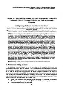
The combined effects of recruitment and mortality without grazing (i.e. grazing pressure p = 0) is a cubic equation, and the rate of change in the population initially declines before giving rise to the familiar hump-shaped curve usually associated with logistic growth (Fig. 4). The initial decline in recruitment is an Allee effect and is due to the low numbers of adults (Fig. 4a). There is no enhancement of recruitment without adults present, so the per capita rate of mortality at first outpaces the mass supply rate of recruits. The enhancement is a per capita effect, i.e. the more adults are present, the larger is the effect on the per individual recruitment rate, although the additional benefit declines with density and the curve saturates. The individual contributions of mortality, mass supply, and facilitation are non-linear, but none shows a threshold.

c

b

Species 2

194

Species 1

Species 2 isocline

Species 1

K1 > K2 > βK2 α

K1 > K2 > βK2 α

0

K1 = K2 α

K1 =

K2 β

Resource levels (K2 increases with resource levels) Fig. 3. Standard Lotka-Volterra model for 2-species competition showing hysteresis-like behavior with changes in resource levels expressed as changes in equilibrium density, K2. The 3 phase diagrams (a–c) show 0 isoclines for Species 1 and 2 at 3 points along the resource gradient. Below, the Z-shaped curve shows the equilibrium points for Species 2 (stable as solid line; breakpoint curve as dashed line). Solid lines give the stable equilibrium points (i.e. 0 and K2)

195

Petraitis & Hoffman: Thresholds and multiple states

0.35

Per capita rates

0.25 0.20 0.15

Deaths Recruitment Input of recruits Facilitation of recruitment

0.10 0.05 0.00

0

200

400

600

800

1000

1200

1400

Density 50

b 40

30

20

10

DISCUSSION

Unexploited Grazing 0

0

200

400

600

800

1000

1200

1400

Density 1400

Equilbrium density

Our critique suggests a single important lesson for ecologists, viz. demonstrations or observations of thresholds at 1 level provide little or no insight into thresholds at another. A threshold in a parameter does not necessarily mean there will be an abrupt shift between equilibrium states. We have shown in both linear and non-linear models how threshold behavior in state variables can occur without a threshold in parameters. The presence or lack of a threshold in one does not imply the presence or lack of a threshold in the other. The same is true for the relationship or lack thereof between transient behavior and parameters. Obviously there are many possibilities moving from observations of parameters to observations of equilibrium states and from equilibrium states to changes over time. The 8 curves in the 5 panels given in Fig. 1 alone provide 18 possible combinations, although not all are plausible. Yet, it is very difficult to use the plausible combinations to categorize the various studies reported in the literature, even though there have been numerous and well known efforts to catalogue examples of thresholds (May 1977, Scheffer et al. 2001, Folke et al. 2004, Knowlton 2004, Orth et al. 2006, Mumby 2009). The major obstacles to classification are inconsistent terminology, the potential for interactive effects between parameters and state variables, the use of models to confirm rather than to refute patterns, and the limits of inferences that can be drawn from

a

0.30

Rate of change

When grazing is added, the equilibrium density of the exploited species is a balance between the population’s rate of growth and the rate of grazing (Fig. 4b). As grazing pressure (p) increases, the system moves from 1 stable equilibrium point to 2 stable and 1 unstable points, and finally to back to 1 stable point. The transition from 1 stable point to 3 points is discontinuous and occurs over a very small change in p. The system has multiple stable states in the classic sense as defined by May (1977), even though none of the per capita rates shows step-like changes with changes in density. The range and relative impact of grazing are surprisingly small given the dramatic effect of grazing on the equilibrium density (Fig. 4c). Multiple stable states in this model occur only if p is between 0.0194 and 0.0467, which is between one-twelfth and one-fifth the per capita rate of mortality (i.e. v[N]). The range is extraordinarily narrow considering that p can lie between 0 and 1, although for p > 0.06, the equilibrium density drops below 10% of the density of an unexploited population.

c

1200 1000 800

Stable points Breakpoint curve

600 400 200

0.01

0.02

0.03

0.04

Grazing parameter ( p)

0.05

0.06

Fig. 4. Grazing model with multiple stable states. (a) Per capita rates for the supply of recruits, facilitation, and mortality as functions of density (N, where N = no. of adults per unit area). Per capita input of recruits equals s/N, where s = 25.7 recruits and is the max. no. of recruits. Per capita rates of facilitation and mortality are ƒ(N) = aN + bN 2 and v(N) = c + dN 2,where a = 3.8 × 10– 4, b = –1.4 × 10– 7, c = 0.162, and d = 6.0 × 10– 8. Parameters a, b, c and d are arbitrary and chosen to produce the shapes of the curves shown. (b) Population growth rate in the absence of grazing (solid line, unexploited) and the harvest rates under 3 levels of grazing (dashed lines). Solid (open) circles show stable (unstable) equilibrium points. (c) Equilibrium densities as a function of the rate of grazing. p is the intensity of grazing (i.e. the slope of the dashed line showing the level of grazing in panel b)

196

Mar Ecol Prog Ser 413: 189–200, 2010

experiments. We briefly discuss several modeling efforts and experimental studies of multiple stable states to illustrate these difficulties.

Terminology is inconsistent Different terms are used to describe the same concept and the same term is used for different concepts. The term ‘threshold’ itself has been applied not only to continuous step-like changes in parameters (Fig. 1a), equilibrium states (Fig. 1c), and transient states (Fig. 1e), but also to discontinuous changes in equilibrium states in response to small, continuous, and smooth changes in a parameter (Fig. 1d). The distinctions and relationships between parameters, equilibrium states, and transient behaviors are often unclear. Typically changes in parameters are conceptualized as changes over time and then linked to either changes in ecosystem status over time or in equilibrium state (Lake 2000, Andersen et al. 2009). For example, Lake (2000) noted that environmental conditions can change linearly over time (‘ramp disturbances’), and yet give rise to steep but smooth changes in the equilibrium state (‘press responses’). Andersen et al. (2009, their Fig. 1) covered much of the same ground as Lake (2000) but listed 3 classes of thresholds — driver thresholds, state thresholds, and driver–state hysteresis — that differ from Lake (2000) in meaning and confound the cause and effect relationship between parameters and state variables.

Interactive effects often blur the distinction between parameters and state variables In the perfect world of modeling, a perturbation of a state variable occurs without any effect on parameters. For example, in Fig. 1d the perturbation of the ecosystem state across the breakpoint curve is assumed to occur without changing the parameter space. The path of the perturbation does not affect the parameter space (i.e. the double-headed arrow in Fig. 1d, which is the perturbation of the state variable, runs parallel to the y-axis). In nature, a perturbation of an ecosystem engineer is likely to affect parameters such as recruitment, the per capita rate of predation, or the strength of competition, so it is very likely that a perturbation changes both the state variables and the parameters. This seems to be the case with seagrasses, which are well-known ecosystem engineers. Dramatic collapses of seagrass-dominated communities have been observed worldwide, owing to a suite of stressors including eutrophication, coastal loading of sediment and contaminants, rises in sea level and water temperature,

increased frequency and intensity of storms, expansion of aquaculture, and spread of non-native species (Orth et al. 2006). Recovery efforts are often unsuccessful (approximately 30% success rate, Orth et al. 2006), and models of multiple stable states have been developed to explain the apparent hysteresis between seagrass meadows and turbid algal states (van der Heide et al. 2007, Viaroli et al. 2008). In a similar model for Zostera marina, van der Heide et al. (2007) suggested that once Z. marina falls below a critical density threshold (i.e. crosses the breakpoint curve), turbidity prevents enough stems from recovering to restore ecosystem function. Z. marina reduces water movement and as a consequence, reduces turbidity. It is, thus, assumed that this ecosystem function controls light availability, which in turn has a positive feedback loop by promoting plant growth (Scheffer et al. 2001, van der Heide et al. 2007). The model includes a steep threshold, and not surprisingly, the equilibrium densities of Zmarina as a function of current velocity show a bifurcation and bistability. Yet there is a bit of circularity, since it is assumed that Z. marina density both affects and is a function of water movement. Viaroli et al. (2008) proposed a similar model to explain the occurrence of seagrass beds (Ruppia and Zostera spp.) and algal communities (Cladophora, Gracilaria, and Ulva spp.) in Mediterranean lagoons. Here the bifurcation is a function of nutrient loading. The system also has feedback loops, which increases the likelihood of thresholds in parameters. For example, high densities of seagrasses may be able to buffer moderate nitrogen loading through uptake and storage, which is followed by slow decomposition of seagrass detritus (Buchsbaum et al. 1991). This in turn controls algal growth and prevents high densities of macrophytes and phytoplankton that would otherwise reduce light penetration and inhibit seagrass growth. Viaroli et al. (2008) referred to the thresholds encompassing the parameter space where stable states are possible as ‘thresholds of reversibility’, beyond which any perturbation in state variables cannot flip the system to the alternative state (e.g. below T1 and above T2 in Fig. 1d). As in the case with seagrasses, it has been repeatedly suggested that thresholds and, thus, multiple stable states are associated with ecosystem engineers, environmental switches, and stressful abiotic conditions (Knowlton 1992, 2004, Wilson & Agnew 1992, Petraitis & Dudgeon 1999, Didham et al. 2005). However, all of these ecological features can be found in systems that contain neither thresholds nor multiple stable states, and thus the presence of ecosystem engineers and other environmental conditions does not guarantee the existence of thresholds or multiple stable states.

Petraitis & Hoffman: Thresholds and multiple states

Use of models to infer mechanism Observations of sudden shifts over time are commonly cited as examples of multiple stable states (e.g. Scheffer et al. 2001). The observation of a threshold over time is then modeled as a threshold in a parameter to produce a system with multiple stable states. It has even been suggested that the observation of rapid shifts between states is ‘[t]he key characteristic of a regime shift’ in systems with multiple stable states (deYoung et al. 2004, p. 145). In marine systems, the approach of moving from observation to confirmatory models has been commonly used in pelagic fisheries or oceanographic studies where the spatial scale precludes the possibility of undertaking manipulative experiments (Hare & Mantua 2000, Collie et al. 2004, deYoung et al. 2004, Mantua 2004, Andersen et al. 2009). This approach has also been used in studies of seagrass meadows, coral reefs, and pelagic fisheries, and the models almost always include a threshold in a parameter. The notion that there must be a link between thresholds at one level to thresholds in another is deeply embedded in all of these approaches. For example, Collie et al. (2004) used a model of multiple stable states to explain the collapse of George’s Bank haddock Melanogrammus aeglefinus. From the 1930s to 1950s, haddock stocks were consistently high (estimated to be 100 000 to 180 000 t, ‘haddock-rich’ state) despite a harvesting rate between 20 and 45% of estimated biomass. Haddock biomass spiked sharply to over 400 000 t in the early 1960s, followed by a rapid crash that is believed to be triggered by high rates of harvesting (Fogarty & Murawski 1998). Biomass wavered below 50 000 t for most of the remainder of the century (‘haddock-poor’ state), with a brief moderate recovery peaking at 100 000 t in 1980 and another recovery of similar magnitude leading up to the year 2000. With the exception of 3 years, harvesting rate during the haddock-poor period was less than or equal to mortality during the haddock-rich period (9 to 45%). Collie et al. (2004) developed a predator–prey model that exhibited hysteresis in equilibrium stock levels with 2 thresholds in harvesting rate. They found a rapid drop to the haddock-poor state at a harvesting rate of 36%, and a sharp transition to the haddock-rich state at a rate of 21%. This hysteresis is consistent with the notion that haddock dynamics contains a discontinuous regime shift between alternative stable states. Along the same lines, van Leeuwen et al. (2008) modeled the collapse of Baltic Sea cod Gadus morhua and also referred to 2 specific harvesting rates as thresholds. In the Baltic Sea, cod stocks and fishing pressure were high from 1974 to 1987. It is assumed that climate forcing from 1988 to 1993 led to decreases in salinity and oxygen, with concurrent increases in

197

temperature and nutrients. During this period, cod biomass plummeted despite no obvious change in harvesting rates. Abiotic conditions reversed to previous levels between 1994 and 2005, but cod biomass remained low (Möllmann et al. 2009). Van Leeuwen et al. (2008) proposed that high and low cod biomasses are alternative stable states that were controlled by adult cod predation on juvenile sprat Sprattus sprattus. They suggested that when present in sufficient numbers, adult cod exhibit top-down control of juvenile sprat, releasing the juveniles from intraspecific competition and promoting rapid maturation and reproduction. At low cod densities, juvenile sprat face strong intraspecific competition and remain in a young adult phase for a long period, where they are too large to be eaten by adult cod but not large enough to reproduce and promote recovery. The authors termed this scenario an ‘emergent Allee effect’ because it based on scarcity of adult cod. Similarly, Mumby et al. (2007) constructed a model of reef coral cover that exhibits a bifurcation as grazing intensity varies. Under strong grazing pressure, as in the Caribbean prior to mass mortality of the urchin Diadema antillarum, the system shows a single stable equilibrium of coral dominance. At low grazing pressure, the only stable equilibrium is macroalgae dominance. At intermediate grazing densities, there are 2 potential stable states – either coral or macroalgae dominance. Mumby et al. (2007) used the term ‘threshold’ in several ways. They referred to ‘critical thresholds of grazing and coral cover beyond which resilience is lost’ (Mumby et al. 2007, p. 98), and in a single phrase apply the term to both equilibrium states (i.e. coral cover) and parameter values (i.e. the rate of grazing) at which the bifurcations occur. Mumby (2009) also referred to specific values for the grazing parameter and the unstable equilibria (i.e. the breakpoint curve) as thresholds. Even so, development and use of models with multiple stable states and thresholds has strengths. Models can provide some of the most compelling examples of plausibility of multiple stable states. However, they are often difficult to confirm independently, and we suggest that modeling should include alternative scenarios that provide clear-cut and testable predictions. This is rarely the case. Experimental studies Misunderstanding about the lack of linkage between thresholds at one level versus another has also affected how ecologists have approached the detection of thresholds and multiple stable states experimentally. For example, in the western Pacific, abrupt temporal changes in mussel and macroalgal cover have been

198

Mar Ecol Prog Ser 413: 189–200, 2010

reported in response to experimental removal of seastars Pisaster ochraceus and to El Niño effects (Paine 1974, Paine et al. 1985, Paine & Trimble 2004). The changes are well documented and matched against control conditions. Paine & Trimble (2004) stated that the shift is evidence for multiple stable states, but it appears that the existence of hysteresis is inferred from the sudden shifts over time. Konar & Estes (2003) addressed abrupt spatial shifts in the boundary between kelps and barrens. They manipulated both kelps and urchins and provided good evidence that the presence of kelps keeps out urchins and thus sets the boundary. They suggested that the sharp boundary is the edge between 2 alternative stable states and implicitly assumed that the system was being pushed across the breakpoint curve through their manipulation of kelps and urchins, which are state variables. In the western Atlantic, Petraitis and colleagues have tested whether mussel beds and seaweed stands are alternative states and have explicitly examined the links from parameters to state variables to changes over time. They have experimentally shown sharp thresholds in barnacle and mussel recruitment and rates of predation on mussels and non-linear changes in fucoid recruitment with clearing size, which mimics the damage due to ice scour (Petraitis & Dudgeon 1999, Dudgeon & Petraitis 2001, Petraitis et al. 2003). They demonstrated that these effects translated into changes in adult densities and divergent successional patterns (Petraitis & Dudgeon 2005, Methratta & Petraitis 2008) and that some areas that were seaweed stands are now becoming mussel beds (Petraitis et al. 2009). There has been some discussion whether the thresholds in the mussel–seaweed system are an example of multiple states or 2 states under different levels of top-down control (Bertness et al. 2002, 2004, Petraitis & Dudgeon 2004a), although Petraitis et al. (2009) suggested how these 2 seemingly different views can be reconciled. These experimental studies document abrupt changes or thresholds in parameters or state variables and place those observations in the context of multiple stable states. Yet again, thresholds at one level are not proof of either thresholds at another level or the existence of multiple stable states. Indeed, multiple stable states can arise in systems in which parameters change in a linear fashion with changes in environmental conditions. Thus, demonstrations that ecosystems show abrupt shifts in parameters, species composition, or other state variables with small changes in environmental conditions are not sufficient tests for multiple stable states. There are ways to test for multiple states that do not depend on linking thresholds in parameters to thresholds in state

variables, and Petraitis & Dudgeon (2004b) discussed how experiments using Before-After, Control-Impact (BACI) designs could be used to test for multiple states. Our brief summary does not cover all that has been published on thresholds and multiple stable states in marine ecosystems and does not include the many studies that have been done in other systems. Many of the issues we have raised are well known and widely discussed in other areas of ecology (e.g. see Lake 2000, Huggett 2005, Bestelmeyer 2006, Groffman et al. 2006), and it is surprising to us how little cross-citation occurs among different disciplines. There is also the unsettling possibility that thresholds, while widely reported, are not the norm in ecological systems because negative results are rarely reported (Rosenthal 1979, Csada et al. 1996).

What is a threshold? Finally, it is useful to understand how the 2 conventional definitions of thresholds may color the observations made by ecologists. In the most conventional sense, a threshold is nothing more than the sill of a door or window. This functional architectural feature is used to delimit the inside and outside of a house and as an allusion for important milestones in life. The other definition comes from early developers of physiological psychology who viewed a threshold as the level of stimulus required to elicit a response. Fechner, who did pioneering work in experimental psychology in the mid 1800s and who introduced the concept of the median, strictly defined a threshold as the level of stimulus perceived by half of the subjects (e.g. Bi & Ennis 1998). For example, the auditory threshold for hearing for humans – the level of sound that 50% of humans can hear – is about 2 × 10– 5 Pa at 1000 Hz (approximately B5, which is the B in the second octave above middle C). Both definitions imply that small incremental changes in some condition or input have no or little effect until a defined limit is reached. At that point, the system enters a new state. These conventional definitions encompass the ecological notion of passing over the breakpoint curve or ridge separating 2 basins of attraction, but neither definition captures what ecologists usually mean when the term threshold is used to explain sudden shifts. The more important point is that both definitions rely on a limit that is set independently – the sill of the door or the median value. To the extent that ecologists fail to define thresholds independently of the processes under study, the current conceptualizations of thresholds in ecological systems may not be good metaphors for what happens in nature.

Petraitis & Hoffman: Thresholds and multiple states

Acknowledgements. This paper is dedicated to the memory of Larry Slobodkin for his wonderful insights that he so freely provided to so many graduate students. This work was supported by a National Science Foundation award to P.S.P. (DEB LTREB 03-14980).

➤ LITERATURE CITED

➤ Andersen T, Carstensen J, Hernandez-Garcia E, Duarte CM ➤ ➤ ➤ ➤ ➤

➤

➤ ➤ ➤ ➤ ➤ ➤ ➤ ➤

➤

➤ ➤

(2009) Ecological thresholds and regime shifts: approaches to identification. Trends Ecol Evol 24:49–57 Beisner BE, Haydon DT, Cuddington K (2003) Alternative stable states in ecology. Front Ecol Environ 1:376–382 Bender EA, Case TJ, Gilpin ME (1984) Perturbation experiments in community ecology — theory and practice. Ecology 65:1–13 Bertness MD, Trussell GC, Ewanchuk PJ, Silliman BR (2002) Do alternate stable community states exist in the Gulf of Maine rocky intertidal zone? Ecology 83:3434–3448 Bertness MD, Trussell GC, Ewanchuk PJ, Silliman BR (2004) Do alternate stable community states exist in the Gulf of Maine rocky intertidal zone? Reply. Ecology 85:1165–1167 Bestelmeyer BT (2006) Threshold concepts and their use in rangeland management and restoration: the good, the bad, and the insidious. Restor Ecol 14:325–329 Bi J, Ennis DM (1998) Sensory thresholds: concepts and methods. J Sensory Studies 13:133–148 Buchsbaum R, Valiela I, Swain T, Dzierzeski M, Allen S (1991) Available and refractory nitrogen in detritus of coastal vascular plants and macroalgae. Mar Ecol Prog Ser 72: 131–143 Collie JS, Richardson K, Steele JH (2004) Regime shifts: Can ecological theory illuminate the mechanisms? Prog Oceanogr 60:281–302 Connell JH, Sousa WP (1983) On the evidence needed to judge ecological stability or persistence. Am Nat 121: 789–824 Csada RD, James PC, Espie RHM (1996) The ‘file drawer problem’ of non-significant results: Does it apply to biological research? Oikos 76:591–593 deYoung B, Harris R, Alheit J, Beaugrand G, Mantua N, Shannon L (2004) Detecting regime shifts in the ocean: data considerations. Prog Oceanogr 60:143–164 Didham RK, Watts CH, Norton DA (2005) Are systems with strong underlying abiotic regimes more likely to exhibit alternative stable states? Oikos 110:409–416 Doak DF, Estes JA, Halpern BS, Jacob U and others (2008) Understanding and predicting ecological dynamics: Are major surprises inevitable? Ecology 89:952–961 Done TJ (1992) Phase-shifts in coral-reef communities and their ecological significance. Hydrobiologia 247:121–132 Dudgeon S, Petraitis PS (2001) Scale-dependent recruitment and divergence of intertidal communities. Ecology 82: 991–1006 Fogarty MJ, Murawski SA (1998) Large-scale disturbance and the structure of marine system: fishery impacts on Georges Bank. Ecol Appl 8:S6–S22 Folke C, Carpenter S, Walker B, Scheffer M, Elmqvist T, Gunderson L, Holling CS (2004) Regime shifts, resilience, and biodiversity in ecosystem management. Annu Rev Ecol Evol Syst 35:557–581 Frank PW (1968) Life histories and community stability. Ecology 49:355–357 Groffman P, Baron J, Blett T, Gold A and others (2006) Ecological thresholds: the key to successful environmental management or an important concept with no practical

application? Ecosystems 9:1–13 SR, Mantua NJ (2000) Empirical evidence for North Pacific regime shifts in 1977 and 1989. Prog Oceanogr 47:103–145 Hastings A (2004) Transients: the key to long-term ecological understanding? Trends Ecol Evol 19:39–45 Huggett AJ (2005) The concept and utility of ‘ecological thresholds’ in biodiversity conservation. Biol Conserv 124: 301–310 Knowlton N (1992) Thresholds and multiple stable states in coral-reef community dynamics. Am Zool 32:674–682 Knowlton N (2004) Multiple ‘stable’ states and the conservation of marine ecosystems. Prog Oceanogr 60:387–396 Konar B, Estes JA (2003) The stability of boundary regions between kelp beds and deforested areas. Ecology 84:174–185 Lake PS (2000) Disturbance, patchiness, and diversity in streams. J N Am Benthol Soc 19:573–592 Lewontin RC (1969) The meaning of stability. In: Woodwell GM, Smith HH (eds) Diversity and stability in ecological systems. Brookhaven Symp Biol 22:13–24 Lotka AJ (1956) Elements of mathematical biology. Dover Publications, New York, NY Mantua N (2004) Methods for detecting regime shifts in large marine ecosystems: a review with approaches applied to North Pacific data. Prog Oceanogr 60:165–182 May RM (1977) Thresholds and breakpoints in ecosystems with a multiplicity of stable states. Nature 269:471–477 Methratta ET, Petraitis PS (2008) Propagation of scale-dependent effects from recruits to adults in barnacles and seaweeds. Ecology 89:3128–3137 Möllmann C, Diekmann R, Muller-Karulis B, Kornilovs G, Plikshs M, Axe P (2009) Reorganization of a large marine ecosystem due to atmospheric and anthropogenic pressure: a discontinuous regime shift in the Central Baltic Sea. Glob Change Biol 15:1377–1393 Mumby PJ (2009) Phase shifts and the stability of macroalgal communities on Caribbean coral reefs. Coral Reefs 28: 761–773 Mumby PJ, Hastings A, Edwards HJ (2007) Thresholds and the resilience of Caribbean coral reefs. Nature 450:98–101 Noy-Meir I (1975) Stability of grazing systems: an application of predator–prey graphs. J Ecol 63:459–481 Orth RJ, Carruthers TJB, Dennison WC, Duarte CM and others (2006) A global crisis for seagrass ecosystems. Bioscience 56:987–996 Paine RT (1974) Intertidal community structure — experimental studies on relationship between a dominant competitor and its principal predator. Oecologia 15:93–120 Paine RT, Trimble AC (2004) Abrupt community change on a rocky shore — biological mechanisms contributing to the potential formation of an alternative state. Ecol Lett 7: 441–445 Paine RT, Castilla JC, Cancino J (1985) Perturbation and recovery patterns of starfish-dominated intertidal assemblages in Chile, New Zealand, and Washington State. Am Nat 125:679–691 Petraitis PS, Dudgeon SR (1999) Experimental evidence for the origin of alternative communities on rocky intertidal shores. Oikos 84:239–245 Petraitis PS, Dudgeon SR (2004a) Detection of alternative stable states in marine communities. J Exp Mar Biol Ecol 300: 343–371 Petraitis PS, Dudgeon SR (2004b) Do alternate stable community states exist in the Gulf of Maine rocky intertidal zone? Comment. Ecology 85:1160–1165 Petraitis PS, Dudgeon SR (2005) Divergent succession and

➤ Hare ➤

➤ ➤ ➤

➤ ➤ ➤ ➤

➤ ➤ ➤ ➤ ➤ ➤

➤

➤

➤ ➤

➤

199

200

➤ ➤

➤ ➤ ➤ ➤

Mar Ecol Prog Ser 413: 189–200, 2010

implications for alternative states on rocky intertidal shores. J Exp Mar Biol Ecol 326:14–26 Petraitis PS, Latham RE (1999) The importance of scale in testing the origins of alternative community states. Ecology 80:429–442 Petraitis PS, Rhile EC, Dudgeon S (2003) Survivorship of juvenile barnacles and mussels: spatial dependence and the origin of alternative communities. J Exp Mar Biol Ecol 293:217–236 Petraitis PS, Methratta ET, Rhile EC, Vidargas NA, Dudgeon SR (2009) Experimental confirmation of multiple community states in a marine ecosystem. Oecologia 161:139–148 Rosenthal R (1979) The file drawer problem and tolerance for null results. Psychol Bull 86:638–641 Scheffer MS, Hosper H, Meijer ML, Moss B, Jeppesen E (1993) Alternative equilibria in shallow lakes. Trends Ecol Evol 8:275–279 Scheffer M, Carpenter S, Foley JA, Folke C, Walker B (2001) Catastrophic shifts in ecosystems. Nature 413:591–596 Schröder A, Persson L, De Roos AM (2005) Direct experimental evidence for alternative stable states: a review. Oikos 110:3–19 Submitted: November 4, 2009; Accepted: June 3, 2010

➤ ➤

➤

➤

Slobodkin LB (1961) Growth and regulation of animal populations. Holt, Rinehart and Winston, New York, NY Suding KN, Hobbs RJ (2009) Threshold models in restoration and conservation: a developing framework. Trends Ecol Evol 24:271–279 Thrush SF, Hewitt JE, Dayton PK, Coco G, Lohrer AM, Norkko A, Norkko J, Chiantore M (2009) Forecasting the limits of resilience: integrating empirical research with theory. Proc Biol Sci 276:3209–3217 van der Heide T, van Nes EH, Geerling GW, Smolders AJP, Bouma TJ, van Katwijk MM (2007) Positive feedbacks in seagrass ecosystems: implications for success in conservation and restoration. Ecosystems 10:1311–1322 van Leeuwen A, De Roos AM, Persson L (2008) How cod shapes its world. J Sea Res 60:89–104 Viaroli P, Bartoli M, Giordani G, Naldi M, Orfanidis S, Zaldivar JM (2008) Community shifts, alternative stable states, biogeochemical controls and feedbacks in eutrophic coastal lagoons: a brief overview. Aquat Conserv Mar Freshw Ecosyst 18:S105–S117 Wilson JB, Agnew ADQ (1992) Positive-feedback switches in plant communities. Adv Ecol Res 23:264–336 Proofs received from author(s): August 10, 2010