Multiple View Based 3D Object Classification Using Ensemble Learning of Local Subspaces Jianing Wu, Kazuhiro Fukui Graduate school of Systems and Information Engineering, University of Tsukuba
[email protected],
[email protected] Abstract Multiple observation improves the performance of 3D object classification. However, since the distribution of feature vectors obtained from multiple view points have strong nonlinear structure, the kernel-based methods are often introduced with nonlinear mapping. By mapping feature vectors to a higher dimensional space, kernel-based methods transform the distribution to weaken its nonlinearity. Although they have been succeeded in many applications, their computation cost is large. Therefore we aim to construct a comparable method with the kernel-based methods without using nonlinear mapping. Firstly we attempt to approximate a distribution of feature vectors with multiple local subspaces. Secondly we combine local subspace approximation with ensemble learning algorithm to form a new classifier. We will demonstrate that our method can achieve comparable performance with kernel methods through evaluation experiments using multiple view images of 3D objects from a public data set.
1. Introduction This paper proposes a view-based method for classifying 3D object which can achieve comparable performance with kernel-based method without using nonlinear mapping. Among various view-based object classification methods that have been proposed, Mutual Subspace Method (MSM)[1] has been applied for face and object recognition and was shown to be one of the most efficient methods for object recognition. In view-based object classification, an n×n image pattern is represented as a feature vector in n×n-dimensional vector space. MSM generates a class subspace by applying principal component analysis (PCA) in learning phase. This is done from the distribution of feature vectors belong to each class. In classification phase, an input subspace is generated from multiple input feature vectors by PCA. The canonical angles[7] between the input subspace and
978-1-4244-2175-6/08/$25.00 ©2008 IEEE
class subspaces are then calculated. Finally, the end results is the class label of the subspace which has smallest canonical angle. In general the distribution of feature vectors obtained from multiple view points has strong nonlinear structure. MSM therefore does not work well in classifying multiple view distribution, because such a distribution cannot be represented by a linear subspace without any overlap. To solve this problem, MSM has been extended to a nonlinear method called Kernel Mutual Subspace Method (KMSM) [2][3] by introducing nonlinear mapping with a kernel function. KMSM has improved the performance of MSM largely. However KMSM consumes more computation time compared to MSM. KMSM follows an N 2 order, as a result the above problem becomes more serious when the number of feature vectors and classes of the object is larger. Also KMSM has a difficult problem of parameter selection of the kernel function. Since these parameters are difficult to be determined theoretically, while the performance depends extremely on the characteristic of these parameters. For the above reasons, we aim to achieve comparable performance with KMSM for the classification of nonlinearly distributed feature vectors without using nonlinear mapping. Our key idea is that we approximate a distribution of feature vectors with multiple local subspaces instead of a single subspace as in MSM. This operation weakens the nonlinearity in each local subspace as shown in Fig.1. However, it is difficult to optimize the number of local subspaces and the dimension of each local subspace, we generate multiple sets of local subspaces by changing these parameters. Then ensemble learning is applied with the above local subspaces. The rest of this paper is organized as follows: In Section 2, the detail of the proposed method is presented. Section 3 outlines the process of classification. In Section 4 we evaluate the proposed method through classi-
Distribution of feature vectors
A subspace
Dimension i of local subspaces
A set of local subspaces
Figure 1. Comparison between approximation using a linear subspace and a set of local subspaces .
fication experiments. Finally in Section 5, the conclusion is made.
2. The proposed method 2.1
Definition of local subspace
To realize our idea, we apply k-means method to the distribution to obtain k sub sets. We then apply PCA to each sub set, to obtain basis vectors of a subspace as shown in Fig.1. The basis vectors of each subspace are calculated as the eigenvectors corresponding to the larger eigenvalues of autocorrelation matrix. We call these subspaces as local subspaces.
2.2 Definition of similarity based on sets of local subspaces Let an input subspace be A, a set of local subspaces belong to class c be Bc , the j-th local subspace belongs to Bc be Bcj . We assume the dimension of A be M , the dimension of Bcj be N , for convenience N ≤ M . The similarity between A and Bcj is defined by using the canonical angle θ between these two subspaces as follows[1]. Ang(A, Bcj ) =
cos2 θ
(1) |(u, v)| ||u||2 ||v||2 2
=
max
u∈A,v∈Bc j
, (2)
||u||̸=0,||v||̸=0
where cos2 θ is calculated as the largest eigenvalue of the following matrix. X xmn
= =
(xmn ) N ∑
(3)
m, n = 1...M
(ψm , ϕl )(ϕl , ψn)
,
(4)
l=1
where ψm and ϕl are the m-th and the l-th basis vector of subspace A and Bcj , (ψm , ϕl ) represents the inner product of ψm and ϕl .
Number k of clusters to generate local subspaces Local subspace Original distribution of feature vectors Figure 2. The relation between the number of clusters and the dimension of the local subspaces.
The similarity of A and Bc is calculated from the following equation. Simweak (A, Bc ) =
k ∑
Ang(A, Bcj ) .
(5)
j=1
2.3
Ensemble learning
Classification performance changes in relation to the dimensions of the local subspaces and the number of clusters (k in k-means method). Thus, to achieve the best classification performance, we need to optimize these parameters. However, since we have many possible combinations of these parameters as shown in Fig.2, it is difficult to select the most optimum one from them theoretically. To overcome this problem we consider a classifier using each set of local subspaces, and apply ensemble learning to these classifiers. By changing the dimension i of local and input subspaces and the number k of cluster to generate local subspace, multiple weak classifiers are obtained. We combine their similarities to obtain the final similarity as follows. ∑∑ Sim(A, Bc ) = Simweak (A, Bc ) (6) i
2.4
k
Adjusting weights of local subspaces
Although each set of local subspaces represents the distribution of the training patterns well, there is no reason to assume a priori that it is the optimal set of local subspaces in terms of classification performance. We
A Sim(A, B1 ), Sim(A, B2 ), . . . , Sim(A, BL )
B11 B12 B13
B21 B22 B23
BL 1 BL 2 BL 3
Figure 4. Flow chart of the classification phase. B11 B12 B13
B21 B22 B23
BL 1 BL 2 BL 3
In classification phase, The similarity of an input subspace A with each local subspace Bcj is calculated by using Equation (5) and then combine these similarities following Equation (6). The class that has highest similarity is the result of the classification.
Figure 3. Flow chart of the learning phase.
4. Experiments therefore introduce a weight to each local subspace, considering the relation with rival class sets of local subspaces. To introduce weights, we rewrite Equation (5) as follows. Simweak (A, Bc ) =
k ∑
αjc Ang(A, Bcj )
,
(7)
j=1
where αjc is the weight of the local subspace Bcj . The weights are obtained by preliminary classification experiments using training data as follows. 1. Initialize: αjc = 1 2. Do for t = 1, ..., N , (N is the number of learning data) Record the number of classification error EBcj for each Bcj 3 Calculate the training error rate εBcj as EBcj /N 4 Calculate weight: αjc ← 1 − εBcj 5. Normalize weight
3. Flow of classification process The process of the proposed method consists of learning phase as shown in Fig.3 and classification phase as shown in Fig.4. We outline the process of the proposed method, considering the case with L classes as an example. In learning phase, we use a set of local subspaces to approximate the distribution of each class. Multiple sets of these local subspaces are generated with changing the number of clusters and dimension of local subspaces. The weight of each local subspace is adjusted after local subspace generation.
We use a public data set ’The ETH-80 Image Set[8]’ to evaluate the proposed method. The data set has been created from 8 classes, 10 objects for each class. There are images taken from 41 different view points for each object. 5 objects are randomly choosed from the data set for each class for evaluation experiment. In learning phase 4 objects, 164 images per class are used for training. In classification phase 10 images (view points) of an untrained object are used as test input. By changing input and training data, classification experiment is repeated 1640 times for each method. The contribution rate for the dimension selection is set to 98%. The number of clusters for distribution division is set from 2 to 5. Firstly we compare the performance of the proposed method with MSM and KMSM. Secondly we compare the result of each weak classifier and the ensemble learned result, to demonstrate the contribution of ensemble learning to the classification performance. Thirdly we compare the performance of the proposed method before weighting (I) and after weighting (II). The weight of the proposed method is trained from learning data (trained for 800 times). Separability is an indicator normalized to 1.0, higher is better. EER (Equal Error Rate) is the intersection point of FAR (False Acceptance Rate) and FRR (False Reject Rate) curves, lower is better. The performance of MSM, the proposed method before weighting (I), and KMSM are shown in Table 1. The proposed method achieved a 17% advancement in classification performance compared to MSM. At the
Table 3. Result of weak classifiers. Cluster number Accuracy Sep. EER(%) rate(%) 2 73.0 0.41 14 3 77.5 0.40 15 4 75.3 0.41 17 5 72.0 0.40 15 Proposed method I 86.5 0.44 14
Figure 5. The ETH-80 Image Set. Table 1. Result of each method. Method Accuracy Sep. EER(%) rate(%) MSM 69.5 0.34 20 KMSM 87.2 0.41 15 Proposed method I 86.5 0.44 14 Proposed method II 94.7 0.55 9
same time the proposed method also achieved comparable performance with KMSM. In Table 2, we show the calculation time of each method in classification phase, which proved the computation complexity of the proposed method is far less than KMSM. We show the performance of each weak classifier in Table 3. It is shown that classification performance of the proposed method is higher than any of its weak classifier. Finally as shown in Table 1, the proposed method after weighting (II) further improved classification performance by 8% compared to the proposed method before weighting (I).
5. Conclusion We proposed a 3D object classification method using multiple view points. We approximate a distribution of feature vector with strong nonlinear structures by multiple local subspaces. We change number and dimen-
Table 2. Calculation time per input of each method. Method Time (second) MSM 0.1 Proposed method (I,II) 0.4 KMSM 3.1
sion of local subspaces and generate local subspaces at each combination. By applying ensemble learning to these local subspaces, the proposed method improved performance compared to MSM. The experimental results demonstrated that our method can achieve comparable performance with KMSM.
References [1] O. Yamaguchi, K. Fukui, K. Maeda: Face recognition using temporal image sequence. Proc. IEEE Third International Conference on Automatic Face and Gesture Recognition, pp.318-323, 1998. [2] H. Sakano, N. Mukawa: Kernel mutual subspace method for robust facial image recognition. Proc. Fourth International Conference on KnowledgeBased Intelligent Engineering Systems and Allied Technologies, Vol.1, pp.245-248, 2000. [3] L. Wolf, A. Shashua: Learning over sets using kernel principal angles. Journal of Machine Learning Research, Vol.4, pp.913-931, 2003. [4] Y. Freund: Boosting a weak learning algorithm by majority. Information and Computation, Vol.121, pp.256-285, 1995. [5] Y. Freund, R. E. Schapire: A decision-theoretic generalization of on-line learning and an application to boosting. Journal of Computer and System Sciences, No.55, pp.119-139, 1997 [6] B. Sch¨ olkopf, A. Smola, K. R. M¨ uller: Nonlinear principal component analysis as a kernel eigenvalue problem. Neural Computation, Vol.10, pp.12991319, 1998. [7] F. Chatelin: Eigenvalues of matrices. John Wiley& Sons, Chichester, 1993. [8] B. Leibe, B. Schiele: Analyzing appearance and contour based methods for object categorization. CVPR’03, Vol.2, pp.409-415 2003.