Author manuscript, published in "Signal Processing 83 (2003) 1487-1503" DOI : 10.1016/S0165-1684(03)00064-1
Multiscale estimation of vector field anisotropy Application to texture characterization
C. Germain, J.P. Da Costa, O. Lavialle, P. Baylou
AUTHOR’S AFFILIATION Christian Germain, Jean-Pierre Da Costa and Olivier Lavialle ENITA de Bordeaux
hal-00160721, version 1 - 7 Jul 2007
and Equipe Signal et Image, LAP UMR 5131, ENSEIRB. BP 201, 33175 Gradignan cedex – France. Email:
[email protected] –
[email protected] –
[email protected] Pierre Baylou Equipe Signal et Image, LAP UMR 5131, ENSEIRB – GDR-PRC ISIS. BP 99, 33402 Talence Cedex - France. Email:
[email protected]
KEYWORDS Image processing, texture, orientation field, anisotropy, observation scale.
1
ABSTRACT This paper deals with the characterization of the anisotropy of textured images. It is well known that either the dominant direction or the texture anisotropy strongly depends on the scale used for the observation. In this paper we propose a new operator for the estimation of the dominant direction, the Directional Mean Vector (DMV), which can be computed at any observation scale. Then, we present a new indicator for the estimation of the DMV field anisotropy. This indicator, called I so , is computed at a given observation scale. I so is based on the computation of the DMV field local differences. It is shown that the evolution of I so
hal-00160721, version 1 - 7 Jul 2007
versus the observation scale gives a curve which simultaneously characterizes the anisotropy of the texture and the size of the textural patterns. In order to establish this property, we build a specific texture model which allows to assess an analytical expression for I so . Finally, I so is applied to the characterization of various images including synthetic textures, Brodatz textures and composite material images. RESUME Ce manuscrit traite de la caractérisation de l'anisotropie des images texturées. Il est avéré que l'orientation dominante et l'anisotropie dépendent fortement de l'échelle d'observation. Nous proposons ici un nouvel opérateur pour l'estimation de la direction dominante: le Vecteur Directionnel Moyen (DMV) qui peut se calculer à des échelles variées. Ensuite, nous présentons un nouvel indicateur qui permet l'estimation de l'anisotropie du champ des DMV. Cet indicateur, nommé I so , est calculé à une échelle d'observation donnée. Il se fonde sur les différences locales du champ des DMV. Nous montrons que l'évolution de I so en fonction de l'échelle d'observation fournit une courbe qui caractérise à la fois l'anisotropie de la texture et la taille des motifs texturaux. Afin d'établir ce comportement, nous construisons un modèle textural et nous proposons, sur ce modèle, une expression analytique de la valeur d' I so . Enfin, I so est appliqué à la caractérisation de plusieurs types d'images et notamment de textures de Brodatz et d'images de matériaux composites.
2
1. INTRODUCTION As many natural pictures involve textured regions, the identification of relevant textural features has been widely addressed within the scope of either human perception [25] or image processing [10][21][33]. In [20], Haralick defines the tone-texture concept as a two-layered structure. The first layer specifies the local properties (i.e. tonal primitives) of texture and the second layer deals with the spatial interrelationships between the tonal primitives. In order to describe this two-level structure, either structural or statistical approaches have been proposed [20].
hal-00160721, version 1 - 7 Jul 2007
Structural approaches are based on the estimation of the parameters which drive the spatial arrangement of textural primitives. These primitives and their spatial arrangements are assumed to obey explicit or unknown stochastic laws. In statistical approaches, the tonal primitive the most frequently used is the image gray level. For example, the gray level based textural features are computed on spatial statistics derived from cooccurrence matrices [21][20][18] or interaction maps [8][9], or on parameters of stochastic texture models, such as Markov Random Fields [10]. As texture deals with the spatial arrangement of the gray levels, textural features will often describe geometric properties such as roughness, symmetry or directionality [33]. These features can therefore be used to describe physical properties of the observed objects. In [25], Julesz and Bergen identify the features, which they call textons, involved in preattentive vision. Rao and Lohse [33] try to identify the most relevant high level features required in the attentive inspection of images. In both approaches anisotropy appears to be an obvious feature for texture description. In this paper we consider directional textures, i.e. textures which consist, at least partially, of directional patterns, and we focus on anisotropy. Let us define the anisotropy as the existence
3
of a unique dominant orientation in the texture. The more the orientation is dominant, the more the texture is said anisotropic. The notion of anisotropy has been addressed in various papers [22][31] and has proved to be useful in practical tasks such as the detection of singular points in seismic pictures [14] or on finger tips [24], and the characterization of materials [17]. However, this definition differs from others (e.g. [9]) in the sense that the uniqueness of the dominant orientation plays a crucial part in the determination of the anisotropy. For instance, the anisotropy of a texture being a checkerboard of two definite orientations will decrease from strictly anisotropic when
hal-00160721, version 1 - 7 Jul 2007
the directions are equal, to non anisotropic when the directions are orthogonal. It should be noted that the non anisotropic case differs from the strictly isotropic case where the orientations are uniformly distributed. Another feature of both anisotropy and orientation is their strong dependence on the
Fig.1 observation scale, as it is shown in Figure 1 for a sinusoidal textured picture. At a small scale, as in windows #1, the dominant orientation may be very different from one window to the next. Thus, the texture appears to be poorly anisotropic. At a larger scale, as in windows #2, the dominant orientation is the same for the entire picture. The texture appears to be much more anisotropic. This example illustrates the need to associate anisotropy measurements with the scale at which the texture is observed. The observation scale can be seen, in fact, as a generalization of the notions of micro-texture and macro-texture, reported in previous works [1] on texture characterization. Indeed, a twolevel structure is often inadequate to describe natural textures which exhibit a continuous evolution of anisotropy as a function of scale. Several approaches have been proposed to provide an estimation of texture anisotropy. For example, spectral analysis tools are frequently used for this purpose. Anisotropy can be estimated from the power spectrum density in the Fourier domain. However, as this
4
estimation is usually performed on the entire picture, it is only valid at large scales. Gabor filters [5] deal efficiently with such a limitation, as they compute textural components for various scales and orientations. Thus, at a given scale, the variation of those components versus the orientation of the filter describes the anisotropy of the texture. Chetverikov et al. [8] proposed another approach based on the so-called Extended Grey Level Difference Histogram (EGLDH). For a given displacement, the evolution of the EGLDH feature versus the orientation is described by a curve called anisotropy indicatrix. The average curve for a range of displacements (e.g. short range and long range) can be used to determine
hal-00160721, version 1 - 7 Jul 2007
the dominant orientation when it exists. However, this estimation only takes into account the displacement between pixels. On the contrary, the approach we propose in this paper uses a definition of the observation scale which involves both the distance between the domains on which the orientation is estimated, and the area of these domains. The textural spectrum, introduced by He et al. [22] is based on the computation of a local texture descriptor. Textural features can be extracted from this spectrum. Among these features, the Degree of Direction, computed on a window of a given size, can be used for estimating anisotropy at various scales. However, this method can only take into account the directions defined by 0°, 45°, 90° and 135° angles, and leads to inaccurate estimations. Other authors address the problem of anisotropy by computing descriptors of the local gradient field [4][32][34][26][30]. Bigün [4] has shown that seeking anisotropy through a principal component analysis of the local power spectrum density is equivalent to analyzing the local gradient field. We propose in this paper a new orientation-based technique for anisotropy estimation. This approach consists of two main steps. Firstly, we estimate the orientation field at a given scale, based on the local gradient field. Secondly, we compute a scattering indicator for the orientations obtained at the previous stage. Both steps are iterated for various observation
5
scales. The set of the scattering measures forms an anisotropy curve which describes the anisotropy behavior versus the observation scale. The paper is organized as follows. In section 2, we introduce the Directional Mean Vector (DMV), an orientation estimator computed at a given scale n. In the third section, we define I so , an indicator for anisotropy measurement. In the fourth section we describe a specific model for textures which takes into account textural primitives of different sizes. The theoretical behavior of the anisotropy indicator I so is then studied using this model. The results are compared to simulation curves obtained on synthetic textures. Finally, in the fifth
hal-00160721, version 1 - 7 Jul 2007
section, this approach is applied to real textures taken from Brodatz’s album [6] and from composite material images.
2. ESTIMATION
OF THE MAIN DIRECTION OF A TEXTURE USING THE
DIRECTIONAL MEAN
VECTOR This step aims at the construction of a vector field describing the dominant orientations at a given observation scale. The estimation of a directional trend is achieved by Bigün et al. [3][4] and later by Kass and Witkin [26] and Rao [31][34], who propose a formulation for the local dominant orientation based on the gradient estimation. The approach proposed by Bigün et al. [3][4], is based on the local Fourier transform. It consists, through a Principal Component Analysis, in looking for the axis of maximum inertia of the local power spectrum. Using the Parseval theorem, this frequential approach can be expressed as an eigenvalue decomposition of the covariance matrix of the local gradient field. In order to take into account the axial nature of orientations, the formulation proposed by Kass and Witkin [26] and Rao [31][34] uses complex representations of the gradients. Through a variance-based criterion minimization, they prove that the optimal estimation of the dominant orientation is given by the argument of the sum of the squared gradient vectors. 6
This technique turns out to be equivalent to the approaches based on local Fourier transforms, such as [3][4]. Indeed, the square gradient formulation is simply a generalization of the double argument technique, which was first proposed by Mardia [28] and later by Baschelet [2], in the fields of statistics and biology. This technique is described below. In order to ensure noise robustness, several authors use smoothed gradients. For example, Kass and Witkin [26] apply a DoG (Difference of Gaussians) filter before deriving a finite difference gradient, while Rao [31][34] uses a simple Gaussian filter. In the context of edge detection, Canny [7] and Deriche [12][13] propose optimal gradient filters, also based on the
hal-00160721, version 1 - 7 Jul 2007
derivatives of a Gaussian. In order to consider both macrotextures and microtextures [1] with textural patterns barely a few pixels wide, we need a gradient estimator which is as local as possible. Indeed, using a smooth filter would not be adapted to such thin textural patterns. Moreover, fitting a DoG or a Gaussian filter to the size of micro-textural patterns would lead to a very small filter mask. This would turn out to be noise sensitive and finally, would be equivalent to using finite small size filters. Sobel's operator [23] appears to offer a good compromise between noise robustness and mask size. For this reason we use Sobel's gradient, except in cases where noise robustness and orientation accuracy are crucial. Sobel’s operator provides a vector field describing texture orientation at a local scale. Then, from this vector field, we have to estimate the directional trend of the texture at any scale, which is, in fact, a kind of average orientation. Note that the arithmetic mean cannot be used for estimating the mathematical expectation of the arguments of the gradients because in this case, arguments are periodic data [28]. Moreover, although the vector arguments are defined modulo 2π, we deal with orientations which must be considered modulo π. Indeed, two opposite vectors indicate the same orientation, but the arithmetic mean of their argument will
7
Fig.2
produce an orientation orthogonal to the desired vector orientation. Here, we compute an appropriate mean orientation derived from directional statistics, as defined in [28]. Definition 1 G Let {θ i } i =1 to m be the set of arguments of the vectors {vi }i =1 to m considered modulo π. The G arguments are chosen in [0, π[. Let {v i '} i=1 to m be the corresponding unit vectors with argument 2 × θ i . In this case, the mean direction θ of the set {θi } i =1 to m is defined by 1 ⎛ m G' ⎞ 1 ⎛ m ⎞ arg⎜ ∑ vi ⎟ or θ = arg⎜ ∑ e j 2θ i ⎟ in complex notation (j2=-1). (1) 2 ⎝ i =1 ⎠ 2 ⎝ i =1 ⎠ m G G It should be noted that θ is not defined if ∑ v i' = 0 . This singular case occurs when there is
θ=
i =1
hal-00160721, version 1 - 7 Jul 2007
no unique dominant orientation as discussed in section 1. Let us complete this definition in order to take into account the modulus of each gradient vector. This modulus gives information on the confidence associated with the orientation. Definition 2 Let z = re jθ be a realization of the complex random variable Z = Re jΘ , with both R and
Θ real random variables, Θ considered modulo π. The Directional Mean Vector (DMV) associated with the variable Z is given by the complex number
zM
Z2 = DMV ( Z ) = Z
1/ 2
⋅
Z2 Z
1/ 2
(2)
where ⋅ is the mathematical expectation. The argument of the DMV is an estimation of the dominant orientation of the vector set. Moreover, as shown in [28], the modulus of the DMV reflects the confidence we have in the orientation estimates. In practice, a field of DMVs is computed in the following way. At observation scale n, an N × N image is divided into windows of size n × n , producing a pavement of (N/n)² windows.
In each window, the DMV is computed using eq. (2). The robustness of the DMV is illustrated with a synthetic texture oriented at 80° (Fig. 2). White noise is added to this picture to provide a 0dB SNR. The DMV field is computed for 8
scales ranging from n=1 to n=32. Fig. 2c shows that the orientations of elementary vectors (scale n=1) are strongly affected by the noise. Only 80% of the arguments are in the range [27°, 134°]. Using the DMV at scale n=8 and n=32 , this interval is reduced to [74°, 86°] and [79°, 81°] respectively. These experiments show that the noise robustness of the DMV operator improves as the observation scale increases.
3. ESTIMATION OF THE ANISOTROPY OF A VECTOR FIELD Let now discuss some methods for measuring the scattering of the DMV field. The complex moment approach [5] gives the directions of symmetry of a texture as well as a magnitude
hal-00160721, version 1 - 7 Jul 2007
reflecting the scattering around these directions. Other approaches based on angular statistics provide indicators for the scattering of an orientation. Mardia showed in [28] that the modulus of the resulting vector proposed in equation (1) is sensitive to this scattering. Thereafter, he defined a circular variance S 0 based on the modulus of the vectors: G
S0
∑ v' = 1− G ∑ v'
i
i
0 ≤ S0 ≤ 1 .
,
(3)
i
i
A circular standard deviation s0 has also been proposed. ln(1 − S 0 ) , 0 ≤ s0 ≤ ∞ . (4) 2 Other indicators, reported in [28], [15] and [19], measure the scattering around the circular s0 = −
mean for the whole field. They are based on first order statistics only and do not take into account the fact that the same angular difference between two vectors will have different meanings depending on whether the vectors are close or far. Dealing with second order statistics, Davis et al. [11] proposed a generalization of the cooccurrence matrices based on the orientations of edges. Later, Kovalev et al. [27] also addressed orientation second-order statistics by deriving variograms from the texture orientation field. However, these second-
9
order approaches do not deal with the scale of analysis which plays a crucial role in estimating the orientation. Clearly, the angular difference between two vectors must be associated with the distance separating the corresponding windows. For this reason we propose a new scattering indicator, called I so , based on second order statistics. It computes the argument differences between neighboring vectors. These differences are weighted by the vector moduli in order to take into account the confidence we have in the orientation measurements. Definition 3 →
→
hal-00160721, version 1 - 7 Jul 2007
Consider the vector field { G s1 ... G sn } from which we want to estimate the anisotropy. These vectors are located on a 2-D lattice of sites { s1 ... sn }. Let C i , j be the clique →
→
composed of the neighboring vectors ( Gi , G j ) in the 4-neighborhood sense. Examples of horizontal and vertical cliques at small and large scales are given in Fig. 1. The proposed I so indicator is then defined by ⎡
I so =
(
→ ⎞⎤ ⎛ → × ⎜ Gi × G j ⎟⎥ ⎠⎥⎦ ⎝ , → ⎞ ⎛ → ⎜ Gi × G j ⎟ ∑ ⎠ Ci , j ⎝
∑ ⎢⎢Δ⎛⎜⎝ Arg (G ), Arg (G ) ⎞⎟⎠ Ci , j
⎣
(
→
→
i
j
2
))
2 with Δ(θi ,θ j ) = Inf π − (θi − θ j ), Sup (θi − θ j ),−π − (θi − θ j ) where (θ i , θ j ) ∈ [0,2π ] .
(5)
(6)
The Inf(.) and Sup(.) operations in (6) yield Δ(θ i ,θ j ) ∈ [− π / 2, π / 2] .
I so gives a scattering estimation expressed in radians, I so ∈ [0, π / 2] . The greater is the I so value, the more isotropic the field can be considered to be. Nevertheless, in some very particular degenerated cases, with the modulus of each vector falling to zero, I so may lead to indeterminate values. The computation of a confidence index based on the sum of the vector moduli can easily overcome this drawback. This confidence index, associated with the Iso(n) multiscale curves proposed in next section, allows us to characterize textures. However, as
10
this singular configuration is uncommon in natural textures, the use of the confidence index will not be discussed further on.
4. MULTISCALE ANALYSIS OF TEXTURE ANISOTROPY
Within a texture, different behaviors may occur depending on the observation scale. For example, Fig. 1 presents low anisotropy at medium scales, but it is much more anisotropic at larger scales. It appears that texture anisotropy cannot be characterized with a single value at a single scale. To deal with this problem, we will define, in this section, the multiscale
hal-00160721, version 1 - 7 Jul 2007
characterization of texture anisotropy as the computation of Iso for a large range of scales. 4.1. Multiscale behavior of Iso(n)
For a picture of N × N pixels observed at a given scale n, the DMV computation yields a 2-D field of (N/n)² vectors. Each vector supplies the dominant orientation in the window and its corresponding confidence index. At each scale n, Iso is computed from the DMV field. The multiscale analysis consists in describing the evolution of the anisotropy measurement Iso versus the scale n. The resulting curve Iso(n) describes the multiscale behavior of anisotropy. Simple and complex textures
Fig. 3 presents three configurations of elementary vector fields. For the first class (Fig. 3a), orientations are scattered at the lowest observation scales but exhibit much less deviation at
Fig.3
higher scales. So, Iso(n) is expected to decrease monotonically as a function of scale. Textures corresponding to such a vector field will be called simple textures. In Fig. 3, the arguments of the vectors are uniformly distributed in [0, 2π]. In such a case, no directional trend can be found, and it can be easily shown that I so (n) = π / 12 rad ≈ 51.97° whatever the observation scale n. The textures corresponding to vector fields of the third class (Fig. 3c) will be called complex textures. They consist of a combination of various-sized textural patterns. For example,
11
Fig.4
complex textures appear when low scale primitives are superimposed on a regular grid or on a stochastic pavement. This kind of texture is highly anisotropic at the lowest scales. However, as the observation scale tends either to the size of the cell or to any odd multiple of this size, the orientation difference between two neighboring vectors reaches a local maximum. This is a particular case where two opposite orientations exist in the picture, which is out of the scope of our definition of anisotropy, i.e. the presence of a unique dominant orientation in the texture. It should be noted that this phenomenon appears only at a specific scale corresponding with the size of the pavement.
hal-00160721, version 1 - 7 Jul 2007
Whereas a single measurement seems sufficient to discriminate between simple textures, the last comments suggest that complex textures should be studied at various scales to take into account the different levels of spatial arrangement. That is why, in the next section, we will investigate and analyze the behavior of I so ( n ) on such complex textures. We will prove that the I so ( n ) curve, drawn over a large range of scales, allows us to retrieve the size of textural patterns. For such a purpose, we will build a specific texture model, involving a combination of several grids or pavements, which will allow us to assess the analytical behavior of Iso(n). 4.2. Theoretical behavior of Iso(n) in the case of a specific texture model
As shown in the previous section, textures often result from the combination of textural primitives of different sizes. Textural primitive identification should therefore be defined as a recursive process of texture partitioning. Here, we propose a specific texture model in which we replace the textural feature notion by the concept of labeled region. The modeling process involves two steps, the pavement process, which will determine the spatial arrangement at large scales, and the labeling of this pavement at lower scales (Fig. 4ab).
12
Separable textural model
The theoretical analysis of I so ( n ) in a general case is not a realistic goal. In order to obtain an analytical expression for I so ( n ) , we will restrict the texture model to that of a single separable pavement, associated with a scalar labeling process. A 2-D pavement is called separable when its 2-D boundary process can be separated into two 1-D boundary processes. This definition leads to a rectangular pavement or tessellation (Fig. 4c). Labeling is obtained by assigning a random real value to the argument of each DMV. Under
hal-00160721, version 1 - 7 Jul 2007
these conditions, the modulo-π problem involved in the use of arguments is neglected. We will show in section 4.3.4 that the theoretical results obtained under these two constraints are in agreement with experimental results obtained on non-separable pavements. Pavement process
The field is divided into rectangular cells according to a 2-D process separable into the x and
y axis, where ρh and ρv are the horizontal and vertical pavement frequencies. The width of the cell containing the point (x,y) is described by the random variable Ω h (x,y). ω h (x,y) is a realization of Ω h (x,y). Its probability density function and mathematical expectation are respectively pΩh and 1 / ρh . Similarly, Ω v (x,y), ω v (x,y) and pΩv describe the cell height. Labeling process
Let Θ(x,y) be the zero-mean random variable describing the orientation of the texture at the point (x,y), and σ Θ2 its variance. θ(x,y) is a realization of this process. Note that the same orientation is assigned to all the points within a cell.
13
4.3. Theoretical behavior of Iso(n) for a separable textural model 4.3.1. A simplified indicator, Isa2Dh
The separable textural model having been established, we will now derive an analytical expression for a simplified anisotropy indicator. Let define the random variable α as a scalar expression of the DMV.
α ( x, y ) =
1 n h .n v
∫∫ θ (u , v ).du .dv .
(7)
W ( x, y)
The observation window W ( x , y ) = ⎡⎢ x − nh , x + nh ⎤⎥ × ⎡⎢ y − nv , y + nv ⎤⎥ is a rectangular subset ⎣
2⎦ ⎣
2
2
2⎦
hal-00160721, version 1 - 7 Jul 2007
of the Euclidian 2-D space, centered around the point ( x , y ) . Here nh and nv are respectively the horizontal and vertical observation scales. Let the simplified anisotropy indicator I sa 2 Dh be defined as follows: ∀( x0 , y 0 ) ∈ Z 2 , I sa2 2 Dh (nh , nv ) = (α ( x 0 , y 0 ) − α ( x 0 + nh , y 0 ))
2
.
(8)
I sa 2 Dh is very similar to I so ( n ) , defined in (5), but presents some differences: -
I sa 2 Dh is based on scalar data instead of a vector field;
-
the computation is limited to horizontal cliques but the extension to vertical cliques is obvious;
-
the measurement computed for the whole set of cliques is replaced by the mathematical expectation computed for only one clique, but for an infinite number of realizations of the generating process. This means that both the pavement and the labeling processes are assumed to be ergodic and stationary.
These restrictions make the analytical study of anisotropy possible. The results obtained with
I sa 2 Dh by simulations in section 4.3.4 appear to be similar to those computed using I so ( n ) on complex textures.
14
4.3.2. Analytical expression of Isa2Dh
In the case of a separable two-dimensional pavement we can obtain an analytical expression for I sa2 2 Dh (see the appendix): nv ⎡ ⎤ ⎛ 1 y y2 ρ n y3 ⎞ 2 2 ⎢ v v + ρ v nv ⎜⎜ − + 2 − 3 ⎟⎟ p Ωv ( y )dy ⎥ I sa 2 Dh (nh , nv ) = ρ h nhσ Θ 1 − ⎢ ⎥ 3 3 nv nv 3nv ⎠ 0 ⎝ ⎣ ⎦ (9) nh 2 nh ⎡ ⎤ ⎛4 ⎛8 4 x x2 x3 ⎞ x x2 4 x3 ⎞ ⎢ ⎟ p ( x)dx − ⎜⎜ − 4 + 2 2 − 3 ⎟⎟ p Ωh ( x)dx ⎥. × + ⎜⎜ − 4 + 4 2 − 3 ⎟ Ωh ⎢3 ⎥ 3 3 3 nh n nh 3nh ⎠ n n h h h ⎠ 0 ⎝ 0 ⎝ ⎣ ⎦ 2 I sa 2 Dh does not depend on the analytical expression of the probability density function of the
∫
∫
∫
hal-00160721, version 1 - 7 Jul 2007
directional labeling process Θ but only on -
the observation scale ( nh , nv ),
-
the pavement process distributions, p Ωh and p Ωv , and particularly their horizontal and vertical mean frequencies, ρh and ρv ,
-
the variance σ Θ2 of the directional labeling process.
In the next sections, we will verify these theoretical results by simulating synthetic texture models. A similar study was carried out by Schachter et al. [35] who derived an expression for the expected spatial squared grey-level difference in the case of specific texture models as the Poisson Line and the Rotated Checkerboard models. Later, Modestino et al. [29] also addressed the modeling of second-order features in the case of synthetic textures. They derived mathematical expressions for the autocorrelation function, the power spectral density and the 2-D-joint probability density function in the case of Poisson Line models and in the case of generic separable models, which include the Checkerboard mentioned above and the Poisson pavement model which will be studied in the next paragraph. In the appendix, Theorem 1 gives an expression of I sa2 2 Dh as a function of the autocorrelation
Rαα 2 D of the 2D process α (eq. 7). Note that Modestino et al. [29] have established a formulation for the autocorrelation function in the case of the checkerboard model and the
15
Poisson pavement model. However, their results are not applicable in our case since we deal with the autocorrelation of the average field α and not with the autocorrelation of Θ. 4.3.3. Application to a “Poisson” pavement process
In the Poisson pavement, the horizontal and vertical boundaries of the rectangular boxes obey a Poisson law with mean frequency ρh=ρv=ρ. In Fig. 4d, we give an example of such a pavement, filled with a textural labeling process composed of parallel lines with sinusoidal amplitude. The observation window is square (nh=nv=n). Let γ=ρn=ρnh=ρnv. The analytical value of
hal-00160721, version 1 - 7 Jul 2007
I sa2 2 Dh is then given by I sa2 2 Dh (γ ) =
4σ Θ2
γ
4
[3 − 5γ + 2 γ
2
]
− 7 e −γ + 6γ e −γ + 5e − 2γ − γ e − 2γ − e −3γ .
(10)
The evolution of I sa 2 Dh is given in Fig. 5. The low values of I sa2 2 Dh at very small scales reflect the perfect anisotropy of the textural model within the pavement. Additionally, at a larger scale, the curve shows a local maximum. The location of this local maximum depends only on the mean size 1/ρ of the pavement. Indeed, as the observation scale gets close to the mean size of the pavement, the local dispersion of orientations tends to the variance of the labeling process. Finally, I sa 2 Dh converges to zero as the scale grows. This behavior is in accordance with the existence of a directional tendency and reveals strong anisotropy at large scales. 4.3.4. Simulation results.
Simulations were performed using synthetic pictures based both on a Poisson pavement and Fig.5
on a non separable Voronoi pavement. Results are depicted in Fig. 5. Comparing I sa2Dh with I so
One can check that dissimilarities appear between I sa 2 Dh and I so . At a very low scale, the I so curve does not originate at 0°. This is due to spurious DMVs, on the boundaries of the cells,
16
that increase the isotropy estimation. As the scale grows, the "low pass effect" of the DMV operator tends to overcome this drawback. At large scales, I so is lower than I sa 2 Dh . In fact, DMVs are equal to 0 on the ridge and in the valley of the texture. No direction can be computed for those sites and the variance of directions tends to underestimate the theoretical value. Despite these two differences, the experimental I so curve is very similar to the theoretical one. Thus, the hypotheses used for the calculation of I sa 2Dh are confirmed. Characterizing synthetic images using Voronoi pavement hal-00160721, version 1 - 7 Jul 2007
Other simulation experiments were performed with synthetic textures, based on a nonseparable Voronoi pavement, i.e. occupancy model [35], and textural labeling (Fig. 4b). Indeed, as mentioned in [35], Voronoi pavements appear to be more appropriate to model natural texture forming processes involving growth from initial seeds. If we compare the results obtained with a Voronoi pavement to those previously obtained with the separable pavement (with the same parameters), we can see that the «Voronoi» curve behaves like the «Poisson» curve. We also proposed in [17] a cyclostationary separable pavement model similar to the checkerboard used in [29]. The resulting curve was proven to be even closer to the Voronoi model than the Poisson model. The last remark confirms the choice of a separable pavement to derive the computation of the analytical expression of I sa 2Dh , since it leads to results similar to the non-separable case.
5. APPLICATION
In this section, we will present the results of the computation of the I so ( n ) curve for various classes of images.
17
5.1 Brodatz textures
Fig. 7 presents the results obtained on the natural textures d68, d24, d93, d71 of Fig. 6 [6]. Fig.6 For low scales, the behavior of these curves can be explained by the local gradient uncertainty, which is typical for natural textures. The asymptotic values of I so ( n ) for larger Fig.7
scales reflect the visual perception of the anisotropy of these textures (see section 4.1). Moreover, d71 and d93 curves show local maxima which reveal the existence of clusters with homogeneous orientation, e.g. hair tuft or wood fibers. Fig. 8 shows the I so ( n ) curves computed on Brodatz textures d34, d52, d64, d17 of Fig. 6.
Fig.8 hal-00160721, version 1 - 7 Jul 2007
Texture d64 is composed of parallel lines with horizontal or vertical orientation superimposed on a quasi-regular rectangular pavement. For such a texture the anisotropy estimation does not range monotonically from high values at low scales to low values at high scales. In fact, this texture is highly anisotropic at the lowest scales whereas, when the observation scale tends to the size of the cells or to any odd multiple of this size, the curve rises to 66°. Finally, at larger scales Iso decreases, reflecting the predominance of the horizontal direction. The same behavior occurs for textures d34 and d52. For the corresponding curves the maximum values are reached at different scales depending on the underlying grid size. Moreover, the hexagonal grid of texture d34 leads to a lower maximum value than do the rectangular grids of textures d52 and d64. Texture d17 is much more complex. At low scales, it is composed of small horizontal and vertical stitches. These stitches are woven to form patterns oriented at 45° or 135°. The
I so ( n ) curve computed on this texture shows two peaks. The first one corresponds to the size of the horizontal and vertical stitches, whereas the second one is related to the width of the “V pattern” of this canvas texture. These results show that I so ( n ) curves accurately characterize the anisotropy of textures for all possible scales. Moreover, in the case of complex textures composed of textural patterns of 18
various sizes, the local maxima of I so ( n ) curves reflect the size of those patterns. These comments are in agreement with the perceptual conclusions and the theoretical results presented in section 4.3. Note
Our method can be sensitive to translation. This phenomenon occurs when the size of the patterns is close to the scale (e.g. d34, d64). In order to avoid this drawback, we have implemented Iso with various shifts of the set of windows. 5.2 Images from composite material
hal-00160721, version 1 - 7 Jul 2007
We have tested the texture anisotropy approach in analyzing composite materials. Physical
Fig.9
properties of the material strongly depend upon the anisotropy of the atomic layers composing this material. We used pictures obtained through Transmission Electronic Microscopy where the pixel width corresponds to 0.3 Å. Samples of six different materials were tested using 7 to 20 pictures for each sample. By an optical, very large-scale method, these materials had previously been classified into 3 sets: "A" or rather anisotropic, "I" or rather isotropic, "AI" or intermediate. Moreover, some materials were subjected to a thermal post-treatment (T), whereas others were not (nT). Examples of images for such materials are given in Fig. 9. The I so ( n ) curves of these samples at different scales (Fig. 10) show that anisotropy at a local scale is stronger for thermal-treated materials than for non-treated materials. This fact is in accordance with the physical behavior of these materials. Moreover, the large scale
Fig.10
anisotropy allows us to separate class I from class A and, indeed, gives intermediate values for the "A.I" material class. Finally, we observe that the curves obtained for the material "AI(T)" and "I(T)" are similar to those obtained with synthetic paved textures (Fig. 6). According to the complex textural model designed in section 4.2, these curves reveal the existence of clusters observed only with those two kinds of material. 19
6. CONCLUSION
We have proposed a new indicator I so ( n ) , dedicated to multiscale texture anisotropy estimation. This indicator is based on the local variations of a vector field which characterizes the orientation of the texture at a given observation scale n. The vector field is provided by computing the Directional Mean Vectors (DMV). The computation of I so ( n ) for various values of n yields a curve which is very representative of texture anisotropy from local to global scales. As I so ( n ) reflects the local orientation differences of the field, it does not depend on long term variations (higher than n) which are
hal-00160721, version 1 - 7 Jul 2007
not relevant at the particular scale n. On simple directional textures Iso(n) is expected to range monotonically from high values at low scales to low values at large scales. A single measurement is sufficient to discriminate between such simple textures. On the contrary, complex textures which consist of a combination of different levels of spatial arrangement, have to be studied at various scales. For this purpose, we have designed a complex texture model and, using this model, we established the theoretical behavior of Iso(n). It has been shown that Iso(n) reliably reflects the evolution of the anisotropy versus the scale. Moreover, the local maxima of the curves reveal the size of the patterns involved in the textures. Finally, we have applied the I so ( n ) indicator associated with the DMV field to various kinds of directional textures. This approach leads to a good characterization of the pictures studied, whether they were synthetic or natural. I so ( n ) has proved to be a useful tool for the characterization of composite materials, using small-sized samples. This approach could be extended to other frameworks. A set of I so ( n ) values computed at various scales can be used for texture classification or image segmentation
ACKNOWLEDGMENTS
20
The authors wish to thank Lee Valente for her valuable help in writing this paper. This work was supported both by Délégation Générale de l'Armement and SNECMA research grants.
APPENDIX Theorem 1
Let Rαα 2 D (x, y ) = α( x0 , y 0 ).α( x0 + x, y 0 + y ) be the autocorrelation function of the random variable α for the horizontal distance x and the vertical distance y. Then I sa2 2 Dh (nh , nv ) = 2(Rαα 2 D (0,0) − Rαα 2 D (nh ,0)) .
hal-00160721, version 1 - 7 Jul 2007
Proof. As the pavement and the labeling process are stationary, I sa2 2 Dh (nh , nv ) does not depend
on the coordinates of the point ( x 0 , y 0 ) . Let us evaluate I sa2 2 Dh ( nh , nv ) at the point
x0 = nh / 2, y0 = nv / 2 . We have I sa2 2 Dh (nh , nv ) =
α ( n h , nv ) 2 + α ( 3 n h , nv ) 2 − 2 α ( n h , nv ) × α ( 3 nh , nv )
= 2 α2
2 2 2 2 2 2 n h nv n − 2 α ( , ) × α ( 3 nh , v ) = 2(Rαα 2 D (0,0) − Rαα 2 D (nh ,0)). 2 2 2 2 2
2
In the 1D case we also obtain I sa2 1D ( n ) = 2( Rαα 1D ( 0,0) − Rαα 1D ( n,0)) .
(11)
Theorem 2
Let Θ be the random variable describing the labeling process and σ Θ2 its variance. Let nh , nv be the horizontal and vertical observation scales and α be the random variable describing the mean direction of the observation window. Let finally Rαα1Dv ( d ) be the 1-D autocorrelation function for α in the vertical direction and for the distance d and let I sa1D (n) be the 1-D anisotropy indicator for α in the horizontal direction at the observation scale n. Then I sa2 2 Dh (nh, nv ) =
Proof
α ( x , y ) can be written as
21
1
σ Θ2
× Rαα 1Dv ( 0) × I sa2 1Dh (nh ) .
x+
α ( x, y ) =
1 n h .n v
n nh y+ v 2 2
∫ ∫ θ (u , v ).du .dv = n
x−
n nh y− v 2 2
1 h .n v
∫∫ θ (u , v ).rect ( R²
u−x v− y ).rect ( ).du .dv nh nv
⎡ 1 1⎤ with rect ( x) = 1 if x ∈ ⎢− , ⎥, rect ( x) = 0 otherwise . ⎣ 2 2⎦ Let h ( x, y ) =
⎛ y⎞ ⎛ x⎞ 1 ⋅ rect ⎜⎜ ⎟⎟ ⋅ rect ⎜⎜ ⎟⎟ . nv .nv ⎝ nv ⎠ ⎝ nh ⎠
then α ( x , y ) =
∫∫ θ ( u , v ). h ( u − x , v −
(12)
y ). du .dv =
hal-00160721, version 1 - 7 Jul 2007
R²
∫∫ θ ( u , v ). h ( x − u , y − v ). du .dv
.
R²
i.e. α ( x , y ) = ( Θ ⊗ h )( x , y ) , where ⊗ denotes the convolution product.
(13)
Rαα 2 D (τ 1 ,τ 2 ) can be expressed as Rαα 2 D (τ 1 ,τ 2 ) = RΘΘ2 D ⊗ Rhh 2 D (τ 1 ,τ 2 ) .
(14)
→ ⎛ τ1 ⎞ Let us compute the first term RΘΘ2 D ( τ 1 , τ 2 ) . Let M et N be two points such that MN = ⎜ ⎟ . ⎝τ2 ⎠
Then RΘΘ2 D (τ 1 , τ 2 ) = θ 2 ( x M , y M ) × P1 + θ ( x M , y M ) θ ( x N , y N ) × (1 − P1 )
where P1 is the probability to have no boundary between M and N. The labeling process Θ is stationary, zero mean, with variance σ Θ2 . So RΘΘ 2 D (τ 1 , τ 2 ) = σ Θ2 × P1 . We can write P1 = P(( Aτ1 = 0) ∧ ( Bτ 2 = 0)) , where the random variables Aτ1 and Bτ 2 are the number of horizontal boundaries in an interval of width τ1, and the number of vertical boundaries in an interval of height τ2. As the pavement process is separable, horizontal and vertical boundaries are independent. Thus
RΘΘ 2 D (τ 1 ,τ 2 ) = σ Θ2 × P( Aτ 1 = 0) × P ( Bτ 2 = 0) .
(15)
For a 1-D context we get RΘΘ1Dh (τ ) = σ Θ2 × P ( Aτ = 0) and RΘΘ1Dv (τ ) = σ Θ2 × P( Bτ = 0) Then, we can write RΘΘ 2 D (τ 1 ,τ 2 ) =
1
σ Θ2
× RΘΘ1Dh (τ 1 ) × RΘΘ1Dv (τ 2 ) .
(16)
The autocorrelation of the 2D labeling process depends on the horizontal and the vertical autocorrelations of the corresponding 1D labeling process. Let us proceed in the same way for the autocorrelation of the function h(x,y) (12). 22
R hh 2 D (τ 1 , τ 2 ) =
∫∫ h ( x , y ). h ( x − τ
1
, y − τ 2 ). dx .dy
R²
⎛ x − τ1 ⎞ ⎛ x ⎞ 1 1 ⎟⎟ dx × 2 rect ⎜⎜ ⎟⎟ rect ⎜⎜ 2 ∫ nh R nv ⎝ nh ⎠ ⎝ nh ⎠ i.e. R hh 2 D (τ 1 ,τ 2 ) = R hh 1 D h (τ 1 ) × R hh 1 D v (τ 2 ) .
⎛ y −τ2 ⎛ y ⎞ ⎟⎟.rect ⎜⎜ v ⎠ ⎝ nv
∫ rect ⎜⎜⎝ n
R hh 2 D (τ 1 , τ 2 ) =
R
⎞ ⎟⎟ dy ⎠ (17)
Here R hh 1D h ( τ ) and R hh 1D v ( τ ) are the autocorrelation functions for h(x,y) in the 1-D case. Then from (14),(16) and (17), we get Rαα 2 D (τ 1 ,τ 2 ) =
1
σ Θ2
× Rαα 1D (τ 1 ) × Rαα 1D (τ 2 ) .
(18)
Finally, from theorem 1 and (18) we have: 1 I sa2 2 Dh (nh, nv ) = 2 × Rαα 1Dv (0) × I sa2 1Dh (nh )
(19)
σΘ
hal-00160721, version 1 - 7 Jul 2007
Now, let us derive general formulations for Rαα 1D ( 0) and I sa2 1D (n) . We know that RΘΘ1D (τ ) = σ Θ2 × P( Aτ = 0) , where Aτ is the random variable associated with the number of pavement boundaries in the interval of length τ. Let η be an observation point randomly sampled on the axis considered and let L be the stochastic variable "size of the pavement containing η". The probability density of the random variable L is given by p L ( x ) =
x. pΩ ( x )
+∞
∫ x. p 0
Ω
.
( x )dx
In the 1-D case we can write Aτ = 0 ⇔ (ω ( λ i ) > τ ) ∧ (η ∈ [λ i , λ i + ω ( λ i ) − τ ]) . +∞
p ( x )( x − τ)dx ∫ . So, we have P( A = 0) = ∫ ∫ x. p ( x)dx 1 Given ∫ x. p ( x )dx = , we can write P( A = 0) = ρ∫ p ( x )( x − τ)dx ρ At the observation scale n we have R (n) = ρσ ∫ p ( x )( x − n)dx +∞
τ
τ
x−τ p L ( x) dx = x
τ
Ω
+∞
Ω
τ
+∞
+∞
τ
Ω
τ
τ
Ω
+∞
2 Θ
ΘΘ1D
n
(20)
Ω
1 Allowing Rhh1D (τ ) = 2 (n − τ ) for τ ∈ [− n, n] and Rhh1D (τ ) = 0 anywhere else, we obtain n +∞
+∞
−∞
0
Rαα 1D (0) = RΘΘ1D ⊗ Rhh1D (0 ) = ∫ RΘΘ1D (u ) ⋅ Rhh1D (− u ) ⋅ du = 2 ∫ RΘΘ1D (u ) ⋅Rhh1D (u ) ⋅ du .
So Rαα 1D (0) =
n
2 ⋅ RΘΘ1D (u ) ⋅(n − u ) ⋅ du and by introducing (20), we have n 2 ∫0
n ⎤ ⎡ ρ .n ⎛ 1 x x2 x3 ⎞ + ρ .n ∫ ⎜⎜ − + 2 − 3 ⎟⎟ pΩ ( x )dx ⎥ Rαα 1D (0) = σ ⎢1 − 3 n n 3n ⎠ 3 0⎝ ⎦ ⎣ 2 Θ
23
(21)
We now have to determine the value of
2 I sa1 D ( n) . From (11) we know that
I sa2 1D ( n ) = 2 ⋅ (Rαα 1D (0) − Rαα 1D (n )) The first term Rαα 1D ( 0) is given by (21) and the second term is +∞ 1 2n Rαα 1D (n ) = RΘΘ1D ⊗ Rhh1D (n ) = ∫ RΘΘ1D (u ).Rhh1D (n − u )du = 2 ∫ RΘΘ1D (u ).(n − n − u )du −∞ d 0 Rαα 1D (n ) =
2n 1 ⎡ n u.RΘΘ1D (u ).du + ∫ ( 2n − u ).RΘΘ1D (u ).du ⎤ 2 ⎢ ∫0 ⎥⎦ n d ⎣
(22)
From (21), (22) and (11), and using (20) we have ⎡4 ⎤ 2n ⎛ 8 n ⎛1 x x 2 x3 ⎞ 4 x 2 x 2 x3 ⎞ I sa2 1D ( n) = ρnσ Θ2 ⎢ + ∫ 4⎜⎜ − + 2 − 3 ⎟⎟ pΩ ( x) dx − ∫ ⎜⎜ − + 2 − 3 ⎟⎟ pΩ ( x) dx ⎥ (23) 0 0 3n ⎠ n 3n ⎠ ⎝3 n n ⎝3 n ⎣3 ⎦
Finally, from (22) et (23) and theorem 2, we get
hal-00160721, version 1 - 7 Jul 2007
I
2 sa 2 D
⎤ ⎡ ρ v nv nv ⎛ 1 y y2 y3 ⎞ ⎜ + ρ v nv ∫ ⎜ − + 2 − 3 ⎟⎟ p Ωv ( y )dy ⎥ (n h , nv ) = ρ h n h σ ⎢1 − 0 3 ⎝ 3 nv nv 3nv ⎠ ⎦⎥ ⎣⎢ 2 Θ
⎡4 ⎤ nh ⎛ 4 2 nh ⎛ 8 x x2 4 x3 ⎞ x x2 x3 ⎞ ⎟ ⎜ ⎟ p Ωh ( x)dx ⎥ . (24) × ⎢ + ∫ ⎜⎜ − 4 + 4 2 − − − + − ( ) 4 2 p x dx Ωh 3 2 3 ∫ ⎟ ⎜ ⎟ 0 0 nh nh nh 3n h ⎠ nh 3 nh ⎠ ⎝3 ⎝3 ⎣⎢ 3 ⎦⎥
24
REFERENCES
[1]
R. Azencott, C. Graffigne, C. Labourdette, "Edge detection and segmentation of
textured plane images", Stochastic models, statistical method in image analysis, P. Baronne & al. (Ed.), Springer Verlag, 1990, pp. 75-88. [2]
E. Batschelet, Circular Statistic in Biology, Academic Press, New York, 1981.
[3]
J. Bigün and G.H. Granlund, "Optimal Orientation Detection of Linear Symmetry",
Proc. Int. Conf. Computer Vision, Washington DC, 1987, pp. 433-438. [4]
J. Bigün, G. H. Granlund, J. Wiklund, "Multidimensional Orientation Estimation with
hal-00160721, version 1 - 7 Jul 2007
Applications to Texture Analysis and Optical Flow", IEEE Trans. PAMI, Vol. 13, No.8, August 1991. [5]
J. Bigün, J.M. Hans du Buf, "N-folded symmetries by complex moments in Gabor space
and their application to unsupervised texture segmentation", IEEE Trans. PAMI, Vol. 16, No.1, 1994, pp.80-87. [6]
P. Brodatz, Texture: a photographic album for artists and designers, New York: Dover,
1966. [7]
J. F. Canny, "A Computational Approach to Edge Detection", IEEE Trans. on PAMI,
Vol. 8, No.6, 1986, pp. 679-698. [8]
D. Chetverikov, R.M. Haralick, "Texture Anisotropy, Symmetry, Regularity:
Recovering Structure and Orientation from Interaction Maps", Proc. 6th British Machine Vision Conf., 1995, pp. 57-66. [9]
D. Chetverikov, "Texture Analysis Using Feature-based Interaction Maps", Pattern
Recognition, Vol. 32, 1999, pp. 487-502. [10] G. Cross, A. K. Jain, "Markov random field texture models", IEEE Trans. PAMI, Vol. 5, No.1, 1983, pp. 25-39.
25
[11] L.S. Davis, S. Johns, J.K. Aggarwal, "Texture Analysis Using Generalized Cooccurrence Matrices", Proc. Pattern Recognition, Image Processing, Chicago, USA, 1978. [12] R. Deriche, "Using Canny's Criteria to Derive a Recursively Implemented Optimal Edge Detector", Int. Journal of Computer Vision, Vol. 1, No.2, 1987, pp. 167-187. [13] R. Deriche, "Fast algorithms for low-level vision", IEEE Trans. PAMI, Vol. 12, No.1, 1990, pp. 78-87. [14] M. Donias, P. Baylou, N. Keskes, "Curvature estimation of ordered oriented patterns", Proc. EUSIPCO98, Rhodes, Greece, 1998, pp.1701-1704.
hal-00160721, version 1 - 7 Jul 2007
[15] C. Germain, "Contribution à la caractérisation multiéchelle de l'anisotropie des images texturées", PhD Thesis, Université Bordeaux 1, 1997. [16] C. Germain, P. Baylou, "Multiscale characterization of texture anisotropy", Proc. ICIP'97, Santa Barbara, USA, 1997. [17] C. Germain, J.P. Da Costa, P. Baylou, "Multiscale Estimation of Textural Features. Application to the Characterization of Texture Anisotropy", Proc. ICPR’2000, Barcelona, Spain, Sept. 2000. [18] C. C. Gotlieb, H. E. Kreyszig, "Texture descriptors based on cooccurrence matrices", Computer Vision Graphics and Image Processing, Vol. 51, 1990, pp. 70-86. [19] P. H. Gregson, "Using angular dispersion of gradient direction for detecting edge ribbons", IEEE Trans. PAMI, Vol. 15, No.7, 1993, pp. 682-696. [20] R. M. Haralick, "Statistical and structural approaches to textures", Proc. IEEE, Vol. 65, No.5, May 1979, pp. 786-804. [21] R. M. Haralick, K. Shanmugam, I. Dinstein, "Textural features for image classification", IEEE Trans. System Man and Cybernetics, Vol. 3, No.6, 1973, pp. 610-621. [22] D. C. He, L. Wang, "Texture features based on texture spectrum", Pattern Recognition, Vol. 24, No.5, 1991, pp. 391-399.
26
[23] A. K. Jain, Fundamentals of digital image processing, Prentice Hall Int. Editions, 1989. [24] A. Jain, l. Hong, R. Bolle, "On-line fingerprint verification", IEEE Trans. PAMI, Vol. 19, No.4, 1997, pp. 302-313. [25] B. Julesz, J. R. Bergen, "Textons, the fundamental elements in preattentive vision and perception of textures", Bell System Technical Journal, Vol. 62, No.6, 1983, pp. 1619-1645. [26] M. Kass, A. Witkin, "Analysing Oriented Patterns", Computer Vision Graphics and Image Processing, Vol. 37, 1987, pp. 362-385. [27] V.A. Kovalev, M. Petrou, Y.S. Bondar, "Using Orientation Tokens for Object
hal-00160721, version 1 - 7 Jul 2007
Recognition", Pattern Recognition Letters, Vol. 19, 1998, pp. 1125-1132. [28] K. V. Mardia, Statistics of directional data, Academic Press, London, New York, 1972. [29] J.W. Modestino, R.W. Fries, A. L. Vickers, "Texture Discrimination Based Upon an Assumed Stochastic Texture Model", IEEE Trans. PAMI, Vol. 3, No.5, 1981. [30] N. Nikolaidis, I. Pitas, "Directional statistics in nonlinear vector field filtering", Signal Processing, Vol. 38, 1994, pp. 299-316. [31] A.R. Rao, A Taxonomy for Texture Description and Identification, Springer Verlag, New York, 1990. [32] A.R. Rao, R.C. Jain, "Computerized flow field analysis: Oriented texture fields", IEEE Trans. PAMI, Vol. 14, No.7, 1992, pp. 693-709. [33] A.R. Rao, G.L. Lohse, "Towards a texture naming system: Identifying relevant dimension of texture", IBM Research report, RC 19140 (83352), 9/1/93, 1993. [34] A.R. Rao, B.G. Schunck, "Computing Oriented Texture Fields", CVGIP: Graphical Models and Image Processing, Vol. 53, No.2, March 1991, pp. 157-185. [35] B.J. Schachter, A. Rosenfeld, L.S. Davis, "Random Mosaic Models for Textures", IEEE Trans. Systems, Man and Cybernetics, Vol. 8, No.9, 1978.
27
TABLE OF FIGURES
Fig. 1: Sinusoidal texture Fig. 2: DMV for an anisotropic noisy texture (picture size 256x256 pixels, SNR=0dB) Fig. 3: Examples of vector fields (a, b, c) and expected I so ( n ) curves (d, e, f). Fig. 4: Pavement and labeling processes Fig. 5: Analytical curves and simulation results on a separable Poisson pavement. Fig. 6: Examples of natural textures
hal-00160721, version 1 - 7 Jul 2007
Fig. 7: I so ( n ) curves for simple textures Fig. 8: I so ( n ) curves for complex textures Fig. 9: Examples of composite material textures Fig. 10: I so ( n ) curves for composite material images
28
hal-00160721, version 1 - 7 Jul 2007
Fig. 1: Sinusoidal texture
29
hal-00160721, version 1 - 7 Jul 2007
a) Scale n = 16
b) Scale n = 32
Scale 1 (Sobel) Scale 8 (DMV) Scale 32 (DMV)
0
40
80
120
180
c) DMV at scale 1, 8 and 32 Fig. 2: DMV for an anisotropic noisy texture (picture size 256x256 pixels, SNR=0dB)
30
a) Field with large scale dominant orientation
hal-00160721, version 1 - 7 Jul 2007
Iso
b) Uniform distribution of arguments Iso
c) Pavement of orthogonal vectors Iso
51°97
Scale d)
Scale e)
Scale f)
Fig. 3: Examples of vector fields (a, b, c) and expected I so ( n ) curves (d, e, f).
31
hal-00160721, version 1 - 7 Jul 2007
0
a) pavement process x1 x2
θ00 y1 y2
θ10
b) textural labeling
x
θ01
y c) separable process d) textural labeling Fig. 4: Pavement and labeling processes
32
8
Isotropy (degrees)
7 6 5 4 3 2
Isa2Dh Poissonian (theory) Iso Poissonian (simulation) Iso Voronoi (simulation)
1 0
hal-00160721, version 1 - 7 Jul 2007
0
50
100
150
200 250 Scale n (Pixels)
Fig. 5: Analytical curves and simulation results on a separable Poissonian pavement.
33
hal-00160721, version 1 - 7 Jul 2007
d68
d34
d24
d93
d52 d64 Fig. 6: Examples of natural textures
34
d71
d17
d68 d24 d93 d71
Iso(n ) (degrees)
30
20
hal-00160721, version 1 - 7 Jul 2007
10
0 0
32
64
Fig. 7: I so ( n ) curves for simple textures
35
96
128 Scale n (pixels)
d34 d52 d64 d17
Iso(n ) (degrees)
60
45
30
hal-00160721, version 1 - 7 Jul 2007
15
0 0
32
64
96
Fig. 8: I so ( n ) curves for complex textures
36
128
Scale n (pixels)
hal-00160721, version 1 - 7 Jul 2007
A (nT)
AI (nT)
I (nT)
A (T)
AI (T)
I (T)
Fig. 9: Examples of composite material textures
37
25
I (T) I (nT) AI (nT) AI (T) A (nT) A (T)
Iso (degrees)
20
15
10
hal-00160721, version 1 - 7 Jul 2007
5
0 0
100
200
300
400
Scale n
Fig. 10: I so ( n ) curves for composite material images
38
500