Estimation of Displacement Vector Field from Noisy Data using Maximum Likelihood Estimator Ismaili Aalaoui El Mehdi
Ibn El Haj Elhassane
Faculty of Sciences University Mohamed V Rabat Agdal Morocco Email:
[email protected]
National Institute of Post and Telecommunications (INPT) Rabat-Morocco Email:
[email protected]
Abstract— The present study proposes an approach for robust motion estimation between two successive image frames, from a degraded sequence. The method is based on Generalized CrossCorrelation (GCC) Methods, where the phase of the Fourier components is used for motion parameter estimation. This method uses ”Whitening” FIR filters to sharpen the cross-correlation maximum, thereby improving the accuracy of identification of the peak. The estimators of interest are the Phase Transform (PHAT), and the Maximum Likelihood (ML) estimators. For robust motion estimation it has been found that the ML estimator is particularly suited to this purpose. The accuracy of the estimators is also discussed. Significant results have been obtained for sub-pixel translation of images of different nature and across different spectral bands.
I. I NTRODUCTION In order to build a video coder that is robust in the presence of noise, the motion estimation process must be able to track objects within a noisy source. In a noisy source, objects appear to change from frame to frame because of the noise, not necessarily as the result of object motion [1]. Noise gets added to video in the process of recording it. This problem is even more acute when converting from video on analog tapes to video in digital format. Noise is undesirable not only because it degrades the visual quality of the video but also because it degrades the performance of subsequent processing such as compression [2]. Many motion estimation schemes have been developed. They can be classified into spatial-domain and frequency-domain approaches. The spatial domain algorithms consist of matching algorithms and gradient-based algorithms. The frequency domain algorithms consist of phase correlation algorithms, wavelet transform-based algorithms, and DCTbased algorithms [3]. The basic approach to solve the motion vector problem is to shift the measurement the next frame with respect to the current frame, and look for similarities between them. The best match will accurate a shift equal to (dk x, dk y). The method proposed includes the Basic Cross-Correlation (BCC) and GCC methods, of which the BCC method is a trivial example. The essential difference between the BCC and the GCC methods, is that with the latter, the signals are passed though filters (pre-filtering) prior to performing the crosscorrelation. The advantages of pre-filtering are two-fold: (i) to enhance the signals in the frequency bands where the signalto-noise ratio (SNR) is high, thereby suppressing the signals
outside these bands, and (ii) to pre-whiten the signals in order to sharpen the peak in the Cross-Correlation Function (CCF) [4]. The two GCC methods considered are the Phase Transform (PHAT), and the Maximum Likelihood (ML) estimators. A brief discussion of two processors follows in sections (III.A) through (III.B). For more detailed discussions refer to [4], [5]. II. E STIMATION OF THE M OTION V ECTORS A. Problem Formulation The problems of motion estimation can be stated as follows:”Given an image sequence, compute a representation of the motion field that best aligns pixels in one frame of the sequence with those in the next”. This is formulated as gk−1 (x, y) = fk−1 (x, y) + nk−1 (x, y).
(1)
gk (x, y) = fk−1 (x − dk x, y − dk y) + nk (x, y).
(2)
where gk (x, y) and gk−1 (x, y) are observed image intensities at instant k and k −1 respectively; fk−1 (x, y) is the noise-free frame; nk (x, y) and nk−1 (x, y) are assumed to be spatially and temporally stationary, zero-mean image Gaussian noise sequences with unknown covariance; and (dk x, dk y) is the displacement vector of the object during the time interval [k − 1, k]. In image processing, ”look for similarities” is translated into ”taking the cross-correlation” between gk−1 (x, y) and gk (x, y). That is: Rgk gk−1 (r, l) = Rfk−1 fk−1 (r − dk x, l − dk y) + Rnk nk−1 (r, l). (3) where (r, l) horizontal and vertical frames pixel coordinates respectively. The Fourier transform of (Eq.3) gives the Cross Spectral Density (CSD), Sgk gk−1 (f1 , f2 ). Where f1 and f2 are the Fourier domain coordinates. Sgk gk−1 (f1 , f2 ) = Sfk−1 fk−1 (f1 , f2 )e−j2π(f1 dk x+f2 dk y) + Snk nk−1 (f1 , f2 )
(4)
Since multiplication in one domain is a convolution in the transformed domain, it follows for Snk nk−1 (f1 , f2 ) = 0 that Rgk gk−1 (r, l) = Rfk−1 fk−1 (r, l) ⊗ δ(r − dk x, l − dk y) (5)
where ⊗ denotes convolution. One interpretation of (Eq.5) is that the dirac delta function has been spread or ”smeared” by the Fourier Transform of the signal spectrum. If fk−1 (x, y) is a white noise source, then its Fourier Transform is a dirac delta function and no spreading takes place. An important property of autocorrelation functions is that Rfk−1 fk−1 (r, l) ≤ Rfk−1 fk−1 (0, 0). However, for most practical applications, equality does not hold for (r, l) 6= (0, 0), and the true cross-correlation (Eq.5) will peak at (dk x, dk y) regardless of whether or not it is spread out. The spreading simply acts to broaden the peak. For nonidentical frames (gk (x, y) and gk−1 (x, y)), several peaks can be simultaneously present. In this case, the locations of the largest peaks correspond to the dominant motion components, and the height of any such peak is an indication of confidence in the corresponding motion component. The true cross-correlation is given by: X Rgk gk−1 (r, l) = Rfk−1 fk−1 (r, l) ⊗ δ(r − dk,i x, l − dk,i y) i
(6) In this case, the convolution with Rfk−1 fk−1 (r, l) can spread one delta function into another, thereby making it impossible to distinguish peaks. Selecting the maximum from the correlation surface in those cases does not provide the best estimate. A solution to this problem is to sharpen the true cross-correlation by using (GCC) Methods. B. Problem Resolution As has been already mentioned in section II.A, in practice the CCF Rgk gk−1 (r, l), can only be estimated between gk−1 (x, y) and gk (x, y). However, to achieve a good motion vector, we need to smooth the estimated cross-correlation, (g) Rgk gk−1 (r, l). The resulting smoothed cross-correlation, is referred to as the GCC Methods. To accentuate the peak in the CCF associated with the motion vector, the input image frames can be pre-filtered. This operation needs the time and frequency domain. In the time domain, the image frames are filtered prior to displacement, multiplication, and integration, while in the frequency domain, a window or weighting function is applied to the CSD function [5] prior to performing the Inverse Fourier Transform. Thus the (g) GCC function Rgk gk−1 (r, l) between gk (x, y) and gk−1 (x, y) is given by: Rg(g) (r, l) = F −1 {Sgk gk−1 (f1 , f2 )} k gk−1
(7)
where F −1 denotes the Inverse Fourier Transform. When gk (x, y) and gk−1 (x, y) have been filtered, then the CSD between the filter outputs is given by: Shk hk−1 (f1 , f2 ) = H1 (f1 , f 2)H2∗ (f1 , f2 )Sgk gk−1 (f1 , f2 ) (8) where H1 (f1 , f2 ) and H2 (f1 , f2 ) are the frequency transfer function of the pre-filters; hk (r, l) is assumed to be the output of the filter H1 (f1 f2 ) excited by gk (r, l); hk−1 (r, l) is the output of a filter H2 (f1 f2 ) excited by gk−1 (r, l) cascaded with
TABLE I VARIOUS CROSS - CORRELATION METHODS [4], [5]. Processor name
Weight Ψg (f1 , f2 )
PHAT
1 |Sgk gk−1 (f1 ,f2 )|
ML
|γgk gk−1 (f1 ,f2 )|2
[1−|γgk gk−1 (f1 ,f2 )|2 ]Sgk gk−1 (f1 ,f2 )
Note: (γgk gk−1 (f1 , f2 ))2 is the ordinary coherence function between gk (x, y) and gk−1 (x, y), which is given by:——————————(γgk gk−1 (f1 , f2 ))2 =
|Sgk gk−1 (f1 ,f2 )|2
Sgk gk (f1 ,f2 )Sgk−1 gk−1 (f1 ,f2 )
.
a displacement (dk x, dk y). Therefore, the GCC between gk (x, y) and gk−1 (x, y) is (g)
Rhk hk−1 (r, l) = F −1 {Ψg (f1 , f2 )Sgk gk−1 (f1 , f2 )}
(9)
where Ψg (f1 , f2 ) = H1 (f1 , f2 )H2∗ (f1 , f2 ); * denotes the complex conjugate. When the filters H1 (f1 , f2 )=H2 (f1 , f2 ), the estimate motion vector ,(dˆk x, dˆk y), corresponds to the location of the max(g) imum of Rhk hk−1 (r, l). This paper provides for a generalized correlation through the introduction of the filters H1 (f1 , f2 ) and H2 (f1 , f2 ) which, when properly selected, facilitate the estimation of motion vector. (g) An estimator of the GCC function Rhk hk−1 (r, l) is given by: −1 ˆ (g) R {Ψg (f1 , f2 )Sˆgk gk−1 (f1 , f2 )} hk hk−1 (r, l) = F
(10)
where Sˆgk gk−1 (f1 , f2 ) is an estimate of the CSD. When Ψg (f1 , f2 ) = 1, the GCC function reduces to the BCC function. The frequency weighting functions for the GCC methods discussed in this paper are listed in Table 1. These weighting functions are taken from Ref [4], [5], but are written in a different form to aid interpretation. The selection of Ψg (f1 , f2 ) to optimize certain performance criteria has been studied by several investigators. This paper will derive the ML estimator for motion estimation in the mathematical model (Eq.l) and (Eq.2), given noisy image frames. The results will be shown to be equivalent to (Eq.9) and (Eq.10) with an appropriate Ψg (f1 , f2 ). The ML estimator may be realized by choosing (r, l) that maximizes (Eq.10) with proper weighting, Ψg (f1 , f2 ), and proper estimate, Sˆgk gk−1 (f1 , f2 ). The weighting Ψg (f1 , f2 ) yielding the ML estimate will be compared to The PHAT. III. P ROCESSOR I NTERPRETATION A. The Phase Transform (PHAT) Processor To avoid the spreading evident above, the PHAT uses the weighting 1 (11) ΨP (f1 , f2 ) = |Sgk gk−1 (f1 , f2 )| which yields
Z Z
Z
+∞
Z
+∞
⊗
|γgk gk−1 (f1 , f2 )|2 ej2π(f1 r+f2 l) df1 df2 (19) [1 − |γgk gk−1 (f1 , f2 )|2 ]
−∞ −∞ Sˆgk gk−1 (f1 ,f2 ) ej2π(f1 r+f2 l) df1 df2 Comparison of (Eq.19) and (Eq.12) with (Eq.13) reveals that |Sgk gk−1 (f1 ,f2 )| −∞ −∞ (12) the ML estimator is the PHAT inversely weighted according to For the models of the from of (Eq.1) and (Eq.2) with uncor- the variability of the phase estimates. However, it weights the phase given in (Eq.15) by a function of the squared coherence. related noise (i.e.,Snk nk−1 (f1 , f2 ) = 0), At frequencies where gk (x, y) and gk−1 (x, y) are highly |Sgk gk−1 (f1 , f2 )| = Sfk−1 fk−1 (f1 , f2 ). (13) correlated, the weighting is large, and at frequencies where these signals are less correlated, the weighting is smaller. Ideally, when Sˆgk gk−1 (f1 , f2 ) = Sgk gk−1 (f1 , f2 )
ˆ (P ) (r, l) = R hk hk−1
+∞
+∞
Sˆgk gk−1 (f1 ,f2 ) = ejθ(f1 ,f2 ) = ej2π(f1 dk x+f2 dk y) |Sgk gk−1 (f1 ,f2 )|
IV. I NTERPRETATION OF L OW SNR OF ML E STIMATOR (14)
has unit magnitude and ˆ (P ) (r, l) = δ(r − dk x, l − dk y). R hk hk−1
(15)
For the model (Eq.1) and (Eq.2) with uncorrelated noise, the PHAT (Eq.12), ideally, does not suffer the spreading that the ML processor do. In practice, however, when Sˆgk gk−1 (f1 , f2 ) 6= Sgk gk−1 (f1 , f2 ), θ(f1 , f2 ) 6= 2π(f1 dk x + ˆ (P ) (r, l) will not be a dirac f2 dk y) and the estimate of R hk hk−1 delta function. Another apparent defect of the PHAT is that it weights Sˆgk gk−1 (f1 , f2 ) as the inverse of Sgk gk−1 (f1 , f2 ). B. The Maximum Likelihood (ML) Processor
|γgk gk−1 (f1 , f2 )|2 [1 − |γgk gk−1 (f1 , f2 )|2 ]Sgk gk−1 (f1 , f2 ) (16) Two pre-filtering operations are involved in the ML estimator. The pre-whitening process is represented by the second term in (Eq.16) and the first term weights the CSD according to the variance of the phase estimate. The correlation estimator ˆ (M L) (r, l) is given by: R hk hk−1 Z +∞ Z +∞ ˆ Sgk gk−1 (f1 , f2 ) (M L) ˆ Rhk hk−1 (r, l) = |S gk gk−1 (f1 , f2 )| −∞ −∞ ΨM L (f1 , f2 ) =
(17)
where |γgk gk−1 (f1 , f2 )|2 6= 1, achieves the ML estimator. When |Sgk gk−1 (f1 , f2 )| and |γgk gk−1 (f1 , f2 )|2 are known, this is exactly the proper weighting. Substituting estimated weighting for true weighting is entirely a heuristic procedure whereby the ML estimator can approximately be achieved in practice. Note that, like the ML processor, the PHAT computes a type of transformation on Sˆgk gk−1 (f1 , f2 ) = ej2π(f1 dk x+f2 dk y) . (18) |Sgk gk−1 (f1 , f2 )| Therefore, ˆ (M L) (r, l) = δ(r − dk x, l − dk y) R hk hk−1
ΨM L (f1 , f2 ) =
For low SNR, it follows that
Sfk−1 fk−1 (f1 ,f2 ) Snk−1 nk−1 (f1 ,f2 )Snk nk (f1 ,f2 )
[1 +
Sfk−1 fk−1 (f1 ,f2 ) Snk−1 nk−1 (f1 ,f2 )
Sfk−1 fk−1 (f1 ,f2 ) Snk−1 nk−1 (f1 ,f2 )
ΨM L (f1 , f2 ) =
¿ 1,
+
Sfk−1 fk−1 (f1 ,f2 ) Snk nk (f1 ,f2 ) ]
Sf fk−1 (f1 ,f2 ) and Sk−1 nk nk (f1 ,f2 )
(20) ¿1
Sfk−1 fk−1 (f1 , f2 ) . (21) (Snk−1 nk−1 (f1 , f2 ))(Snk nk (f1 , f2 ))
Similarly, for low SNR,
The frequency weighting of the ML estimator leads to the minimum variance of the motion estimation if the image frames are random Gaussian, which is given by:
|γg g (f1 , f2 )|2 ej2π(f1 r+f2 l) . k k−1 df1 df2 [1 − |γgk gk−1 (f1 , f2 )|2 ]
Significant motion estimation is most difficult to achieve in the case of low SNR. In order to compare estimates under low SNR conditions, Then,
ΨP (f1 , f2 ) ∼ =
1 , Sfk−1 fk−1 (f1 , f2 )
(22)
Furthermore, for Snk−1 nk−1 (f1 , f2 ) = Snk nk (f1 , f2 ) = Snn (f1 , f2 ) Then, ΨM L (f1 , f2 ) =
(Sfk−1 fk−1 (f1 , f2 ))2 .[ΨP (f1 , f2 )] (Snn (f1 , f2 ))2 = SN R2 .[ΨP (f1 , f2 )].
(23)
Thus, under low SNR approximations, the ML estimator can be interpreted as PHAT prewhitening filters with additional SNR squared weighting. V. E XPERIMENTAL R ESULTS Several simulations have been conducted to compare the performance of different motion estimation algorithms. Two test image sequences are used: ”Mobile Calendar” (352 pixels by 288 lines) and ”Table Tennis” (352 pixels by 240 lines). Although the original sequences are in color, only the luminance component is used to estimate the motion vectors. To assess the performances of the different motion estimation techniques, the following comparisons were made. First, the subjective quality of the estimated motion field was evaluated, showing the capability of the algorithm to estimate the true motion in the scene. Second, the PSNR was measured, giving insight about the quality of the prediction. The half-pixel accuracy motion vectors leads to a very significant improvement when compared to one pixel accuracy, where as a higher precision results in negligible changes. Thus, an half-pixel accuracy was chosen in our simulations.
9.6 ML PHAT
0
0
50
50
9.5
100
150
150
200
200
250
250
9.4 PSNR (dB)
100
9.3
0
50
100
150
200
250
300
350
0
(a) PHAT Fig. 1.
50
100
150
200
250
300
350
9.2
(b) ML
Motion estimation for frames 4 and 5 of noisy ”Mobile Calendar”.
The ability of the ML estimator to accurately estimate the displacement vector field from a degraded sequence (SNR=15 dB) is demonstrated in Fig.1. This Fig depict motion field obtained with the two different motion estimation algorithms. The motion vectors estimated between the frames 4 and 5, for the ”Mobile Calendar” sequence. The estimates from the PHAT processor seem very random. Because one disadvantage of the PHAT estimator is that it takes no account of the noise in the image frames, and thus by pre-whitening the effects of noise may be enhanced, thereby corrupting the estimate of the motion vector. But the ML processor gives better results, producing the same motion vectors. A significant difference between the two processors occurs for the ML estimator additionally take account of effect of noise in the estimation procedure, which will probably be more beneficial to estimate the motion vector. Therefore, the ML processor motion estimation results globally in motion fields more representative of the true motion in the scene, and able to estimate closely the true motion. Fig.2 shows the values of PSNR for the two processors, when applied to frames 1–20 of the ”Mobile Calendar” sequence, the image sequences are degraded with additive zero mean Gaussian noise to a signal-to-noise ratio (SNR) of 10 dB. From the motion vector field plots we can see that the motion vector given by ML processor is much smoother, We also observe that the ML processor produces higher PSNR. The ML processor performs better in this aspect because ,for example, the deficiency in PHAT is that it does not take into account the coherence between the two image frames and thus gives equal weight to all frequencies regardless of frames strength. In comparison the ML processor measures the displacement directly instead of blindly searching for it. In terms of prediction frame quality, from ”Table Tennis” sequence, we observe better prediction by the ML estimator. The latter is able to measure the motion vector more accurately and is more robust in general. Overall, the ML estimator typically offers better visual quality images than the PHAT. Examples of prediction are shown in Fig.3, with low SNR. VI. C ONCLUSION The problem of accurate measurement of object motion can be tackled by using the PHAT approach. But the PHAT estimator flattens the magnitude of the cross-spectrum, or
9.1
Fig. 2.
1
2
4
6
8
10
12
14
16
18
20
PSNR obtained for the noisy ”Mobile Calendar” (SNR=10 dB).
20
20
40
40
60
60
80
80
100
100
120
120
140
140
160
160
180
180
200
200 50
100
150
200
250
300
(a) PHAT Fig. 3.
50
100
150
200
250
300
(b) ML
Prediction for frame 79 of the ”Table Tennis” with low SNR.
equivalently, results in a sharp peak in the cross-correlation domain. However, this sharp peak may turn out to be very sensitive to additive noise in practice. The ML processor is one method of assigning weight according to image and noise characteristics. Qualitatively, the role of the prefilters is to accentuate the signal passed to the correlator at frequencies for which the SNR is highest and, simultaneously, to suppress the noise power. For low SNR the ML can be interpreted as the PHAT prewhitening filters with additional SNR squared weighting. R EFERENCES [1] R.M Armitano, R.W Schafer, F.L Kitson, V. Bhaskaran, Robust blockmatching motion- estimation technique for noisy sources, Proc. of IEEE Inter. Confer. on Acoustics, Speech and Signal Processing, ICASSP, Munich Germany, pp 2685–2688. 1997. [2] R. Dugad and N. Ahuja,Video Denoising by Combining Kalman and WIENER Estimates, International Conference on Image Processing, Kobe, Japan. 1999. [3] L. Jooheung, N. Vijaykrishnan , M.J. Irwin , W. Wolf,An efficient architecture for motion estimation and compensation in the transform domain, Circuits and Systems for Video Technology, IEEE Transactions, Volume 16, Issue 2, pp 191–201. Feb 2006. [4] Y. Gao, M.J. Brennan, P.F. Joseph, A comparison of time delay estimators for the detection of leak noise signals in plastic water distribution pipes, Journal of Sound and Vibration, 292 (2006) 552570. 9 August 2005. [5] C.H. Knapp, G.C. Carter, The generalised correlation method for estimation of time delay, IEEE Transactions on Acoustics, Speech, and Signal Processing, pp 320-327. 1976.