As the time horizon elongates into the future, it becomes difficult to accurately forecast .... a given scale which is either an interval (span of time), or a spatial area.
Multiscale Forecasting Method using ARMAX Models Hongmei Chen1 , Brani Vidakovic2 , and Dimitri Mavris3 Georgia Institute of Technology
Abstract. In this paper we propose a new forecasting methodology that comprises simultaneous level-wise modeling in the wavelet domain. The WAW methodology (short for wavelet-armax-winters) uses three modeling startegies: ARMAX models capable of incorporating external inputs and model feedbacks, trigonometric regressions sensitive to seasonality effects and Holt-Winters models describing trends. The comprehensive empirical analysis of WAW models is provided, as well as the illustration on the real life problem in forecasting the natural gas price, electricity price, and customer demand for electric business. Key Words: Forecasting, Wavelets, ARMAX model.
1
Ph.D student, School of Aerospace Engineering Professor, School of Industrial and Systems Engineering 3 Director, Aerospace Systems Design Laboratory(ASDL), Boeing Professor, Associate 2
Professor, School of Aerospace Engineering
1
1
Introduction
The electricity-site decision actions can be categorized as short term and long term depending on the time horizon under consideration. As the time horizon elongates into the future, it becomes difficult to accurately forecast and make decisions due to the intrinsic complexity and increasing uncertainties that characterize the underlying process. Forecasting data concerning the load, fuel price, and electricity spot market price are critical inputs in the decisions. The accuracy of these forecasts bear a significant effect on the decisions. Any substantial inaccuracy of the forecasts, particularly under the current electric market structure which presents a complex mixture of regulated and deregulated segments, will result in either overbuilding of supply facilities and uneconomical operation based on too optimistic forecasting, or curtailment of customer demand and poor system reliability based on too pessimistic forecasting [4]. So when forecasting is applied to these dynamic and fast growing utilities, it should be able to take advantage not only of the historical data, but also of the impact of various driving forces from the external environment. Traditional modeling tools have unsatisfactory performance when applied to such fast developing systems, because most of them are developed based on static state assumption and valid when used to model a normal developing system [3]. It was noticed through a literature survey that most forecasting techniques do not take into account any form of extrinsic inputs and depend solely on intrinsic historical data. This assumption of stationarity may not hold for the electric power generation business that is subject to rapid changes in the dynamic environment. The key problem for the forecasting method 2
developed for the electric utilities is how to incorporate pertinent external information into the forecasting process and subsequently to the decisionmaking process. In this study, a new forecasting method is proposed, which can take advantage not only of the abundant historical data but also take into account the impact of driving forces from the external business environment. The method WAW, short for wavelet-ARMAX-Winters, utilizes a synergy of several modeling techniques properly combined at different time-scales of the problem. The WAW method first utilizes non-decimated wavelet transformation to de-trend and de-seasonalize historical data obtained from electric market. Application of such transform partitions the historical data into different scale levels. Then for each level, a suitable technique is found to analyze the data and make prediction. Intermediate time scales carrying information on possible periodicity are modeled by harmonic regression while the multiscale levels describing global behavior are modeled by Holt-Winters’ smoothing and forecasting tools. The paper is organized as follows: In section 2, we give an overview about time series methods and multiscale analysis. In section 3, we develop a new forecasting method, WAW, applied to electric business. In section 4, we investigate several scenarios to study the behavior of the forecasting errors. In section 5, we show the forecasting results for the WAW method applied to electric business. We also demonstrate that this forecasting method achieves significant accuracy at the end.
3
2
Preliminaries
In this section, we overview the main ingredients of our modeling techniques: ARMAX model, harmonic regression, and Holt-Winters’ method. These three techniques will be applied simultaneously at different scales of a multiscale decomposition of a time series. The Auto-Regressive Moving Average (ARMA) process is one of the static time series models. It is suitable for the time series with no trend and seasonality that exhibit time homogeneity. The ARMAX model is a generalization of ARMA model which is capable of incorporating an external, (X), input variable. The form of the ARMAX model is: Φ(B)yt = Ξ(B)xt−α + Θ(B)εt , where xt−α is an external input variable, yt is the response (output variable), εt is the white noise, α is the lag delay between input and output, and B is the backshift operator. The polynomials in backshift operator Φ, Ξ, and Θ are given by: Φ(B) = 1 + φ1 B + φ2 B 2 + ... + φnφ B mφ , Ξ(B) = 1 + ξ1 B + ξ2 B 2 + ... + ξnξ B mξ ,
and
Θ(B) = 1 + θ1 B + θ2 B 2 + ... + θnθ B mθ . Literature on the ARMAX model and its generalization is rich [6]. In the proposed methodology, the ARMAX model will be utilized to take the external business environment into account, so the forecasting method does not solely depend on historical data.
4
Harmonic regression (trigonometric regression, cosinor regression) is a linear regression model in which the predictor variables are trigonometric functions of a single variable, usually a time-related variable. Harmonic regression is utilized in phenomena, which tend to exhibit periodic behavior. A simple harmonic regression model is: N X Y = α0 + (βn cos(nωx) + γn sin(nωx)), n=1
where ω is the frequency. More general models are: N X (βn (x) cos(nωx) + γn (x) sin(nωx)) Y = α0 (x) + n=1
where the values of α, β, and γ depend on x. See [5] for more utilization of harmonic regression. Holt-Winters’ seasonal method [4] is a model-free approach to deal with time series containing trend and seasonal variation. Holt-Winters’ method does not assume any stochastic structure on time series and is based on propagating smoothing equations. This method can be summarized as follows: If the observed time series Y1 , Y2 , ...Yn contains not only trend, but seasonality with period d as well, then the forecasting function that takes them both into account is: Pn Yn+h = a ˆn + ˆbn h + cˆn+h ,
h = 1, 2, . . .
where a ˆn , ˆbn , cˆn are the estimates of the trend level, trend slope and seasonal
5
component at time n, respectively: a ˆn+1 = α(Yn+1 − cˆn+1−d ) + (1 − α)(ˆ an + ˆbn ), ˆbn+1 = β(ˆ αn+1 − α ˆ n ) + (1 − β)ˆbn , cˆn+1 = γ(Yn+1 − a ˆn+1 ) + (1 − γ)ˆ cn+1−d , cˆn+h = cˆn+h−kd , h = 1, 2, . . . ,
and
with n + h − kd ≤ n
The initial conditions are: a ˆd+1 = Yd+1 , ˆbd+1 = (Yd+1 − Y1 )/d, cˆi = Yi − (Y1 + ˆbd+1 (i − 1)), i = 1, . . . , d + 1, and α, β, and γ are preset parameters. For more on Holt-Winters’ method we direct the reader to [4], [7] and [8]. Wavelet decompositions are a relatively novel methodology developed in the last two decades. The wavelet domain and more generally multi-scale domains, are especially suitable for modeling time series. Wavelet based representations of time series describe how time series evolve over time at a given scale which is either an interval (span of time), or a spatial area. Wavelets are atomic functions that satisfy the requirements that they are compactly (or almost compactly) supported and that they integrate to zero, waving above and below the x-axis. As such, wavelets are building blocks that are suitable for localized phenomena of varying frequencies. Among the host of various wavelet transforms, the non-decimated (stationary, translation invariant, maximum overlap) transform is most suitable 6
for tastes of forecasting. The standard orthogonal wavelet transforms are most parsimonious but lack the shift invariance and are calculationally unsuitable for time series forecasting. If the observations in time series are equispaced, wavelet transforms are extremely fast (faster than fast Fourier Transform) and computationally amount to a filtering problem. The wavelet filters are coming in pairs (conjugate mirror filters) consisting of high pass (g) and low pass (h) filters. High pass filtering produces detail coefficients while low pass filtering produces “a smooth” of a time series. Implementational difference between standard orthogonal wavelet transforms and non-decimated wavelet transforms we utilize is in the way the filtering is applied. Non-decimated wavelet transforms use filtering without down-sampling producing redundant but shift-invariant decompositions. More formal definition of non-decimated wavelet filtering is provided next. For quadrature mirror wavelet filters h and g, we define recursively upsampled filters h[r] and g [r] h[0] = h, g [0] = g h[r] = [↑ 2] h[r−1] ,
g [r] = [↑ 2] g [r−1] ,
where [↑ 2] is the dilation operator. In practice, the dilated filter h[r] is obtained by inserting zeroes between the taps in h[r−1] . Let H [r] and G[r] be convolution operators with filters h[r] and h[r] , respectively. A non-decimated wavelet transformation, N DWT , is defined as a sequential application of operators (convolutions) H [j] and G[j] to a given time series.
7
Definition. Let a(J) = c(J) and a(j−1) = H [J−j] a(j) , b(j−1) = G[J−j] a(j) . The non-decimated wavelet transformation of c(J) is a vector (b(J−1) , b(J−2) , . . . , b(J−j) , a(J−j) ), for some j ∈ {1, 2, . . . , J} representing the depth of the transformation. Subvectors b(J−1) , b(J−2) , . . . , b(J−j) are levels of detail while the subvector a(J−j) is the “smooth”. If the length of an input vector c(J) is 2J , then for any 0 ≤ m < J, a(m) and b(m) are of the same length. Let φj (x) = φj,0 (x) and ψj (x) = ψj,0 (s). If the P (J) data sequence c(J) is associated with the function f (x) = k ck φJ (x−2−J k) then the kth coordinate of b(j) is equal to Z bjk = ψj (x − 2−J k)f (x)dx. Thus, the coefficient bjk provides information at scale 2J−j and location k. One can think of a non-decimated wavelet transformation as sampled contin¡ ¢ i for a = 2−j , and b = k. For uous wavelet transformation hf (x), √1a ψ x−b a more information on non-decimated wavelet transform, see [1].
3
WAW Method
A characteristics of wavelets is their scale-sensitive filtering. As such, they may be used to separate a signal into various levels of scales capable of describing signal’s details at various resolutions. This ability is often utilized to “zoom in” at particular time scale, to de-trend and de-seasonalize a time 8
series. The trend component is “located” in scaling coefficients and coarse levels of detail (lower frequencies) as opposed to the high frequency component that requires fine-grind detail space for its description. The signature of seasonal component is located at the intermediate levels. In this manner, by separating coarse, intermediate, and fine levels of detail, the time series may be de-trended, de-seasonalized, and de-noised in a mathematically logical way. Such de-trended and de-seasonalized time series should have a stationary signature. Hence the ARMA part of an ARMAX model should be able to describe this stationary high frequency component and, at the same time, the input of ARMAX will enable the model to take into account external inputs critical for dynamics of high frequency fluctrations. Thus the high frequency component filtered out by the wavelet technique can be fitted by an ARMAX model, which in the sequel will be used to make forecasts for the high frequency component. For the trend and seasonal components represented by wavelet coefficients at various levels of detail (at various frequencies), prediction will be made for future observations. All predictions are done in the wavelet domain. Subsequently, the predicted values for trend, seasonality, and high frequency components will be combined via inverse wavelet transform to obtain the final forecast. This forecasting process is summarized as follows: 1. Apply the non-decimated wavelet transform to the historical time series to separate the trend component and seasonal component from the high frequency component. This separation is done in wavelet domain. 2. Predict the future value of trend using Holt-Winters’ method. This prediction is done on the “smooth” part of wavelet decomposition, i.e., 9
on the scaling coefficients. 3. Predict the seasonal component using harmonic regression with estimated seasonal periods. 4. Apply the ARMAX methodology to predict the high frequency component. 5. Combine the predicted trend, seasonal, and high frequency component to obtain the required forecast. This last step involves the inverse wavelet transform of the predicted values at different scales.
4
Simulation
For any forecasting method, modeling errors are unavoidable. The behavior of the modeling errors during the wavelet transform and inverse wavelet transform might have a significant impact on the accuracy of the forecasting. The WAW method utilizes non-decimated wavelet transforms to separate historical data into various level of scales, then analyze each model at a resolution matched to its scale. Prediction is done in wavelet domain. By inverse wavelet transform, the prediction is obtained in time domain.This necessitates the understanding of the behavior of the modeling errors when the wavelet transform and inverse wavelet transform are done to a time series. An exact statistical analysis is possible in principle, since the transformation and the models used at various scales are known; however, their simultaneous treatment is overly complex.
10
Table 1: Energy for each level and the recovered data L
TS
1st L
2nd L
3rd L
4th L
5th L
6th L
7th L
8th L
E
1012.2
1050.6
938.8
1154.6
961.9
1106.2
1091.6
1017.8
853.8
In this section, the behavior of modeling errors is investigated using simulation techniques. Several scenarios are chosen to explore the behavior of the WAW method. Such simulation techniques result in useful and informative empirical analysis since the inputs are controlled. • Experiment 1 From the time domain, white standard normal noise is transformed to the wavelet domain by non-decimated wavelet transform using the Symmlet 8 filter. The Gaussianity is tested at each level of scales in the wavelet domain. Figure 4 shows the Q − Q plot at each level. Figure 4 clearly illustrates that white standard normal noise on the input was transformed to the levels that looked marginally normal. The energies (an engineering term for the sum of squared coefficients) for the time series in the time domain and at each level in the wavelet domain are shown in Table 1. The goal of this analysis was to investigate the propagation of the error energies in the wavelet domain. It is concluded that the errors at each level in the wavelet domain are of comparable magnitude as that of the input data set from the time domain. • Experiment 2 11
Quantiles of Input Sample
4
4
3
3
2
2
1
1
0
0
−1
−1
−2
−2
−3
−3
−4 −4
−3
−2
−1
0
1
2
3
4
−4 −4
−3
−2
(First Level)
−1
0
1
2
3
4
(Second Level)
4
Quantiles of Input Sample
3 4
2
3
1
2
0
1 0
−1
−1
−2
−2
−3 −4 −4
−3 −3
−2
−1
0
1
2
3
4
−4 −4
−3
−2
Quantiles of Input Sample
(Third Level)
0
1
2
3
4
(Fourth Level)
4
4
3
3
2
2
1
1
0
0
−1
−1
−2
−2
−3
−3
−4 −4
−1
−4 −3
−2
−1
0
1
2
3
4
−4
−3
(Fifth Level)
−2
−1
0
1
2
3
4
3
4
(Sixth Level) 4
Quantiles of Input Sample
4
3
3 2
2 1
1
0 0
−1 −2
−1
−3 −2
−4 −4
−3
−2 −1 0 1 2 Standard Normal Quantiles
(Seventh Level)
3
4
−3 −4
−3
−2 −1 0 1 2 Standard Normal Quantiles
(Eighth Level)
Figure 1: QQ Plot of Sample12Data versus Standard Normal
In the wavelet domain, we assign to each level white standard normal noise. When these errors at each level are combined by the inverse transformation using Symmlet 8 wavelet filter, the recovered data in the time domain preserves normality, see Figure 2.
Quantiles of Input Sample
3 2 1 0 −1 −2 −3 −4
−2 0 2 Standard Normal Quantiles
4
Figure 2: QQ Plot of Sample Data versus Standard Normal The three tests for whiteness, Portmanteau, Ljung-Box, and McLeodLi tests, are performed on the errors in the time domain. The resulting p-values indicate that the error is not white noise any more (Table 2). Thus non-decimated inverse wavelet transform introduces color in the noise. The energies for the errors at each level in the wavelet domain and for that of the recovered data in the time domain are shown in Table 3. This experiment shows that the error of the recovered data in the time domain has comparable magnitude as those at each level in the wavelet domain, that is, the errors in the wavelet domain are not magnified when transformed back to the time domain. 13
Table 2: Tests for white noise Tests
p-Value
Portmanteau
0.00031799
Ljung-Bbox
0
McLeod-Li
0
Table 3: Energy for each level and the recovered data L
1st L
2nd L
3rd L
4th L
5th L
6th L
7th L
8th L
Recd TS
E
1065.6
995.1
1016.9
1003.3
1048.7
1060.2
968.0
0
317.3365
The auto-regressive(AR) process can be used to model this error and ultimately to derive an additional systematic component from this error. The part of this error represented by the AR process can be feedback to the forecasting model (see the upper left figure in Figure 4). • Experiment 3 Next, we investigate the robustness of the AR model for the errors with respect to the type of wavelet filters. Different wavelet filters are used to assess the impact to the AR process model. Figure 4 shows the resulting AR process for input data set with length 210 using Symmlet, Coiflet, Daubechies, and Haar wavelet filters, respectively. An AR process of order 6 can be used to model the forecasting error. Therefore, the AR model is fairly robust with respect to choice of wavelet filter.
14
2
0.1
1.5
0.2
1
0.1
1.5 0
1
−0.1
−0.1
0
0 −0.2
−0.2
−0.5
−0.5
−1
−0.3
500
1000
−0.4
−0.3
−1
−1.5 −2 0
0
0.5
0.5
−1.5 0
1 2 3 4 5 6 7 8
−0.4 500
1000
(Symmlet) 3
1 2 3 4 5 6 7 8
(Coiflet)
0.1
3
0.1
0
2
0
2 −0.1 1
−0.5
−0.1
1
−0.2
−0.2 0
−0.3
0
−0.3 −1
−0.4 −1
−2 0
500
1000
−0.5
−2
−0.6
−3 0
1 2 3 4 5 6 7 8
(Daubechies)
−0.4 −0.5 500
1000
−0.6
1 2 3 4 5 6 7 8
(Haar)
Figure 3: AR Model using Different wavelet Filters • Experiment 4 It is found that the order of AR process depends on the length of the input data set. If the length of the data set is kept fixed, then the order of the AR process can be determined. But if the length of the data set changes, then the order of AR process also needs adjustment. A log-linear relationship is found. If the length of data ranges from 25 to 211 , the order of the corresponding AR process ranges from 1 to 7. The coefficients of these AR processes also exhibit consistency. Figure 4 illustrates the impact of length to the order of AR process. 15
0.2
0.2
0
0
0
−0.2
−0.2
−0.2
−0.4
0.2
−0.4 123456789 111 0 12 13 14
−0.4 123456789 111 0 12 13 14
0.2
0.2
123456789 111 0 12 13 14 0.2
0
0
0
−0.2
−0.2
−0.2
−0.4
−0.4 123456789 111 0 12 13 14
−0.4 123456789 111 0 12 13 14
123456789 111 0 12 13 14
(L = 211 ) 0.2
0.2
0.2
0
0
0
−0.2
−0.2
−0.2
−0.4
−0.4 12345678
0.2
−0.5
0.2
0
0
0
−0.2
−0.2
−0.4
12345678
0.5
0
0
−0.5
−0.5
−1
12345678
0.5
−1
0
0 0
−1
12345678
−0.5 12345678
−0.5
(L = 210 )
12345678
−1
0.2
0.2
0.2
0.2
0
0
0
0
0
0
−0.2
−0.2
−0.2
−0.2
−0.2
−0.2
−0.4
−0.4
−0.4
−0.4
−0.4
−0.4
12345678
12345678 0.2
12345678
12345678
0.2
0.2
0.2
12345678 0.2
12345678 0.2
0
0
0
0
0
0
−0.2
−0.2
−0.2
−0.2
−0.2
−0.2
−0.4
−0.4 12345678
−0.4 12345678
−0.4 12345678
−0.4 12345678
−0.4 12345678
(L = 28 )
12345678
(L = 27 )
0.2
0.2
0.2
0.2
0.2
0
0
0
0
0
0
−0.2
−0.2
−0.2
−0.2
−0.2
−0.2
−0.4
−0.4
−0.4
−0.4
−0.4
−0.4
12345678 0.2
12345678 0.2
12345678
12345678
0.2
0.2
0.2
12345678 0.2
12345678 0.2
0
0
0
0
0
0
−0.2
−0.2
−0.2
−0.2
−0.2
−0.2
−0.4
−0.4
−0.4
−0.4
−0.4
−0.4
12345678
12345678
12345678
(L = 29 )
0.2
0.2
12345678
0.5
−0.5
−0.4 12345678
0.5
0
12345678
−0.2
12345678
0.5
−0.4 12345678
0.2
−0.4
0.5
12345678
12345678
(L = 26 )
12345678
12345678
(L = 25 )
16 Figure 4: AR Model for Time Series with Different Length
• Experiment 5 In the next two experiments we explore the impact of variance of the white noise on the conclusions obtained in the 4 experiments above. When the white noise in the time domain is normal with variance randomly generated, the energies in the wavelet domain at each level are shown in Table 4. Thus, the conclusion obtained from Experiment 1 that errors at each level in the wavelet domain are of the comparable magnitude as that of the input data set in the time domain is still valid for white noise with random variance. Table 4: Energy for each level and the recovered data E(σ 2 = 1.2621)
E(σ 2 = 0.9656)
E(σ 2 = 0.5185)
TS
1587.5
951.5
282.23
1st L
2133.0
557.1
332.30
2nd L
1662.6
982.9
286.30
3rd L
1520.2
990.6
276.85
4th L
1571.4
1002.2
256.44
5th L
1123.3
704.4
323.94
6th L
1671.7
553.9
276.98
7th L
1857.4
900.7
241.88
8th L
1485.1
551.6
324.2
Location
• Experiment 6 When the variance of the white noise at each level is randomly gener17
ated, the energies at each level and the energy for the recovered data in the time domain are shown in Table 5. The same conclusion as that in Experiment 2 can be obtained from the data shown in Table 5. That is, the errors from a multitude of levels from the wavelet domain are not magnified when transformed back to the time domain. This is an important finding since the concern was that the errors of the three predicting techniques will compound when inverse-transformed to the time domain. The AR processes for input data sets with various lengths are shown in Figure 4. Thus the conclusion obtained from experiment 4 that there exists a log-linear relationship between the length of input data and the order of the resulting AR process is still valid for white noise with random variance. From the above experiments, the following conclusions follow: • Modeling errors in the wavelet domain can be well estimated by an AR progress when errors are inverse-transformed to the time domain; • The order of AR progress is log-linear in the length of the input data; • The AR process is quite robust with respect to the type of wavelet filter used in the transformation; and • The error is not magnified during the wavelet transform and inverse wavelet transform process, that is, the error in the time domain is of magnitude comparable to the errors at each level in the wavelet domain.
18
0.5
0.5
0.5
0 0
0 −0.5
−0.5
−1
123456789 111 0 12 13 14
0.5
123456789 111 0 12 13 14
−0.5
0.2
0.5
0
0
123456789 111 0 12 13 14
0 −0.5 −1
123456789 111 0 12 13 14
−0.2
123456789 111 0 12 13 14
−0.5
123456789 111 0 12 13 14
(L = 211 ) 0.5
0.5
0
0
0.5
0.5
0.5
0
0
0.5
0
0
−0.5 −0.5
12345678
−0.5
0.5
0.5
0
0
12345678
−1
−0.5 −0.5
12345678
0.5
12345678
−0.5
0.5
0.5
0
0
12345678
0
12345678
−0.5
12345678
−1
0 −0.5 −0.5
12345678
12345678
−0.5
(L = 210 ) 0.5
0.5
12345678
0
−0.5
−0.5
0.5
0.5
0.5
12345678
0.5
0
0
12345678
0
0
−0.5
−0.5
0
−1
−0.5 12345678
0.5
12345678
0.5
0.5
0
0
12345678
0
12345678
−0.5
12345678
−1
0.5
0
−0.5
12345678
12345678
−0.5
12345678
0.5
0.5
0.5
0
0
0
0
12345678
−0.5
0.5
0.5
0
0
−0.5
−0.5
12345678
−1
−0.5 −0.5
12345678
0.5
12345678
−0.5
0.5
0.5
0
0
−0.5
−0.5
12345678
12345678
12345678
0
−0.5 −1
−1 0.5
0
12345678
12345678
0.5
−0.5 −0.5
−1
(L = 27 )
0 0
12345678
−0.5
(L = 28 ) 0.5
−1 0.5
−0.5 −0.5
12345678
0.5
−0.5
0.5
−1
(L = 29 )
0 0
12345678
0.5
−0.5 −0.5
−1
−0.5 12345678
(L = 26 )
12345678
12345678
−1
12345678
(L = 25 )
19 Figure 5: AR Model for Time Series with Different Length with Randomly Generated Variance
Table 5: Energy for each level and the recovered data Location
Energy
Energy
Energy
1st Level
1791.7
2001.3
1249.3
2nd Level
2121.0
294.5
640.6
3rd Level
1492.8
755.7
496.7
4th Level
481.0
1783.0
274.0
5th Level
777.3
249.2
1637.3
6th Level
1983.8
417.0
901.8
7th Level
2085.9
515.2
2115.1
8th Level
0.0
0.0
0.0
631.2259
158.9566
205.1494
Recd Time Series
This empirical analysis justifies deriving a systematic component from the resulting AR error and taking it as a part of the original model to improve the accuracy of the forecasting results. In the next section we apply the WAW method on the real-life problem. The forecasts are contrasted to those done by standardly used Holt-Winters’ methodology.
5
An Application
In recent years, electric utility industry is undergoing many fundamental and unprecedented changes due to the process of deregulation. It is very difficult and almost impossible to use the old rules or regulations for the electric mar20
ket. Therefore, the decision making process becomes more important than ever before in the history. Every decision should be based on forecasts of the future conditions because it becomes operational at some point in the future. There exists abundance of historical data for customer demand, fuel price and electricity price. But solely depending on these historical data to forecast the future conditions are not adequate under the current electric market. The rapidly changing environment brings considerable randomness and uncertainty about the future. This creates the need to quickly incorporate external information into the decision process. Therefore, electric market provides a genuine test bed for the WAW method. Historical data for natural gas price, electricity price, and customer demand are obtained from July 1981 to October 2002, respectively. For each data set, there are totally 256 monthly data points. WAW method is applied on these historical data to predict the subsequent 24 months. Figures 6, 7, and 8 provide an illustration of forecasting results for natural gas price, electricity price and customer demand, respectively. Figure 9, 10, and 11 compare the forecasting data with the real data. The forecasting results for electricity spot market price and customer demand behaves much better than that for natural gas price. The high volatility in the recent business environment and government input contribute to the gap between the forecasts and the real data. Holt-Winters’ method is applied to the historical data of customer demand, electricity price, and fuel price. Figure 12, 13, and 14 compare the real realizations, and predictions by the WAW and Holt-Winters’ methods. These figures demonstarte that WAW method can better account for
21
Natural Gas Price (cnt/mcf)
1000
800
600
400
200
0 0
50
100
150 Month
200
250
300
Figure 6: Natural Gas Electric Utility Purchase Price (cnt/mcf )
22
Electricity Price (hcnt/kwh)
550
500
450
400 0
50
100
150 Month
200
250
300
Figure 7: Electricity Industrial Sector Price (hcnt/kwh)
23
Customer Demand(Tbtu)
4.5 4 3.5 3 2.5 2 1.5 0
50
100
150 Month
200
250
300
Figure 8: Residential and Commercial Demand (T btu)
24
Natural Gas Price (cnt/mcf)
1000
800
600
400
200
0 0
50
100
150 Month
200
250
300
Figure 9: Natural Gas Electric Utility Purchase Price (cnt/mcf ), (Dashed Line: Real data; Solid Line: the WAW Forecast)
25
Electricity Price (hcnt/Kwh)
550
500
450
400 0
50
100
150 Month
200
250
300
Figure 10: Electricity Industrial Sector Price (hcnt/kwh), (Dashed Line: Real data; Solid Line: the WAW Forecast)
26
4.4 Customer Demand (hcnt/Kwh)
Customer Demand (hcnt/Kwh)
4.5 4 3.5 3 2.5 2 1.5 0
50
100
150 Month
200
250
300
(Customer Demand)
4.2 4 3.8 3.6 3.4 3.2 3 2.8 255
260
265 Month
270
(“Zoom In”)
Figure 11: Residential and Commercial Demand (T btu), (Dashed Line: Real data; Solid Line: the WAW Forecast) the seasonal characteristics in the historic data, and provide more accurate forecasts.
6
Conclusions
In this paper, a new forecasting method, WAW, is presented. WAW utilizes multiresolution techniques to de-trend and de-seasonalize the historic data first, and then to account for the impact of driving forces from external environment by an ARMAX model. Forecasts are obtained for natural gas price, electricity price, and customer demand for electric business. The results demonstrate that this methodology can accurately respond to the impact of the external business environment on the dynamics of the forecasting, 27
275
Natural Gas Price (cnt/mcf)
1000
800
600
400
200
0 0
50
100
150 Month
200
250
300
Figure 12: Natural Gas Electric Utility Purchase Price (cnt/mcf ), (Solid Line: Real Data; Dashed Line: the WAW Forecast; Dotted Line: the H-W Forecast)
28
Electricity Price (hcnt/Kwh)
550
500
450
400 0
50
100
150 Month
200
250
300
Figure 13: Electricity Industrial Sector Price (hcnt/kwh), (Solid Line: Real Data; Dashed Line: the WAW Forecast; Dotted Line: the H-W Forecast)
29
4.4 Customer Demand (hcnt/Kwh)
Customer Demand (hcnt/Kwh)
4.5 4 3.5 3 2.5 2 1.5 0
50
100
150 Month
200
250
300
4.2 4 3.8 3.6 3.4 3.2 3 2.8 255
(Customer Demand)
260
265 Month
270
(“Zoom In”)
Figure 14: Residential and Commercial Demand (T btu), (Solid Line: Real Data; Dashed Line: the WAW Forecast; Dotted Line: the H-W Forecast) contributing to the quality of the forecast. Modeling errors are explored when the wavelet transform is performed. It is found that the modeling error can be described by an appropriate autoregressive process. The order of the autoregressive process depends on the length of the input data. Therefore, the systematic part of the modeling errors can be added back to the forecasting model to further improve forecasting accuracy. Acknowledgement. The work of the second author was supported by NSA Grant E-24-60R at Georgia Institute of Technology.
30
275
References [1] Vidakovic B.(1999). Statistical Modeling by Wavelets. John Wiley & Sons, Inc. [2] Parlos A. G., Oufi E., Muthusami J., and Patton A. D.(1996). Development of An Intelligent Long-Term Electric Load Forecasting System, Intelligent Systems Applications to Power Systems, 288-292 1996 [3] Zhao M., Kermanshahi B., Yasuda K., and Yokoyama R.(1996). Fuzziness of Decision Making and Planning Parameters For Optimal Generation Mix, Electrotechnical Conference, 1, 215-221,1996 [4] Brockwell P. J. and Davis R. A.(2002). Introduction to Time Series and Forecasting, Second Edition. [5] Irizarry R.A.(2001). Local Regression with Meaningful Parameters, The American Statistician, 55(1), 72-79(8) [6] Peng H., Ozaki T., Toyoda Y., and Oda K.(2001). Modeling and control of systems with signal dependent nonlinear dynamics, in Proceedings of the European Control Conference, Porto, Portugal, 42-47, 2001 [7] Koether A. B., Snyder R. D., and Ord J.k.(2001). Forecasting Models and Prediction Intervals for the Multiplicative Holt-Winters Method, International Journal of Forecasting, 2(0),269-286, 2001 [8] Hyndman R. J., Koehler A. B., Snyder R. D., and Grose S.(2000). A state Space Framework For Automatic Forecasting Using Expoential Smoothing Methods,International Journal of Forecasting, 18(3), 439-454 31
[9] Nason G.P. and Silverman B.W.(1995). The Stationary Wavelet Transform and Some Statistical Applications, Wavelets and Statistics, vol. New York: Springer-Verlag, pp. 281–299, 1995
32