Multiselective Pyramidal Decomposition of Images: Wavelets with Adaptive Angular Selectivity Laurent Jacques∗ Jean-Pierre Antoine† (Updated December 13th, 2006)
Abstract Many techniques have been devised these last ten years to add an appropriate directionality concept in decompositions of images from the specific transformations of a small set of atomic functions. Let us mention for instance works on directional wavelets, steerable filters, dual-tree wavelet transform, curvelets, wave atoms, ridgelet packets, . . . In general, features that are best represented are straight lines or smooth curves as those defining contours of objects (e.g. in curvelets processing) or oriented textures (e.g. wave atoms, ridgelet packets). However, real images present also a set of details less oriented and more isotropic, like corners, spots, texture components, . . . This paper develops an adaptive representation for all these image elements, ranging from highly directional ones to fully isotropic ones. This new tool can indeed be tuned relatively to these image features by decomposing them into a Littlewood-Paley frame of directional wavelets with variable angular selectivity. Within such a decomposition, 2D wavelets inherit some particularities of the biorthogonal circular multiresolution framework in their angular behavior. Our method can therefore be seen as an angular multiselectivity analysis of images. Two applications of the proposed method are given at the end of the paper, namely, in the fields of image denoising and N -term nonlinear approximation.
1
Introduction
Real world images contain very different features, ranging from very oriented ones, like straight edges, to more isotropic objects, like corners and spots. Between these two extreme behaviors, we find, for instance, curves with variable curvature radius and texture points. During the last ten years, many techniques have been designed for obtaining good representations of images with oriented features. We may quote, e.g., the work of Antoine, Murenzi, and Vandergheynst on directional wavelets [3, 4], that of Simoncelli et al. on oriented steerable filters [5, 6], that of Cand`es, Donoho and Flesia on the curvelet representation and the ridgelet packets [8, 9, 11], the wave atoms of Demanet and Ying [10], and the dual tree wavelet transform of Kingsbury, Selesnik and Baraniuk [24, 25]. ∗
[email protected] (corresponding author), Laboratoire de T´el´ecommunications et T´el´ed´etection (TELE), Universit´e catholique de Louvain, Place du Levant 2. B-1348 Louvain-la-Neuve, Belgium. †
[email protected], Institut de Physique Th´eorique (FYMA), Universit´e catholique de Louvain, Chemin du Cyclotron 2. B-1348 Louvain-la-Neuve, Belgium
1
In this paper, we propose a method based on directional wavelet decomposition for representing the various objects mentioned above adaptively on each point of the image. In order to achieve this result, we will define particular directional wavelets based on a circular multiresolution analysis, whose main property is to combine with each other to form directional frames of different angular selectivity (actually, half-continuous frames, that is, discretized only in scales and angles). A criterion to select the “Best Directional Frame” is then defined. Finally, we will present in two applications, namely image denoising and τ %-term nonlinear approximation (a simple variant of the N -term nonlinear approximation [23]), the advantages of the composite multiselective frame over a non-adaptive fixed selectivity method. Beyond this final comparison, this paper does not claim, however, to replace state of the art techniques tuned to these specific applications.
2
The Framework
We describe an image by a real function f on R2 , representing the light intensity at every R point ~x ∈ R2 of the image. If f ∈ L2 (R2 ) = {g(~x) : kgk2 = R2 |g(~x)|2 d2 ~x < ∞} and given an admissible wavelet ψ ∈ L1 (R2 ) ∩ L2 (R2 ), the continuous wavelet transform [13] of f is Wf (~b, a, θ) = hψ~b,a,θ | f i Z 1 ψ ∗ (a−1 rθ−1 (~x − ~b)) f (~x) d2 ~x = 2 a R2 Z 1 ~~ = ψˆ∗ (arθ−1~k) fˆ(~k) ei k·b d2~k, 2 (2π) R2
(2.1) (2.2) (2.3)
where ∗ is the complex conjugation and ψ~b,a,θ is an L1 (R2 )-normalized copy of ψ, translated by ~b ∈ R2 , dilated by a ∈ R+ and rotated by θ ∈ S1 ' [0, 2π). In these equations, rθ is the usual 2 × 2 rotation matrix, and the hat denotes the standard Fourier transform on L2 (R2 ), R R ~ ~ that is, fˆ(~k) = R2 f (~x) e−ik·~x d2 ~x, with inverse f (~x) = (2π)−2 R2 fˆ(~k) eik·~x d2~k. In the sequel, we will omit the index of Wf and write simply W. From now on, we take for ψ a directional wavelet [2, 3, 4, 13], that is, a wavelet whose frequency support is essentially contained in a convex cone with apex at the origin. In addition, we assume that ψ is separable in polar coordinates: ˆ ~k) = ρ(k) ϕ(κ), ψ(
(2.4)
where ~k ≡ (k, κ), k = |~k|, κ = arg ~k, ρ is a function in L2 (R, kdk) and ϕ is a positive function in L2 (S1 , dκ). If the width of the support of ϕ in S1 is strictly smaller than π, the directional wavelet ψ is called conical, since supp ψˆ is then contained in a convex cone (Ref. [13], Sec.3.3.4). A directional (conical) wavelet is characterized by its angular selectivity (or Angular Resolving Power [2, 13]), that is, its ability to distinguish features with close orientations. This quantity is by definition inversely proportional to the aperture of the support cone of ψˆ : the sharper the cone, the higher the angular selectivity. The support in frequency space of a separable wavelet ψ of the type (2.4) is presented in Figure 1. Recall that the anisotropy of a wavelet does not imply its directionality. An anisotropic wavelet is just noninvariant under rotation around its center. A width and a length can thus be defined in the spatial domain or in the frequency domain with a ratio different from one. 2
However, this property alone does not make it able to distinguish different orientations in images as it is suggested by the counterexample of the anisotropic Mexican Hat [1, 2, 13]. Notice that curvelets are directional filters with an anisotropy ratio width/length depending (parabolically) of the frequency scale [8] (see Sec.10).
ky
e on
C Figure 1: Representation rt of supp ψ in frequency space. po p Su
With (2.4), the wavelet transform (2.3) becomes in polar coordinates Z supp ψˆ ∗ ~ W(b, a, θ) = ρ (ak) ϕ∗θ (κ) fˆ(k,kxκ) ei kb cos(κ−β) k dk dκ,
(2.5)
ϕ(κ)
R+ ×S1
ρ(k )
with ϕθ (κ) = ϕ(κ − θ), b = |~b| and β = arg ~b. The last expression may be rewritten as W(~b, a, θ) = hϕθ | R~b,a iS1 ,
(2.6)
R where hh| giS1 = S1 h∗ (κ) g(κ) dκ is the scalar product on the circle S1 of the 2π-periodic functions h and g, and Z R~b,a (κ) = ρ∗ (ak) fˆ(k, κ) ei kb cos(κ−β) kdk. (2.7) R+
In other words, relation (2.6) means that the wavelet coefficients of the image f can be interpreted as the projection of R~b,a on a kind of scaling function ϕθ localized around θ ∈ S1 . It is now very tempting to add a dilation in this scheme. If ϕ corresponds to the periodization of a function ν : R → R, we may for instance “dilate” ϕ by dilating ν [14], that is, we consider the following functions: ϕ² (κ) =
1 X ¡κ − n¢ ν , ² ² n∈Z
3
² ∈ R+ .
(2.8)
Let us replace now ϕθ in (2.6) by the family of functions ϕ²,θ (κ) = ϕ² (κ − θ), leading to the new coefficients W(~b, a, ², θ) = hϕ²,θ | R~b,a iS1 . Of course, in this five-dimensional parameter space, the redundancy of the transformation is highly increased, but, for each ², we have a wavelet ψˆ² (~k) = ρ(k) ϕ² (κ),
(2.9)
of angular selectivity controlled by ². We may expect that isotropic objects in images will be better represented by coefficients W(~b, a, ², θ) with large ² (small angular selectivity), whereas very directional ones will correspond to a small ² (and high angular selectivity). In the next section, we will show how a circular multiresolution framework [15] can clarify these hints.
3
Biorthogonal Multiresolution on the Circle
We start with the usual biorthogonal multiresolution analysis (MRA) on the line, that is on L2 (R), then, following Daubechies’ procedure (Ref. [15], Sec.9.3), we extend the multiresolution framework to the circle C1 ' [0, 1) (throughout this paper, we reserve the notation S1 to the circle identified with the interval [0, 2π)).
3.1
MRA on the line
As it is well-known, a multiresolution analysis of L2 (R) is an increasing sequence of closed subspaces, interpreted as approximation spaces,1 . . . ⊂ V−2 ⊂ V−1 ⊂ V0 ⊂ V1 ⊂ V2 ⊂ . . . , with
T
l ∈ Z Vl
= {0} and
S
l ∈ Z Vl
(3.1)
dense in L2 (R), and such that
(1) f (x) ∈ Vl ⇔ f (2x) ∈ Vl+1 (2) There exists a function φ ∈ V0 , called a scaling function, with nonvanishing integral, such that the family {φ(x − k), k ∈ Z} is a Riesz basis of V0 . It follows that, for each l ∈ Z, the family of functions {φl,n (t) = 2l/2 φ(2l t − n) : n ∈ Z} is a Riesz basis of Vl . In the orthogonal scheme, one considers, for each l ∈ Z, the orthogonal complement Wl of Vl in Vl+1 , so that Vl+1 = Vl ⊕ Wl . The (wavelet) subspaces Wl inherit the scaling and translation properties of Vl . Then, the central result is that Wl has a Riesz basis {ξl,n (t) = 2l/2 ξ(2l t − n), n ∈ Z}, and thus {ξl,n (t) = 2l/2 ξ(2l t − n), l, n ∈ Z} is a Riesz basis of L2 (R). The functions ξl,n are the wavelets. The inclusions φ ∈ V0 ⊂ V1 and ξ ∈ W0 ⊂ V1 imply the refinement (or scaling) equations √ X φ(t) = 2 h[n] φ(2t − n), (3.2) n∈Z
√ X g[n] φ(2t − n), ξ(t) = 2 n∈Z 1
Our convention is different from that of Ref. [15]
4
(3.3)
P for certain sequences h[n] and g[n] belonging to l2 (Z). Denote by h(ω) = √12 n∈Z h[n]e−inω , g(ω) = P −inω the corresponding filters. √1 n∈Z g[n]e 2 We turn now to the biorthogonal scheme. Starting from the scale (3.1), one considers, e l t − n), n ∈ Z}, dual to {φl,n , n ∈ Z}, that is, for each l ∈ Z, the basis{φel,n (t) = 2l/2 φ(2 the vectors defined by the relation hφl,n0 |φel,n i = δnn0 (as it is well-known, these relations do not determine the new basis vectors uniquely[15, 23]). Let Vel denote the closed subspace generated by {φel,n , n ∈ Z}. The outcome is a second multiresolution scale {Vel }, with exactly the same properties as {Vl }. Next, for each l ∈ Z, one defines a subspace Wl by the two conditions Wl ⊂ Vl+1 and Wl ⊥ Vel , fl ⊂ Vel+1 and W fl ⊥ Vj . In this way one obtains two sequences of subspaces and similarly W e lt − fl }, with Riesz bases {ξl,n (t) = 2l/2 ξ(2l t − n), n ∈ Z} and {ξel,n (t) = 2l/2 ξ(2 {Wl } and {W n), n ∈ Z}, respectively. The four bases satisfy the biorthogonality relations hξl,n0 | φel,n i = 0, hφl,n0 | φel,n i = δn,n0 ,
hφl,n | ξel,n0 i = 0, hξl0 ,n0 | ξel,n i = δl,l0 δn,n0 ,
(3.4)
for all l, l0 , n, n0 ∈ Z. Since the corresponding filters {e h, g} and {h, ge} are linked by the relations g(ω) = e−iω e h∗ (ω + π), ge(ω) = e−iω h∗ (ω + π), (3.5) the whole biorthogonal multiresolution analysis is determined by the filters h and e h. Given any f ∈ L2 (R), define the coefficients cl [n] = hφl,n | f i and dl [n] = hξl,n | f i, for l, n ∈ Z. Then, for any L ∈ Z, the reconstruction formulas read f=
X
cL [n] φeL,n +
+∞ X X
n∈Z
=
XX
dl [n] ξel,n
(3.6)
l=L n∈Z
dl [n] ξel,n .
(3.7)
l∈Z n∈Z
Finally, the refinement equations entail that the coefficients cl and dl satisfy recursion formulas which allow their fast computation, namely, cl [n] = I h ∗ cl+1 [2n], dl [n] = I g ∗ cl+1 [2n], cl+1 [n] = e h ∗ U cl [n] + ge ∗ U dl [n], where, for any sequence q ∈ l2 (Z), I q[n] = q[−n] and ½ q[n/2] if n is even, U q[n] = 0 if n is odd,
(3.8)
(3.9)
that is, the operation q 7→ U q represents oversampling by a factor of 2. We also use the standard convolution ∗ of two sequences defined by X u ∗ v[n] = u[n − m] v[m]. (3.10) m∈Z
5
3.2
Circular MRA
Consider a multiresolution analysis of L2 (R), such as described in the previous section, with generating functions2 φR (t) and ξ R (t) well localized in space, in the sense that there are constants ² > 0 and C > 0 such that |φR (t)|, |ξ R (t)| 6 C(1 + |t|)−1−² . The periodized version of φRl,n (Ref. [15], Sec.9.3) is X φl,n (t) = (3.11) φRl,n (t + m) m∈Z R and similarly for ξl,n , and also for the dual functions φeR and ξeR , leading to ξl,n , φel,n and ξel,n . By the periodicity, we may clearly restrict all the functions to C1 ∼ [0, 1]. R Hence, from the subspaces VlR , WlR ∈ L2 (R), generated by {φRl,n , n ∈ Z} and {ξl,n ,n ∈ 2 Z}, respectively, we deduce the subspaces Vl , Wl ∈ L (C1 ), generated by {φl,n , n ∈ Z} and f R induce the periodic {ξl,n , n ∈ Z}, respectively. In the same way, the dual subspaces VelR , W l fl . It is easy to see that these new spaces are finite dimensional, since subspaces Vel , W
φl,n = φl,n+2l r ,
ξl,n = ξl,n+2l r ,
(3.12)
for all l > 0, n ∈ Z and r ∈ Z. Therefore, dim Vl = dim Wl = 2l and the dual spaces have the same dimension. In addition, from parameter l is restricted to positive Pof the circle, the scale P the periodicity 1 values. Indeed, if m∈Z h[2m] = m∈Z h[2m + 1] = √2 , then φR realizes a partition of the P line [15], that P is, m∈Z φR (t−m) = 1 for every t ∈ R (pointwise). Under the same assumption, we have also m∈Z ξ R (t − m 2 ) = 0. Therefore, φ0,n = 1 and ξ−1,n = 0 for all n ∈ Z. The spaces V0 and W−1 are thus respectively the set of the constant functions on [0, 1) and the null function set {0}. In consequence, from now on, we will restrict l to positive integers. Notice that orthogonality relations analogous to (3.4) hold between the subspaces Vl and fl (resp. between Vel and Wl ) of L2 (C1 ), since they are inherited from the ones between V R W l f R (resp. between Ve R and W R ) [15], that is, and W l l l hξl,n | φel,n0 iC1 = 0,
hφl,n | ξel,n0 iC1 = 0,
0
l, l0 ∈ N, 0 6 n < 2l , 0 6 n0 < 2l ,
(3.13)
and similarly for the other two relations in (3.4). In conclusion, since the dilations are performed before the periodization of the nonperiodic functions, the periodic functions φ, ξ, φe and ξe generate a biorthogonal multiresolution analysis fl ⊂ W fl+1 . with subspaces Vl ⊂ Vl+1 , Wl ⊂ Wl+1 , Vel ⊂ Vel+1 and W ∗ Notice that, for l ∈ N , the scaling rules (3.2) and (3.3) become l
−1 √ 2X hl [n] φl,n (t), φl−1,0 (t) = 2
(3.14)
n=0 l
−1 √ 2X ξl−1,0 (t) = 2 gl [n] φl,n (t),
(3.15)
n=0
P where ql [n] = m∈Z q[n + 2l m] denotes the 2l -periodization of the sequence q[n]. The dual periodic refinement equations are obtained in the same way. 2
In the sequel , we will add the label (·)R to every function or space related to a MRA on L2 (R).
6
The reconstruction formula (3.6) now becomes l
f = c0 [0] +
−1 X 2X
dl [n] ξel,n ,
f ∈ L2 (C1 ),
(3.16)
l∈N n=0
with cl [n] = hφl,n | f iC1 and dl [n] = hξl,n | f iC1 . Remark that c0 [0] = hf iC1 = φ0,0 = 1. Finally, the recursion rules (3.8) become
R C1
f , since
cl−1 [n] = I hl ? cl [2n], dl−1 [n] = I gl ? cl [2n], cl+1 [n] = e hl+1 ? U cl [n] + gel+1 ? U dl [n],
(3.17)
where ? denotes the circular convolution defined as, u ? v[n] =
P −1 X
u[n − m mod P ] v[m],
(3.18)
m=0
for any two sequences u and v of length P .
4
Angular Multiselectivity Analysis
The circular multiresolution framework developed in the previous section can be used to define new 2-D wavelets with multiple, but controlled, angular selectivities [22]. As we will see below, their main properties are • they combine with each other in a pyramidal scheme to form less selective directional wavelets until one obtains a totally isotropic one; • they define for each selectivity level a Littlewood-Paley3 (LP) directional frame.
4.1
Directional frames
We begin by recalling the definition of a directional frame. According to the theory of dyadic (or half-continuous) frames (Ref. [13], Sec. 2.4, Ref. [16], Chap. VI), the continuous wavelet transform given in (2.1) can be discretized in its parameters a and θ, while preserving a perfect reconstruction formula. Indeed, let ψ ∈ L1 (R2 ) ∩ L2 (R2 ) be a polar separable wavelet of the form (2.4). Given a dyadic sampling of the scales aj = a0 2−j (j ∈ Z, a0 ∈ R+ ) and a regular sampling of the ∗ angles θn = n 2π K (0 6 n < K, K ∈ N ), assume that the frame property is satisfied, that is, there are two positive constants m, M such that m 6
X K−1 X
|ρ(aj k)|2 |ϕ(κ − θn )|2 6 M.
(4.1)
j∈Z n=0 3
In this paper, we prefer to qualify these frames of Littlewood-Paley frames since they induce a LittlewoodPaley reconstruction formula (see (4.4) below). Other authors [16] prefer to call them linear frame.
7
Then, there exists a (nonunique) dual wavelet ψe which yields the following reconstruction formula for any f ∈ L2 (R2 ) : f (~x) =
X K−1 X
Wj,n ∗ ψeaj ,θn (~x),
(4.2)
j∈Z n=0
where ∗ stands here for the standard convolution between two functions of L2 (R2 ). A particular case Littlewood-Paley (LP) or ‘linear’ frame arises when X K−1 X
ρ(aj k) ϕ(κ − θn ) = A,
A ∈ R∗+ .
(4.3)
j∈Z n=0
Then, ψe is simply a Dirac distribution δ (2) (~x) and the reconstruction formula (4.2) reduces to a Littlewood-Paley decomposition f (~x) =
K−1 1 XX Wj,n (~x). A
(4.4)
j∈Z n=0
4.2
Angular multiselectivity
As we have seen in Section 2, when the wavelet ψ has the form (2.4), then the resulting 2-D continuous wavelet transform W(~b, a, θ) of an image f ∈ L2 (R2 ) is given by the scalar product W(~b, a, θ) = hϕθ | R~b,a iS1 .
(4.5)
Given a biorthogonal multiresolution analysis of the circle, with a scaling function φ and a wavelet ξ, we apply the discretization described in Section 4.1 and project R~b,j := R~b,aj onto ¡κ¢ ¡κ¢ the functions ϕl,n (κ) = φl,n 2π and ηl,n (κ) = ξl,n 2π . Thus we get the new coefficients a Wj,l,n (~b) = hϕl,n | R~b,j iS1 , d Wj,l,n (~b) = hηl,n | R~b,j iS1 ,
(4.6)
Wji (~b) = hϕ0,0 | R~b,j iS1 = h 1 | R~b,j iS1 , for l ∈ N and 0 6 n < 2l . These amount, respectively, to the projection of the image f a , ψ d and ψ i , respectively, defined in on translated and dilated copies of the functions ψl,n l,n frequency space by a ~ ψˆl,n (k) = ρ(k) ϕl,n (κ), ψˆ d (~k) = ρ(k) ηl,n (κ), l,n ˆi
ψ (~k) =
a ~ ψˆ0,0 (k)
= ρ(k).
(4.7) (4.8) (4.9)
Here the exponent a stands for angular approximation, d for angular details, and i for isotropic. The full parametrization of the L1 (R2 )-normalized wavelets thus reads a a ψ~b,j,l,n (~x) = a−2 j ψl,n
8
¡ ~x − ~b ¢ , aj
(4.10)
and similarly for ψ~d
b,j,l,n
(~x) and ψ~i . b,j
Besides the scale and translation parameters aj and ~b, the rotation of the 2-D wavelets is obviously given by the parameter n, 0 6 n < 2l , which precisely translates a function on S 1 by an angle 2πn2−l . Since the aperture of the frequency space cones containing these a and ψ d is proportional to 2l wavelets is proportional to 2−l , the angular selectivity of ψl,n l,n (see Section 2). Keeping this in mind, we will call the parameter l the (angular) selectivity level. a , ψ d , ψ i } ranging from very direcWe have thus generated a new family of wavelets, {ψl,n l,n tional ones to a totally isotropic one, depending on the value of l. We conclude this section by noticing that, for each selectivity level l ∈ N, the family a } generates a LP frame. More precisely, the following proposition holds. {ψj,l,n Proposition 4.1 Let aj = a0 2−j , j ∈ Z, be a dyadic scale discretization and suppose that P a l j∈Z ρ(aj k) = 1 a.e. for k ∈ R+ . Then, for any l ∈ N, the family {ψj,l,n : j ∈ Z, 0 6 n < 2 } is a LP frame of L2 (R2 ), i.e., it obeys (4.3) with A = 2l/2 . R a partition of the line, i.e., P This R is a simple consequence of the fact that φ realizes κ φ (t + m) = 1 for every t ∈ R. Indeed, with u = , where κ = arg ~k, m∈Z 2π
l
−1 X 2X
l
a ψˆj,l,n (~k)
=
j∈Z n=0
−1 X 2X
ρ(aj k) ϕl,0 (κ −
n 2π ) 2l
=
j∈Z n=0
X
= 2l/2
l −1 2X
φl,0 (u −
n ) 2l
n=0 l −1 2X
φR (2l u + 2l m − n)
m∈Z n=0 l/2
=2
,
and (4.3) is satisfied.
4.3
Recursion formulas
For any l ∈ N∗ , the functions ϕ and η verify simple extensions of the scaling rules (3.14) and (3.15): ϕl−1,0 (κ) =
l −1 2X
hl [n] ϕl,n (κ),
(4.11)
gl [n] ϕl,n (κ).
(4.12)
n=0
ηl−1,0 (κ) =
l −1 2X
n=0
We have also, for every l ∈ N, ϕl+1,n (κ) =
l −1 2X
e hl+1 [n − 2n ] ϕl,n (κ) + 0
n0 =0
l −1 2X
n0 =0
9
gel+1 [n − 2n0 ] ηl,n (κ).
(4.13)
If we project (4.11), (4.12) and (4.13) onto R~b,j , we obtain the following relations for the decomposition: a Wj,l−1,n (~b)
=
l −1 2X
¡ ¢ a a ~ ~ ¯ h∗l [n0 − 2n] Wj,l,n , 0 (b) = hl ? Wj,l,· (b) 2n
(4.14)
¡ ¢ a a ~ ~ gl∗ [n0 − 2n] Wj,l,n ¯l ? Wj,l,· (b) 2n , 0 (b) = g
(4.15)
n0 =0 d Wj,l−1,n (~b)
=
l −1 2X
n0 =0
where we write u ¯ = I u∗ for any sequence u. As for the reconstruction, we get a Wj,l+1,n (~b)
=
l −1 2X
a e ~ h∗l+1 [n − 2n0 ] Wj,l,n 0 (b) +
n0 =0
l −1 2X
∗ d ~ gel+1 [n − 2n0 ] Wj,l,n 0 (b)
n0 =0
¡ ∗ ¢ ¢ ¡ ∗ a ~ d ~ (b) n + gel+1 ? U Wj,l,· (b) n . hl+1 ? U Wj,l,· = e
(4.16)
Note that the oversampling operation U as well as the circular convolution ? are performed on the angular parameter of the wavelet coefficients, as in (3.9) and (3.17). The notation ( · )n means simply that we select the nth angular element of this convolution. These relations are summarized in Figures 2 and 3, where the operator D is the downsampling operator that turns a sequence u of length 2P into a sequence (Du)[n] = u[2n] of length P . Notice that the last term in the upper row of Figure 2 and the first term in the upper row of Figure 3 carry a label ‘i’ instead of ‘a’, since these terms correspond to the fully isotropic wavelet.
Figure 2: Decomposition of the wavelet coefficients according to their angular selectivity.
Figure 3: Reconstruction of the wavelet coefficients according to their angular selectivity. As a matter of fact, (4.14), (4.15) and (4.16) are the exact counterpart of the usual recursion relations for wavelet coefficients [15]. They rely on the fact that, according to (4.11), (4.12), several wavelets of level l merge into a single wavelet at level l − 1, i.e., with half the angular selectivity. 10
4.4
Choice of the wavelet
We must now choose a wavelet for our multiselectivity analysis. We select for φR and ξ R the B-spline scaling function and wavelet, respectively [17]. In particular, we use the results of Cohen-Daubechies-Feauveau [18] (CDF) on the compactly supported, spline biorthogonal wavelet bases with several vanishing moments. We propose to use the filters h and e h, with 3 and 7 vanishing moments, respectively (see Table 1). This ensures that the resulting a (given below) is a conical wavelet with quadratic regularity on the edges of its conical ψl,n frequency support. n
h[n]
e h[n]
0, 1 −1, 2 −2, 3 −3, 4 −4, 5 −5, 6 −6, 7 −7, 8
0.53033008588991 0.17677669529664
0.95164212189718 −0.02649924094535 −0.30115912592284 0.03133297870736 0.07466398507402 −0.01683176542131 −0.00906325830378 0.00302108610126
Table 1: CDF direct and dual filters of 3 and 7 vanishing moments. a and ψ d in frequency as Given an initial selectivity level L ∈ N, we define ψL,n L,n a ~ ψˆL,n (k) = φR (log2 k) ϕL,n (κ), ψˆ d (~k) = φR (log k) ηL,n (κ), 2
L,n
(4.17) (4.18)
κ κ with 0 6 n < 2L , ϕL,n (κ) = φL,n ( 2π ), ηL,n (κ) = ξL,n ( 2π ), and φ and ξ the periodization of R R L φ and ξ , respectively. This yields K = 2 differently oriented wavelets. P that, choosing ρ(k) = P φR (log2 k), as in (4.17), implies that j∈Z ρ(aj k) = P Remark R R φ (log a k − j) = 1, since φ (t − m) = 1. Thus, by Proposition 4.1, the 2 0 j∈Z m∈Z a wavelets {ψj,l,n } constructed from (4.17) constitute a LP frame for each l ∈ N. The resulting functions ψˆ a,d are presented in the frequency domain on Figure 4 for several L,n
values of L and for n = 0. Notice that the aperture of the supporting cones is decreasing for a and ψ ˆd is increasing L. As explained before, the aperture 2αL of the cone supporting ψˆL,n L,n proportional to 2−L , which means that the angular selectivity of these wavelets growths with L. This behavior is illustrated more clearly in Figure 5 for the CDF−(3, 7) framework. Since supp φR = [−3/2, 3/2], αL is not defined for 0 6 L < 2 (i.e., supp ϕ = S1 ), and αL = 3π 2−L a are conical (i.e., α < π/2) for L > 3 (Ref. [13], Sec.3.3.4). for L > 2, so that the wavelets ψL,n L
5
Best Frame Selection
Starting from a selectivity level L ∈ N, we have seen in Section 4.4 that we can generate a (0 6 l 6 L), characterized by an angular selectivity 2l . inductively L + 1 frames with ψl,n 11
ky
ky
ky
kx
kx
ky
kx
ky
ky
kx
kx
L=0
kx
L=2
L=3
a (~ d (~ Figure 4: Wavelets ψˆL,n k) (top row) and ψˆL,n k) (bottom) for several values of L and for n = 0.
ky
ky tagangle
tagangle
kx PSfrag replacements 3π/4
kx
PSfrag replacements 3π/8
a (~ a (~ Figure 5: ψˆ2,0 k) with α2 = 3π/4 (left) and ψˆ3,0 k) with α3 = 3π/8 (right) ; the latter is a conical wavelet.
12
a In particular, for each level l ∈ [0, L], Proposition 4.1 shows that the wavelets ψj,l,n l/2 generate a LP frame of constant A = 2 which, according to (4.4), may be used to reconstruct the original image. But there is more. Indeed, as shown in the following proposition, we can mix different frames inside the same reconstruction formula.
Proposition 5.1 If ρ satisfies the same condition as in Proposition 4.1, then, given any function ˜l : (~x, j) ∈ R2 × Z 7→ ˜l(~x, j) ∈ N, a function f ∈ L2 (R2 ) can be decomposed as ˜ l
f (~x) =
−1 X 2X j∈Z n=0
˜
2−l/2 Wj,a˜l,n (~x),
This is a simple consequence of the identities l −1 2X
n=0
P
i x) j∈Z Wj (~
˜l ≡ ˜l(~x, j).
(5.1)
= f and
0
a 2−l/2 Wj,l,n (~x) =
l −1 2X
0
a 2−l /2 Wj,l x) = Wji (~x), for any l, l0 ∈ N. 0 ,n (~
n=0
The precious property uncovered by this last proposition provides us with a new degree of freedom to describe images adaptively. Indeed, at each point ~b ∈ R2 and each scale j ∈ Z, we may search the “best frame”, that is, the selectivity level l(~b, j) characterizing best the content of f . To that effect, we simply choose the frame that offers the best match between the image and the wavelets, that is, at (~b, j), we choose the selectivity level `(~b, j) = arg max max
l∈[0,L] n∈[0,2l )
|hψ~a
| f i|
b,j,l,n kψ~a k b,j,l,n
.
(5.2)
Obviously, the previous proposition garantees that other selection rules may be chosen (e.g. a sparsity criterion based on the `1 minimization of normalized coefficients, see Sec. 11). In this paper, however, we prefer this best matching procedure to study when the similarity between the analyzed image and the wavelets generated by our method is interesting for the final decomposition.
5 4 3 2 1 0 Figure 6: A toy example (left); corresponding values of `(~x, 4) for L = 5 (right). 13
The reconstruction procedure will be then defined by `
f (~x) =
−1 X 2X
a 2−`/2 Wj,`,n (~x),
` = `(~x, j),
(5.3)
j∈Z n=0
since, for fixed j, the inner sum on n equals Wji (~x), exactly as in (4.4). In Figure 6, the computation of ` is presented for j = J − 1 = 4 (see the next section for details on the scale discretization) and L = 5 on a toy image containing a set of simple 1 geometric objects. Values of ` are displayed only in areas where |W4i (~x)| > 10 | max~x W4i (~x)|. As we can see, ` follows closely and locally the directional aspect of the analyzed objects. Indeed, the selectivity level ` is increasing with the curvature radius of the three disks on their edges. The three singularities (spots) on the bottom are however linked with the 0 level, i.e., the isotropic level. The straight line produces the maximum level, as expected.
6
Discretization
In practice, images are discretized on a regular grid of pixels, i.e., an image f is defined on samples fd [~ p] = f (~ p), where p~ = (p, q) ∈ Z2 (and in fact, of course, with only a finite number of samples, see below). By the Shannon theorem, the Fourier transform of fd is the 2πperiodization of fˆ, both in kx and ky directions. In other words, f is completely determined from the values of fd if f is band-limited, that is, if f ∈ Bπ = {g ∈ L2 (R2 ) : gˆ(~k) = 0 if ~k ∈ / Bπ } with if f ∈ Bπ = {g ∈ L2 (R2 ) : supp gˆ ⊂ Bπ := [−π, π) × [−π, π)}. In this particular context, the LP frame condition (4.3) must hold only at points ~k ∈ Bπ . However, since aj = a0 2−j , the function ρ(aj k) spreads to higher frequencies when j increases. Thus there is a maximal value allowed for j, we call it J − 1 (with J > 0). Hence, with our choice of wavelet, since the quadratic spline φ is centered at the origin and has the support equal to [−3/2, 3/2], ρ(k) = φ(log2 k) will be centered at k = 1 with supp ρ = [2−3/2 , 23/2 ]. So, with a0 = π −1 2J+1/2 , ρj (k) = ρ(aj k) is centered for j = J − 1 on π/2 inside the support [π/8, π], ensuring that ψ~a ∈ Bπ for j < J. Let us now gather b,j,l,n together wavelets with j > J in Bπ by defining high ~ ψˆl,n (k) = χBπ (~k) ϕl,n (κ)
= χBπ (~k) ϕl,n (κ)
∞ X j=J ∞ X
φ(log2 aj k) φ(j + log2 a0 k),
(6.1)
j=J
where high stands for high frequency components and χBπ (~k) is the characteristic function of Bπ . Since the discretized image is also limited in space, say of size N×N pixels, we define also the isotropic low frequency function to gather wavelets that are of a larger size than that of the original image f , that is ψˆ low (~k) =
−1 X j=−∞
14
φ(log2 aj k).
(6.2)
This two-dimensional scaling function is in fact fully determined by J : because of the support properties of φ, ψˆlow is contained inside a disk of radius π 2−J . By inspection of ψ low and ψj,l,n in the spatial domain, one sees that imposing roughly J smaller than log2 N/8 guarantees that these functions are essentially smaller than the image and sufficiently discretized in frequency. Finally, for any L ∈ N, the family L/2 low {ψp~high ψp~ , ψp~a,j,L,n : p~ ∈ Z2 , 0 6 j 6 J − 1, 0 6 n < 2L } ,L,n , 2
(6.3)
is a LP frame in Bπ , with constant A = 2L/2 . high high a a ∗ f ), the reconstruction = (ψl,n With W low = (ψ low ∗ f ), Wj,L,n = (ψj,L,n ∗ f ) and Wl,n formula reads f (~ p) = W
low
(~ p) +
L −1 J−1 X 2X
−L/2
2
a Wj,L,n (~ p)
+
j=0 n=0
L −1 2X
high 2−L/2 WL,n (~ p).
(6.4)
high 2−`/2 W`,n (~ p),
(6.5)
n=0
In a multiselective context, this becomes f (~ p) = W
low
(~ p) +
` −1 J−1 X 2X
−`/2
2
a Wj,`,n (~ p)
j=0 n=0
+
` −1 2X
n=0
with ` = `(~ p, j) defined in (5.2).
7
Numerical Complexity
Let us discuss in this section the numerical complexity of the coefficients computation in the multiselective scheme. a (~ The coefficients Wj,l,n b) can be evaluated by two methods. On the one hand, fast convoa lutions of the image f with the filters ψj,l,n can be perfomed simply using the FFT algorithm. Indeed, from the convolution theorem, £ ¤ a a∗ Wj,L,n = F −1 F(f ) ψˆj,L,n , where F and F −1 are the forward and inverse FFT on a N×N grid, and with similar formulas high for W low and Wl,n . Hence, for a N ×N pixel size image, for a fixed j and given a maximal selectivity level L, L X
¡ ¢ 2l O(N 2 log22 N ) = O (2L+1 − 1)(N 2 log22 N )
l=0 a (~ b) for l ∈ [0, L] and n ∈ [0, 2l −1]. operations are required to compute all the coefficients Wj,l,n On the other hand, we can use the pyramidal scheme presented in Section 4.3 (Figures 2 a and 3). In the initial step, the 2L functions Wj,L,n (~b) (n ∈ [0, 2L − 1]) are computed with the FFT and stored in memory. Next, the other selectivity levels are obtained with the help of the sequence hl in the linear combination (4.14). Consequently, for fixed j and l, and assuming h has length of the ¡ K, the computation ¢ a a requires O 2l min(K, 2l )N 2 operations, from the 2l+1 functions Wj,l+1,n 2l functions Wj,l,n
15
since the periodization of h in the 2l -length sequence hl implies that supp hl = min(2l , K). Therefore, L−1 X ¡ ¢ ¡ ¢ O 2L N 2 log22 N + 2l min(2l , K)N 2 6 O 2L N 2 log22 N + K(2L − 1)N 2 )
(7.1)
l=0 a (~ operations are thus necessary to evaluate the 2L+1 − 1 images Wj,l,n b) (with l ∈ [0, L] and 2 l n ∈ [0, 2 − 1]). If K ¿ log2 N , which seems realistic for our purposes (e.g. log22 N = 64 for N = 256 and K = 4 for CDF filters), this second method is roughly twice faster than the first one, even if the asymptotic complexity is the same in N . Notice finally that, even if no scaling rule can be exploited in the radial part of the wavelets (no simple relation between j and j−1), further complexity improvement can be realized using the bandwidth of the true filters, as it is done for instance in the steerable filters radial design low and ψ a [5]. Indeed, for all p~, L and n, functions ψp~high ~ p ~,j,L,n belong to the spaces Bπ , ,L,n and ψp Bπ/2J and Bπ/2J−1−j , respectively, with j ∈ [0, J − 1]. The different inverse FFTs used above a . The can thus be computed on a subset of the original frequency grid for W low and Wj,l,n memory allocation in the recording of wavelet coefficients benefits also of this effect equivalent to a spatial downsampling of the coefficients. However, these technical improvements will not be pursued in the rest of this paper. We prefer to restrict our explanations on the main ideas concerning the multiselective scheme rather than on the possible numerical optimizations of the final decomposition.
8
Image Denoising
As a first application, we propose in this section to observe how the multiselective scheme is able to clean noisy images. We do not claim to obtain the best denoising algorithm. Our aim is rather to compare, in a Littlewood-Paley decomposition context (LP frame), a fixed selectivity denoising, using directional wavelets with the same selectivity level, with an adaptive multiselective denoising. We will start by describing the whole process for the fixed selectivity method using a softthresholding of wavelet coefficients [19] before the image reconstruction. Therelated procedure will be then extended to the composite frame associated with the multiselective scheme.
8.1
Fixed selectivity method
Let f ∈ Bπ be an image corrupted by a Gaussian white noise of vanishing mean and variance σ 2 , that is, fσ (~x) = f (~x) + σ N (~x), (8.1) where fσ is the noisy image and N ∼ N (0, 1). i.i.d.
We want to estimate f from fσ . In our method, we will always compare f and its estimator fe with the Peak Signal to Noise Ratio (PSNR) determined by PSNR = 20 log10 256/σe , assuming the quantification of f has 256 gray levels. Here σe2 is the estimated noise variance E[(f − fe )2 ] 4 . The higher the PSNR, the better our estimator fe . 4
We assume that E[(f − fe )] = 0, that is, E[fe ] correctly estimates the mean value of f with no bias.
16
A common procedure to determine fe (see, for instance, Refs. [6, 19, 20]) is to decompose the image in a basis of functions, to threshold the computed coefficients at some specific levels, and finally to reconstruct an estimated image from the remaining coefficients. Since the pure image f is rather concentrated in a limited number of coefficients, and the noise is spread uniformly on all coefficients, the effect of this thresholding is to separate the noise artifacts from the real signal features in each “band” of the transformation. We propose here to apply this framework with the following algorithm: • Fix J and the selectivity level L ∈ N. • Given the noisy image fσ in (8.1), compute the coefficients high a WL,n (~ p), W low (~ p) and Wj,L,n (~ p)
for 0 6 n < 2L , p~ ∈ Z2 and 0 6 j 6 J − 1. • Softly threshold the wavelet coefficients according to the following rules: a a fj,L,n W (~ p) = T [µ σj,L,n ]Wj,L,n (~ p),
(8.2)
f high (~ W L,n p)
(8.3)
where T [t] is the soft thresholding operator of threshold t > 0 defined by ½ (|u| − t) sign u , if |u| > t, T [t]u = 0, otherwise,
(8.4)
and µ is a parameter to be adjusted later. f high , W low and W fa • Reconstruct fe with W j,L,n according to (6.4). L,n high The particular parameters σL,n and σj,L,n appearing above stand for the standard deviations of, respectively, the high-frequency coefficients and the wavelet coefficients, when the input image consists only of noise, i.e., f = σN . Since the noise has no preferred direction, it is clear that σj,L,n does not depend on the angular index n. In fact, since wavelet coefficients are obtained by simple linear transformations of f , as a consequence of the Wiener-Khintchine theorem (see, for instance, Ref. [21]), wavelet coefficients of σN have also a zero-mean Gaussian distribution with a a σj,L,n = σkψj,L,n k = a−1 j σ kψL,0 k, high σL,n
=
high σkψL,n k.
(8.5) (8.6)
In other words, thresholding wavelet coefficients that are smaller than these values amounts to keeping values that have a high probability to be due to f and not to noise. In the sequel, high high σL,n , which is not independent of n because of the restriction (6.1) of ψˆL,n to Bπ , has been −1 a approximated by aJ σ kψL,0 k = 2 σJ−1,L,0 . Finally, the parameter µ, which controls the thresholding strength relatively to these standard deviations, has been empirically set to 2 to obtain interesting PSNR between f and fe .
17
8.2
Multiselective method
For the multiselective method, the thresholding process has to take into account the selectivity level. It is easy to prove that, for our choice of wavelet (see Section 4.4), the variance σj,l,n is constant as soon as the support of ϕl,n (κ) is strictly included in [0, 2π). This is a simple consequence of the L2 -normalization of the function φR which generates ϕ by periodization. However, even if this behavior is independent of the scale j, we may conjecture that the pure image is less and less directional when j decreases. We follow in fact the work of E. Cand`es and D. Donoho [8, 9] on the multiscale geometric study of C 2 -edges in images. At small scales, these are well described by very elongated atoms, while at large scales, more isotropic functions are better adapted. In addition, in comparison to the noise, at a fixed 0 6 j < J, points ~b with high `(~b, j) must be more numerous since many substructures inside real images define curved and straight edges. This is confirmed by the results presented in Figure 7. For each j ∈ [0, 4] (J = 5), the distribution of points ~b with selectivity level l ∈ [0, 4], that is $(l, j) = N −2 #{~b : `(~b, j) = l}, has been determined for two images of size N 2 = 2562 : the Lena picture (Figure 8(a)) and a purely noisy image, i.e., our previous N (~x). The observation of Figures 7(a) and 7(b) shows us that the Lena picture has globally a higher percentage of points with high selectivity level for any j than the noise image. In addition, for small j, both images display percentages more spread on smaller l. The noise image has also many more points associated to l = 0 for all j. The ratio of the percentages of the noise image and of the Lena picture (Figure 7(c)) confirms this effect for small values of l too, with particularly high ratios in high frequencies (large j). To conclude this analysis, noise seems to favor small selectivity levels comparing to real images, and this trend is stronger in high frequencies. Therefore, in our previous thresholding procedure, we propose to add a new thresholding factor taking into account our statement: • Fix J and L ∈ N and compute the coefficients of the noisy image, as before. • Determine ` ≡ `(~b, j) from (5.2). • Softly threshold the wavelet coefficients according the following rules: a f a (~ W p), j,`,n p) = T [µ γj,` σj,l,n ]W j,`,n (~ high f `,n W (~ p)
high high = T [µ γ−1,` σl,n ]W`,n (~ p),
(8.7) (8.8)
with γj,l , 2j L−l L
γj,l = λ
,
(8.9)
where λ > 1 is a parameter which tunes the thresholding operation on low selectivity levels. In agreement with the results presented in Figure 7, the additional thresholding factor γj,l increases with 2j ∝ a−1 j and decreases when the selectivity level ` is high. f high , W low and W f a according to (6.5). • Reconstruct fe with W j,`,n `,n 18
(a) Distribution of selectivity for Lena
(b) Distribution of selectivity for noise
1 0
1
0.9
0
0.9
0.8 1
0.8
0.7
1
0.7
2
0.5
0.6 laby
laby
0.6 2
0.5
0.4 3
0.3
PSfrag replacements
3
0.3
0.2 PSfrag replacements
4
select. l freq. scale j 0
0.4
0.1
1
2 labx
3
0.2
4
0.1
select. l freq. scale j 0 0
4
1
2 labx
3
4
0
(c) Ratio of distributions (noise/Lena) 0 20 1
laby
15 2 10 3
PSfrag replacements
5
4
select. l freq. scale j 0
1
2 labx
3
4
Figure 7: (a) Distribution of selectivity levels $(l, j) for the Lena picture (Figure 9(a)) with l ∈ [0, 4] and j ∈ [0, 4]. (b) Same measure but for purely noisy image N . (c) Ratio of noise and Lena images percentages.
19
Notice that the computation of `(~ p, j) is performed on the noisy coefficients, but it is fully equivalent to evaluate it on the thresholded coefficients. Indeed, since `(~ p, j) corresponds to the selectivity level for which one orientation maximizes all the ratios of (5.2) for all l and n, two situations may arise if wavelet coefficients are thresholded. First, after this thresholding, all the ratios are zero and the value of ` has no effect on the reconstruction since it simply disappears. Second, at least one coefficient is different from zero in (5.2), and since thresholding preserves the order of ratios above the threshold, ` is unchanged compared to its computation in the non-thresholded situation.
8.3
Results
(a)
(b)
(c)
(d)
Figure 8: Denoising of the Lena picture (size: 256×256 pixels). (a) Original image; (b) Noisy image (PSNR 20dB); (c) Fixed selectivity denoising with L = 5 (32 orientations), J = 3, and µ = 2 (PSNR 27.72dB); (d) Multiselective denoising with L = 5, J = 2, µ = 2, and λ = 1.05 (PSNR 28.08dB). We have tested our denoising method on two 256 × 256 images with 256 gray levels: the familiar Lena picture (Figure 8(a)) and the cameraman image (Figure 10(a)). In both cases, we have added an artificial Gaussian noise of standard deviation σ = 25.6, giving PSNRs of 20dB relatively to the original images. For the two denoisings, we have chosen the parameters L = 5, J = 3 and µ = 2.
20
Lena results : For λ = 1.05, the multiselective scheme gives a slightly better PSNR (28.08dB, Figures 8(d) and 9(d)) than that of the fixed selectivity method (27.72dB, Figures 8(c) and 9(c)). However, we may remark, for instance, that more isotropic features, such as Lena’s right nostril or the tip of her nose, are better preserved in the multiselective procedure. The smooth areas, like the right cheek or the forehead, have fewer reconstruction artifacts.
(a)
(b)
(c)
(d)
Figure 9: Zoom on the four images of Figure 8, with the same captions.
Cameraman results : For λ = 1.04, the multiselective PSNR (26.46dB, Figure 10(d)) is again better than that of the fixed selectivity (26.32dB, Figure 10(c)). Isotropic features like the cameraman’s right eye and right ear, or the camera fixings, are also better defined. Artifacts decrease in the black area of the cameraman’s coat.
9
Nonlinear Approximations
As a second application, we focus now on nonlinear approximations of images. In short, this technique consists in decomposing an image and rebuilding it only from a certain number of 21
(a)
(b)
(c)
(d)
Figure 10: Denoising of the cameraman picture. (a) Original image; (b) Noisy image (PSNR 20dB); (c) Fixed selectivity denoising with L = 5 (32 orientations), J = 3, and µ = 2 (PSNR 26.32dB); (d) Multiselective denoising with L = 5, J = 3, µ = 2, and λ = 1.04 (PSNR 26.46dB).
22
its “highest” coefficients. After briefly reviewing the general definitions of this method, we will show how the multiselective scheme obtains better approximated images than the fixed selective method by saving up coefficients on less directional image features.
9.1
Definitions
Given a frame F = {ψζ ∈ L2 (R2 )} where ζ stands collectively for all the wavelet parameters, we define the N -term nonlinear approximation of a function f ∈ L2 (R2 ) by fN =
N X
hψζk | f i ψ˜ζk ,
(9.1)
k=1
where Fe = {ψ˜ζ ∈ L2 (R2 )} is the dual frame of F. The parameters {ζk } result from a reordering of the indices ζ such that mζk := kψζk k−1 |hψζk | f i| > mζk+1 ,
∀k ∈ N.
The value mζ is called the magnitude of the coefficient hψζ | f i. Unlike the case of orthogonal bases [23], for frames it is not guaranteed that fN is the best N -term nonlinear approximation. We will assume, however, that the error Θf (N ) = kf −fN k2 is globally decreasing with N . Indeed, if F has frame bounds m and M (0 < m 6 M), that is, mkgk2 6
∞ X
|hψζk | gi|2 6 Mkgk2 ,
∀ g ∈ L2 (R2 ),
k=1
e it is easy to see that by taking g = f − fN and using the biorthogonality of F and F, M−1/2 hf (N ) 6 Θf (N ) 6 m−1/2 hf (N ),
(9.2)
P 2 1/2 . If kψ k is constant for all ζ, then h is a strictly with hf (N ) = ( ∞ ζ f k=N +1 |hψζk | f i| ) decreasing function and Θf is bounded by two decreasing functions. In addition, the control provided by inequality (9.2) is better if the frame bounds are close. Our main objective is now to use nonlinear approximations for comparing the fixed selectivity and the multiselective methods.5 However, the two frames do not have the same number of elements. Therefore, we define the τ %-term nonlinear approximation (with τ ∈ [0, 100]) τ as the approximation obtained with N = b 100 M c of the “best” terms, with M representing the total number of elements in the frame. We will work also scale by scale in the τ %-term counting in order to highlight the directional effects of the two procedures.
9.2
Results
To evaluate the fixed selectivity and the multiselective methods, we analyse the image of a sunflower field (Figure 11). This picture presents directional objects, like the sticks and the leaves of the plants, as well more isotropic features like the dark center of the flowers. In addition, due to the angle of view of the camera, these elements appear at various scales, depending on their distance to the objective. 5 Assuming we can “count” the positions, in view of the discretization occuring for bandlimited functions f ∈ Bπ
23
Figure 11: Sunflower field picture, original image (size: 256×256 pixels).
(a)
(b)
(c)
(d)
Figure 12: τ %-term nonlinear approximations. (a) and (b) 1%-term approximation, for fixed selectivity (13.84 dB) and multiselective scheme (14.27 dB), respectively; (c) and (d) 10%term approximation, for fixed selectivity (16.72 dB) and multiselective scheme (18.22 dB), respectively. 24
Figures 12(a) and 12(b) show nonlinear approximations obtained for 1% of the total number of terms in the fixed and adaptive methods, respectively. In each case, we use L = 4 (16 orientations) with J = 5 number of scales. The corresponding qualities of the approximations, expressed in PSNR, are equal to 13.84 dB and 14.27 dB. We can observe that, without losing the main directional objects, the adaptive method displays most of the dark centers of the flowers, while they are completely absent in the fixed selectivity method. This effect can be tested at higher percentages. For instance, for 10%-term approximations, the fixed selectivity gives a PSNR of 16.72 dB (Figure 12(c)), while the adaptive one yields a quality of 18.22 dB (Figure 12(d)). This phenomenon may be explained by the the number of coefficients needed to render an object. For instance, if a feature at point ~x and scale aj corresponds to a selectivity level `(~x, j) = L − 1, the multiselective scheme saves up 2L − 2L−1 = 2L−1 coefficients, compared to a fixed selectivity decomposition of level L. These may then be used to describe other features, so that the result is better.
10
Related Work
As mentioned in the introduction, many techniques have been designed these last twenty years to improve the (sparse) representation of image features like C 2 curves, textures, . . . The main idea is to go beyond the limitations of 2-D orthogonal separable bases (as in the usual discrete wavelet transform) which are unable to produce a good expansion of piecewise-smooth 2-D signals [7]. In this section we compare our approach to some other interesting techniques. Our multiselective scheme can first be linked to the curvelet transform approach [8, 9] by considering the anisotropy ratio of both methods. For the curvelet transform, the filters obey a parabolic scaling rule that sparsifies the corresponding representation of any C 2 curve. Roughly speaking, at a scale 2−j , a curvelet has a width ∝ 2−j and a length ∝ 2−j/2 . Similarly, in the frequency domain, a curvelet has a support mainly contained in a circular sector of radial width ∝ 2j and of angular length ∝ 2j/2 (see Ref. [9] for details). The parabolic name comes then from the fact that, whatever the space, width ≈ length2 . In our case, using the same measurements, Sections 4.2 and 4.4 shown us that the mula,d tiselective wavelets ψj,l,n are contained in the frequency plane in a circular sector of radial j width ∝ 2 and, in rough approximation, of angular length ∝ 2j 2−l when l is high enough to make the wavelets conical. In the end, for our scheme width ≈ length 2l , which reflects the flexibility of our wavelet parametrization. The selectivity selection (5.2) of `(~b, j) allowed by Proposition 5.1 makes the choice of l = `(~b, j) adaptive with respect of the local image geometry. Other features than C 2 curves can thus be conveniently represented. Beyond this simple measurement comparison, we may remark also that the curvelet transform and the multiselective analysis do not share the same kind of reconstruction formula. Indeed, curvelets realize a tight frame of L2 (R2 ) and so, the synthesis filters correspond to the analysis filters. In our case, Proposition 5.1 relies on the LP frame property of the multiselective analysis. In that case, the reconstruction is performed by summation of the wavelet 25
coefficients as in (5.3), whereas position parameters ~b are identified with points ~x in the image. In other words, the synthesis filter is here a simple Dirac distribution instead of the usual convolution used in tight frame reconstruction. Second, Kingsbury, Selesnik and Baraniuk [24, 25] have introduced a very nice framework to achieve a directional decomposition of images, namely, the Dual-Tree complex wavelet Transform (or DTT). In this work, two classical discrete wavelet trees are combined, with filters forming (approximate) Hilbert pairs. This last property guarantees that (i) the final decomposition is more shift-invariant than the usual discrete wavelet transform (DWT); (ii) a selectivity of the filters can be defined outside the vertical, horizontal and (almost) diagonal directions of the DWT; and (iii) the redundancy factor is only 4 (and 2d is a d-dimensional space). This formalism is extended by Chaux et al. [26] into a M -band extension. Roughly speaking, this improvement leads to a refinement in M ×M “octaves” of the frequency plane partitioning associated to the previous dual-tree WT. It is interesting to notice, in the denoising application of Ref. [26], that different choices of the band number M lead to different denoising qualities, with best results obtained for high M . At frequency scale j, the support of each directional filter of the M -bands DTT is made of two antipodal boxes of size (2j /M ) × (2j /M ) in the frequency plane. In other words, compared to the multiselective framework, M is linked to 2L with L the maximal selectivity level. However, no adaptive gathering of these frequency boxes is currently proposed in the M -band DTT to access, for instance, the M 0 -band DTT decompositions for M 0 < M . This point precludes any further comparison with our the multiselective framework. Finally, let us mention the work of Flesia et al. on the Ridgelet packets. This approach develops in a first step an orthonormal basis of L2 (R2 ) by defining new ridgelets filters in polar frequency plane. This construction is very similar to that we adopt in (4.17) and (4.18). In short, the frequency angular part of these ridgelets corresponds to elements of periodized Lemari´e scaling functions and periodized Meyer wavelets, while the radial part is the Fourier transform of Meyer wavelets in L2 (R). Next the authors create a polar partioning of the frequency domain that best matches the image features. This is achieved by generating ridgelet packets in frequency by choosing separately their radial and angular parts, respectively, in a wavelet packets dictionary and in a wavelet packets dictionary or a cosine packets dictionary. A best basis strategy is then applied on the packet construction and the optimal partitioning corresponds to that which minimizes an additive measure of “entropy”, or sparsity [12]. Although ridgelet packets form an adaptive orthonormal basis of L2 (R2 ), this scheme has a serious limitation, in that it lacks a translation parameter in the filter generation. Consequently, the resulting decomposion is not truly local. Its application is then more restricted to image having global directional properties. Notice that, in order to solve this issue, the authors suggest to partition the spatial domain in boxes where the ridgelet packet procedure could be developed, following the definition of first generation curvelets [8]. Our multiselectivity decomposition of images does not provide an orthonormal basis or a tight frame of L2 (R2 ). Its redundancy is very high but, in the end, angular adaptivity and locality can cohabit.
26
11
Conclusion and Perspectives
We have presented a new (Littlewood-Paley) decomposition of real images, based on the concept of angular multiselectivity. The idea is that the angular selectivity of the wavelet should be adapted to the degree of isotropy of the analyzed point. Highly directional wavelets are needed for reproducing correctly sharply oriented features, but may constitute a hindrance at points around which the image is roughly isotropic. Thus, as always in wavelet analysis, the emphasis is on the local character of the procedure: The analysis tool must be adapted in a dynamical way to the local features of the image, and orientation is the relevant characteristic in the present context. Finally, as a test of the new concept, we have shown in two applications, namely image denoising and τ %-term nonlinear approximation, that the multiselective scheme presents a clear improvement compared to a nonadaptive fixed selectivity method. To conclude this paper, we remark that further research should be performed on the selectivity selection (5.2). Rather than selecting the directional frame that best matches the image features, which is equivalent to seek the l that maximizes the `∞ norm of the angular coefficients (with respect to n ∈ [0, 2l )), we could rather search for the l that minimizes the `1 norm of the same coefficients. This sparsity criterion can lead to interesting results, for instance, for the τ -term approximation of Section 9. In addition, we expect that the efficiency of the multiselective method will increase with the size of the image. The more pixels we have, the more degrees of freedom we have in choosing selectivity levels.
Acknowledgments It is a pleasure to thank Daniela Ro¸sca, her thorough reading and constructive criticisms have improved the text considerably in terms of rigor and coherence. The authors would like to thank also the reviewers for their constructive comments, and Laurent Duval (IFP, France) for his enlightening remarks. The research of L. Jacques is supported by the Belgian National Science Foundation (FNRS).
References [1] J-P. Antoine, P. Carrette, R. Murenzi and B. Piette, Image analysis with two-dimensional continuous wavelet transform, Signal Processing 31 (1993), 241–272. [2] J-P. Antoine and R. Murenzi, Two-dimensional directional wavelets and the scale-angle representation, Signal Processing 52 (1996), 259–281. [3] J-P. Antoine, R. Murenzi, and P. Vandergheynst, Two-dimensional wavelet analysis in image processing, Int. J. Imag. Syst. Tech. 7 (1996) 152–165. [4] J-P. Antoine, R. Murenzi, and P. Vandergheynst, Directional wavelets revisited: Cauchy wavelets and symmetry detection in patterns, Appl. Comput. Harmon. Anal. 6 (1999) 314–345.
27
[5] A. Karasaridis and E. Simoncelli, A filter design technique for steerable pyramid image transforms, in Int’l Conf. Acoustics Speech and Signal Processing, (Atlanta GA), May 1996. [6] E. P. Simoncelli, Bayesian denoising of visual images in the wavelet domain, in Bayesian Inference in Wavelet Based Models, P. M¨ uller and B. Vidakovic, eds., 291–308, SpringerVerlag, New York, 1999. [7] M. N. Do, P. L. Dragotti, R. Shukla, and M. Vetterli, On the compression of twodimensional piecewise smooth functions, in IEEE Int. Conf. on Image Proc. – ICIP ’01, Thessaloniki, Greece, Oct. 2001. [8] E. Cand`es and D. Donoho, Curvelets: A surprisingly effective nonadaptive representation for objects with edges, in Curve and Surface Fitting, Nashville, TN, 1999. eds. L. L. Schumaker et al., Vanderbilt University. [9] E. Cand`es, L. Demanet, D. Donoho, and L. Ying, Fast discrete curvelet transforms, SIAM Multiscale Model. Simul., 5 (2006) 861–899. [10] L. Demanet and L. Ying, Wave atoms and sparsity of oscillatory patterns, preprint, June 2006, submitted. [11] A. G. Flesia, H. Hel-Or, A. Averbuch, E. J. Cand`es, R. R. Coifman and D. L. Donoho. Digital implementation of ridgelet packets, Beyond Wavelets, J. Stoeckler and G. V. Welland eds., Academic Press, 2002. [12] R. R. Coifman and M. V. Wickerhauser. Entropy Based Algorithms for Best Basis Selection, IEEE Transactions on Information Theory, 32:712–718, March 1992. [13] J-P. Antoine, R. Murenzi, P. Vandergheynst, and S.T. Ali, Two-dimensional Wavelets and Their Relatives, Cambridge University Press, Cambridge (UK), 2004. [14] M. Holschneider, Wavelet analysis on the circle, J. Math. Phys. 31, 39–44, 1990. [15] I. Daubechies, Ten Lectures on Wavelets, SIAM, Philadelphia, PA, 1992. ´ ´ [16] B. Torr´esani, Analyse continue par ondelettes, InterEditions/CNRS Editions, Paris, 1995. [17] M. Unser, A. Aldroubi, and M. Eden, B-Spline signal processing: Part I—Theory, IEEE Trans. Signal Process. 41:821–833. (1993) [18] A. Cohen, I. Daubechies, and J. Feauveau, Biorthogonal bases of compactly supported wavelets, Commun. Pure Appl. Math. 45 (1992) 485–560. [19] D. L. Donoho, De-noising by soft-thresholding, IEEE Trans. Information Theory 41 (1995) 613–627. [20] J. Starck, E. Cand`es, and D. Donoho, The curvelet transform for image denoising, IEEE Trans. Image Process. 11 (2002) 670–684. [21] S. Haykin, Communication Systems, 4th ed, New York, NY: Wiley, 2000.
28
[22] L. Jacques. Ondelettes, Rep`eres et Couronne Solaire. PhD thesis, Universit´e catholique de Louvain, Louvain-la-Neuve, Belgium, 2004. [23] S. Mallat, A Wavelet Tour of Signal Processing, Academic Press, San Diego, 1998. [24] N.G. Kingsbury, Complex wavelets for shift invariant analysis and filtering of signals, Appl. Comput. Harmon. Anal., 3, pp. 234–253, 2001. [25] I. W. Selesnick, R. G. Baraniuk, and N. Kingsbury. The dual-tree complex wavelet transform - A coherent framework for multiscale signal and image processing, IEEE Signal Processing Magazine, 22(6):123-151, November 2005. [26] Caroline Chaux, Laurent Duval and Jean-Christophe Pesquet. Image Analysis Using a Dual-Tree M-Band Wavelet Transform, IEEE Transactions on Image Processing, 15(8):2397-2412, Aug. 2006.
29