Jan 12, 2009 - lower and upper bounds for the size of codes, and a multilevel ...... tive Spaces via Rank-Metric Codes and Ferrers Diagrams,â CoRR,.
Multishot Codes for Network Coding: Bounds and a Multilevel Construction Roberto W. Nóbrega and Bartolomeu F. Uchôa-Filho
arXiv:0901.1655v1 [cs.IT] 12 Jan 2009
Communications Research Group Department of Electrical Engineering Federal University of Santa Catarina Florianópolis, SC, 88040-900, Brazil {rwnobrega, uchoa}@eel.ufsc.br
Abstract— The subspace channel was introduced by Koetter and Kschischang as an adequate model for the communication channel from the source node to a sink node of a multicast network that performs random linear network coding. So far, attention has been given to one-shot subspace codes, that is, codes that use the subspace channel only once. In contrast, this paper explores the idea of using the subspace channel more than once and investigates the so called multishot subspace codes. We present definitions for the problem, a motivating example, lower and upper bounds for the size of codes, and a multilevel construction of codes based on block-coded modulation.
I. I NTRODUCTION Random linear network coding, first introduced in [1], is an attractive proposal for networks with unknown or changing topology, in particular for multicast communication, in which there is only one source but many sink nodes. In this scheme, the network operates with packets, each consisting of m symbols from a finite field Fq . A packet, then, can be interpreted as a vector in the vector space Fm q . Each node in the network transmits random linear combinations of the packets it has received. As noted in [2], even if the random coefficients of the linear combinations are not known, it is still possible to carry out a multicast communication. The key idea is that the vector subspace spanned by the packets sent by the source node is preserved over the network and therefore information can be encoded into subspaces. Koetter and Kschischang defined in [2] the subspace channel, a discrete memoryless channel with input and output alphabets given by the projective space P(Fm q ), which is the collection of all possible vector subspaces of the vector space Fm q . The source node selects and transmits an input subspace from the projective space and, in the absence of errors, the sink nodes receive that same subspace. To deal with the problem of packet errors and erasures that may happen during the communication, one can limit the choice of input subspaces to a particular subcollection of the projective space, i.e., a subspace code. Such choice is driven by a metric known as subspace distance, which is adequate to the subspace channel, according to [2]. We call the codes just described one-shot subspace codes, since they use the subspace channel only once. Many bounds and fundamental results for one-shot subspace coding, as well as constructions of codes, have been presented in [2], [3], [4].
In contrast, codes that use the subspace channel many times are called multishot subspace codes, in which the permissible sequences of subspaces to be transmitted are limited to a predetermined subset of the set of all possible sequences. The present paper explores this direction. One of the basic problems in the realm of one-shot subspace coding is to find codes with good rates and good error correcting/detecting capabilities. To achieve both goals simultaneously, it may be unavoidable to increase the field size q or the packet size m. In view of that, there are two main reasons that motivate us to consider multishot subspace coding as an alternative. First, the system under consideration may be such that it is not possible to change the field and packet size. And second, even if those parameters are under designer control, complexity reasons may be determinant—e.g., oneshot codes in P(Fmn q ) can be considerably more complicated (although better) than n-shot codes over P(Fm q ). We begin in Section II by reviewing definitions for the oneshot case and introducing new definitions for the multishot case. In Section III, we present a motivation for multishot coding with a simple example. In Section IV, we make some pertinent remarks. Section V addresses the relationship between one-shot and multishot codes. Section VI derives Hamming-, Gilbert-Varshamov- and Singleton-like bounds for multishot codes. Section VII presents a construction of multishot codes borrowing ideas from block-coded modulation. Finally, Section VIII concludes this paper. II. D EFINITIONS A. Background We start by reviewing some concepts and definitions for one-shot subspace coding, presented in [2]. The Gaussian binomial defined by � � k−1 Y q m−i − 1 m = q k−i − 1 k q i=0
quantifies the the number of k-dimensional vector subspaces of Fm q . Therefore, the number of elements in the projective space P(Fm q ) is given by m � � X m P(Fm ) = . q k q k=0
The subspace distance between two elements V and U of the projective space P(Fm q ) is defined as dS (V, U ) = dim(V ∔ U ) − dim(V ∩ U ),
(1)
where V ∩ U is the intersection of subspaces V and U (which is clearly a subspace) and V ∔ U is the sum of subspaces V and U , given by V ∔ U = {v + u : v ∈ V, u ∈ U } (which is the smallest subspace containing V ∪ U ). The function dS (·, ·) is indeed a metric over P(Fm q ). In the subspace channel, we transmit a subspace V ∈ m P(Fm q ) and receive another subspace U ∈ P(Fq ). If V 6= U , an error has occurred. The weight of the error is defined as dS (V, U ). We call an error of weight 1 a single error, an error of weight 2 a double error, and so on.
III. A M OTIVATING E XAMPLE Suppose we wish a multishot subspace code using the projective space P(F22 ) whose Hasse graph [2] is shown in Figure III. Suppose also that our goal is to be able to detect a single error occurring in any of the n = 3 transmissions.1 So, it suffices to find a 3-shot code with minimum distance d = 2. S1
O = {00} S1 = {00, 01}
S2
O
S2 = {00, 10}
W
S3 = {00, 11} W = {00, 01, 10, 11} S3
B. Multishot Subspace Coding We now introduce definitions for the multishot case by considering block codes of lenght n over a projective space. In other words, we consider codes in which the subspace channel just defined is used n times. The nth extension of the projective space P(Fm q ) is defined n as P(Fm q ) , that is, the nth Cartesian power of the projective n space. Thus, elements of P(Fm q ) are n-tuples of subspaces m n in P(Fq ). Of course, the number of elements in P(Fm q ) is given by n n P(Fm = P(Fm q ) q ) .
The extended subspace distance between two elements V = n (V1 , . . . , Vn ) and U = (U1 , . . . , Un ) of P(Fm q ) is defined as dS (V, U) =
n X
dS (Vi , Ui ),
(2)
i=0
where dS (·, ·) in the right-hand side is given by (1). Here, we transmit a n-tuple of subspaces V = (V1 , . . . , Vn ) and receive another n-tuple of subspaces U = (U1 , . . . , Un ). In the absence of errors, V = U. Otherwise, an error of total weight dS (V, U) has occurred. We note that, for example, two single errors occurring in different transmissions amounts to one double error occurring in some transmission, since both cases gives a total weight of 2. A multishot (block) subspace code of length n (also called a n-shot subspace code) over P(Fm q ) is a non-empty subset n of P(Fm q ) . The size of a code C is given by |C|, and the rate of that code is defined as R(C) =
log |C| , n
measured in information symbols per subspace channel use. Finally, the minimum distance of C is defined as dS (C) = min{dS (V, U) : U, V ∈ C, U 6= V}. We have 1 ≤ dS (C) ≤ mn and 0 ≤ R(C) ≤ 1, if the . logarithm base is taken as P(Fm ) q
Fig. 1.
Projective space P(F22 ).
A first approach is simply to extend the best one-shot subspace code in P(F22 ) with minimum distance 2, which is C1′ = {S1 , S2 , S3 }. By doing so we obtain the code C1
=
C1′ × C1′ × C1′
=
{S1 S1 S1 , S1 S1 S2 , S1 S1 S3 , . . . , S3 S3 S3 }
with |C1 | = 27. Can we do better? Let us try to consider the projective space P(F22 ) as an alphabet of a “classical” code. Accordingly, take any bijective mapping between P(F22 ) = {O, S1 , S2 , S3 , W } and Z5 = {0, 1, 2, 3, 4}, for example, O 7→ 0, S1 7→ 1, S2 7→ 2, S3 7→ 3 and W 7→ 4. The best classical code of length 3 over Z5 with minimum Hamming distance 2 is a parity-check code, such as C2
= =
{x1 x2 x3 ∈ Z35 : x1 + x2 + x3 = 0} {000, 014, 023, . . ., 442},
which is mapped back to C2 = {OOO, OS1 W, OS2 S3 , . . . , W W S2 } with |C2 | = 25, smaller than |C1 |. The second approach did not succeed because it disregarded the subspace structure behind P(F22 ) and used only classical coding. If we want to achieve better results, we must, in fact, design codes in the metric space P(F22 )3 , taking into account both the subspace structure and time evolution. In Section VII, following this idea, we find a code C3 in P(F22 )3 with minimum distance 2 and |C3 | = 63 by means of a multilevel construction. 1 That is, we are considering an adversarial error model in which at most a single error can occur in a block of 3 transmissions.
IV. S OME R EMARKS
ON
M ULTISHOT C ODES
A. Rate of a Code In Section II, we have defined the rate of a code C as R(C) = n1 log |C|, measured in information symbols per subspace channel use. However, such definition may not be suitable for all situations. A good definition for rate is one which captures the notion of “cost” for the transmission of codewords. Although information is coded into subspaces, in practice we transmit vectors (packets) that form a basis for the subspace and not the subspace itself. With this in mind, and following the work in [2], it may be interesting to redefine the rate of C either as R(C) = 1 ℓ(C)·n log |C|, measured in information symbols per packet 1 log |C|, measured in informatransmitted, or R(C) = m·ℓ(C)·n tion symbols per q-ary symbol transmitted. In the definitions, the quantity ℓ(C) can be either the average or the maximum dimension of the subspaces in code C. This is specially valid for a generation-based model [5], in which “to transmit a subspace would require the transmitter to inject on average (or up to) ℓ(C) packets into the network, corresponding to the transmission of m·ℓ(C) q-ary symbols”, still according to [2]. B. Error Control Capability of a Code Similarly to classical codes, multishot subspace codes with minimum distance d can detect every error of total weight d−1 or less and correct every error of total weight ⌊(d − 1)/2⌋ or less. So, is code C3 of Section III better than code C1 ? If all we require is to detect a single error in any of the 3 transmissions, the answer is affirmative, since both can certainly detect a single error and code C3 has a larger number of codewords. But code C1 can detect 3 errors, as long as each of them occur in a different transmission.2 In view of that, the normalized distance dS (C)/n may be a better parameter to settle when comparing two multishot codes. For example, code C1′ , the one-shot counterpart of code C1 , has normalized distance 2, while code C3 has normalized distance 2/3. The purpose of the foregoing discussion was to emphasize the significance of the error model being adopted. Besides that, another important subject is the relation of subspace errors to packet errors and erasures. Such study is made in [2], [6] for one-shot subspace coding and could be extended to the multishot case. V. R ELATIONSHIP
TO
O NE -S HOT C ODES
Obviously, one-shot codes are just a special case of n-shot codes—just set n = 1. In this section, we show how the converse statement can also be interpreted to be true in a sense. n The nth extension of a projective space, P(Fm q ) , can be viewed as a “subset” of the larger projective space P(Fmn q ). n To see how, consider an injective mapping f : P(Fm ) −→ q ) defined as follows. Let V = (V , . . . , V ) ∈ P(Fmn 1 n q n m P(Fm ) and let b , . . . , b ∈ F be vectors such that i,1 i,m q q
Vi = hbi,1 , . . . , bi,m i (i.e., the vector space spanned by bi,1 , . . . , bi,m ), for i = 1, . . . , n. Then, f is defined as f (V)
(0, . . . , 0, bn,1 ), . . . , (0, . . . , 0, bn,m )i. It can be shown that f is really injective and that n dS (V, U) = dS (f (V), f (U)) for every V, U ∈ P(Fm q ) . n So, every n-shot code C ⊆ P(Fm ) leads to an one-shot q code f (C) ⊆ P(Fmn q ) with same minimum distance and size. This also suggests a construction for multishot codes in n mn P(Fm q ) based on one-shot codes in P(Fq ). Indeed, if we take a code C ⊆ P(Fmn ) with minimum distance d and q n throw away the codewords that are not in f (P(Fm q ) ), we ′ −1 ′ m n get a code C , and f (C ) ⊆ P(Fq ) is a n-shot code with minimum distance at least d, but with a lower rate. Yet, it is not clear if good codes in P(Fmn q ) always lead to good codes n in P(Fm ) . q VI. B OUNDS
ON
C ODES
n Let Anq (m, d) denote the size of the largest code in P(Fm q ) with minimum distance d, that is, n Anq (m, d) = max{|C| : C ⊆ P(Fm q ) and dS (C) = d}.
In this section we derive upper and lower bounds on Anq (m, d). Of course, every lower bound for P(Fm q ) -ary classical codes is a lower bound on Anq (m, d), a fact following from the discussion in Section III. Likewise, every upper bound for n one-shot codes in P(Fmn q ) is an upper bound on Aq (m, d), according to Section V. Hence, A|P(Fm )| (n, d) ≤ Anq (m, d) ≤ Aq (mn, d), q where Aq′ (n, d) is the size of the best classical code of length n over Fq′ with minimum Hamming distance d and Aq (m′ , d) = A1q (m′ , d) is the size of the best one-shot code ′ in P(Fm q ) with minimum subspace distance d. A. Sphere-Packing and Sphere-Covering Bounds For the next two bounds we will need the notion of spheres n lying in the metric space P(Fm q ) . The sphere centered in n V = (V1 , . . . , Vn ) with radius r in P(Fm q ) is given by n B(q,m,n) (V, r) = {U ∈ P(Fm q ) : dS (U, V) ≤ r},
and the volume of that sphere is defined as Vol(q,m,n) (V, r) = B(q,m,n) (V, r) . It can be shown that
Vol(q,m,n) (V, r) =
X
j∈{0,...,m}n : j1 +···+jn ≤r
2 Even
so, we cannot call code C1 a “3-error-detecting code”, since it cannot detect all errors of total weight 3 or less (e.g., it cannot detect a double error occurring in any transmission).
= h(b1,1 , 0, . . . , 0), . . . , (b1,m , 0, . . . , 0), (0, b2,1 , . . . , 0), . . . , (0, b2,m , . . . , 0), .. .
where
n Y
i=1
VolShell (q,m) (Vi , ji ),
� � � j � X m−k k Shell q i(j−i) Vol(q,m) (V, j) = j − i i q q i=0
is the volume of a shell of subspaces with radius j centered in V with dim V = k in the projective space P(Fm q ), as given in [2], [3]. The volume of a shell centered in V depends only on k = (dim V1 , . . . , dim Vn ), so we also adopt the notation Vol(q,m,n) (k, r). Moreover, we will drop the subscripts for convenience. Given a tuple k = (k1 , . . . , kn ), there are a total of � � � � m m Freq(q,m,n) (k) = ··· k1 q kn q points V such that k = (dim V1 , . . . , dim Vn ). Therefore, the n average volume of a sphere of radius r in P(Fm q ) is X 1 Vol(V, r) (3) Volavg (r) = m n P(Fq ) n V∈P(Fm q )
=
1 n P(Fm q )
X
Freq(k)Vol(k, r).
k∈{1,...,m}n
Also, the maximum and minimum volumes are Volmin (r) Volmax (r)
= =
Vol((⌊m/2⌋ , . . . , ⌊m/2⌋), r), Vol((0, . . . , 0), r).
(4) (5)
If we consider the packing of spheres of radius r = n ⌊(d − 1)/2⌋ centered at the codewords of a code C in P(Fm q ) , we get X n P(Fm ≥ Vol(V, r) q ) V∈C
X
≥
Volmin (r)
V∈C
=
|C| Volmin (r),
and so we have the Hamming-like upper bound P(Fm ) n q n Aq (m, d) ≤ , Volmin (⌊(d − 1)/2⌋)
where Volmin (·) is given by (4). The same approach used in [3] for the one-shot case can be used here to get the Gilbert-Varshamov-like lower bound n P(Fm q ) n Aq (m, d) ≥ , avg Vol (d − 1) avg
where Vol
(·) is given by (3).
B. Singleton Bound We now consider a puncturing operation of a codeword n (·)H : P(Fm q )
V
n−1 −→ P(Fm q )
7−→ VH ,
which consists in removing any coordinate of tuple V. The punctured code is defined as C H = {VH : V ∈ C}. One
can prove that if dS (C) > m then |C H | = |C| and dS (C H ) ≥ dS (C) − m. n Let C ⊆ P(F�m be a code with dS (C) = d. By puncq ) � d−1 turing the code m times we get a code C ′ = C H···H ⊆ ′ ′ n−⌊ d−1 m ⌋ with |C | = |C| and d (C ) ≥ 1. Therefore P(Fm S q ) the Singleton-like upper bound becomes n−⌊ d−1 m ⌋ . Anq (m, d) ≤ P(Fm q ) VII. M ULTILEVEL C ONSTRUCTION
In this section, we propose a method for constructing multishot codes which is inspired by the so-called multilevel construction for block-coded modulation schemes [7], [8]. This code construction was first proposed by Imai and Hirakawa [7] in 1977, and became very popular in the 80’s and 90’s with more general constructions being developed by many other researchers. Next, we base our description of the multilevel construction on the work of Calderbank [8], wherein many references on this subject are listed. Given an initial set Γ0 , an L-level partition is defined as a sequence of partitions Γ0 , . . . , ΓL , where the partition Γl is a refinement of Γl−1 , in the sense that the subsets in Γl are subsubsets of the subsets in Γl−1 . The simplest way to perform an L-level partition is to construct a rooted tree with L+1 levels where the root is the initial set Γ0 and the vertices at level l are the subsets in the partition Γl . In the tree, a subset Y in Γl at level l is joined to the unique subset X in Γl−1 at level l − 1 containing Y, and to every subset Z in Γl+1 at level l + 1 that is contained in Y. The leaves (i.e., the elements of ΓL at level L) correspond to all the elements of Γ0 viewed individually as subsets. In our construction of multishot subspace codes, we must require nested partitions up to a certain level of the tree. A partition, say Γl at level l ≥ 1, is a nested partition if every subset in Γl−1 is joined to the same number pl of subsets in Γl , although we do allow the subsets in Γl to have different cardinalities. The edges used to join a subset at level l − 1 to subsets at level l in the tree can then be labeled with the numbers 0, . . . , pl − 1. With this labeling, the subsets in Γl at level l can be labeled by paths (a1 , . . . , al ), where ai ∈ {0, . . . , pi − 1}. We start our construction by forming an L-level partition of the entire projective space Γ0 = P(Fm q ). The metric in this case is the subspace distance defined in (1). We define the (l) intrasubset (subspace) distance dS of level l as (l)
dS = min {dS (U, V ) : U, V ∈ S, U 6= V }, S∈Γl
for l = 0, . . . , L. Figure 2 shows an example of a 2-level partitioning starting (0) (1) (2) with Γ0 = P(F22 ). We have dS = 1, dS = 2, dS = ∞. It should be noticed that partition Γ1 is nested, while partition Γ2 is not. n We want to construct a n-shot subspace code C ⊆ P(Fm q ) with minimum distance dS (C) = d. We first form a multilevel partition of Γ0 = P(Fm q ), and then find the corresponding
intrasubset distances. Say we find that L′ is the minimum (l) level satisfying dS ≥ d for all l ≥ L′ . We have to make sure that all partitions up to level L′ are nested partitions, throwing out subspaces if necessary. Then, we must find classical block codes (called component codes) Cl ⊆ Znpl , 1 ≤ l ≤ L′ , with (l) maximal rates and minimum Hamming distance dH such that (l−1) (l) dH : 1 ≤ l ≤ L′ } ≥ d. min{dS
1
0
0
1
0
1
2
specially when the field size q or packet size m cannot be changed. Multishot subspace coding introduces a new degree of freedom: the number of channel uses n. Future directions of research may include the following. 1) The use of convolutional coding instead of block coding by considering ideas similar to Ungerboeck’s trelliscoded modulation [9]. 2) The determination of the subspace channel capacity under a probabilistic error model and an informationtheoretical point of view. The works [10], [11] deal with the so called “one-shot capacity” and find assymptotical expressions when either the symbol size or packet size (or both) increases. 3) Finally, the development of bounds and constructions for constant-dimension3 multishot subspace codes. For the one-shot case, refer to [2], [3], [4] and [12], [13], the last two based on a related metric called the rank-metric. ACKNOWLEDGMENT The authors would like to thank CAPES (Brazil) and CNPq (Brazil) for the financial support.
Fig. 2.
R EFERENCES
Example for multilevel construction.
n The codewords of the n-shot subspace code C ⊆ P(Fm q ) QL′ are obtained as follows. Form l=1 |Cl | arrays of L′ rows and n columns, where each array is formed by arranging a codeword of code Cl in its l-th row. Let A denote the collection of all such arrays. Let the i-th column of array A ∈ A be denoted by (a1,i , . . . , aL′ ,i )T . A length-n codeword of the subspace code C is formed by selecting for its i-th coordinate a subspace from the subset of ΓL′ at level L′ whose label is the path (a1,i , . . . , aL′ ,i ). If there are |ΓL′ (a1,i , . . . , aL′ ,i )| such subspaces, then the number of codewords in the n-shot n subspace code C ⊆ P(Fm q ) is given by ! n X Y (6) |ΓL′ (a1,i , . . . , aL′ ,i )| . |C| = A∈A
i=1
Also, it is guaranteed that the minimum distance of C is (l−1) (l) dH
dS (C) ≥ min{dS
: 1 ≤ l ≤ L′ }.
(7)
Back to our example of Figure 2, suppose we wish to construct a 3-shot subspace code with minimum distance 2, which implies L′ = 1. From (7), we must find a binary (1) (p1 = 2) classical code C1 with dH (C1 ) = dH ≥ 2. The best binary classical codes with lenght 3 and minimum distance 2 are the even parity-bit code C1 = {000, 011, 101, 110} and its coset, the odd parity-bit code C1′ = {001, 010, 100, 111}. The multilevel construction using using C1 (resp., C1′ ) gives a 3-shot subspace code with minimum distance 2 and 62 (resp., 63) codewords. VIII. C ONCLUSION The aim of this paper was to suggest multishot subspace coding as a potential alternative to one-shot subspace coding,
[1] T. Ho, R. Koetter, M. Médard, D. Karger, and M. Effros, “The Benefits of Coding over Routing in a Randomized Setting,” in Proceedings of the International Symposium on Information Theory (ISIT 2003), (Yokohama, Japan), p. 442, IEEE, June 2003. [2] R. Koetter and F. Kschischang, “Coding for Errors and Erasures in Random Network Coding,” IEEE Transactions on Information Theory, vol. 54, pp. 3579–3591, Aug. 2008. [3] T. Etzion and A. Vardy, “Error-Correcting Codes in Projective Space,” in Proceedings of the International Symposium on Information Theory (ISIT 2008), (Toronto, Canada), pp. 871–875, IEEE, July 2008. [4] E. Gabidulin and M. Bossert, “Codes for Network Coding,” in Proceedings of the International Symposium on Information Theory (ISIT 2008), (Toronto, Canada), pp. 867–870, IEEE, July 2008. [5] P. Chou, Y. Wu, and K. Jain, “Practical Network Coding,” in Proceedings of the 51st Annual Allerton Conference on Communication, Control, and Computing, (Monticello, Illinois), Oct. 2003. [6] D. Silva and F. Kschischang, “On Metrics for Error Correction in Network Coding,” CoRR, vol. abs/0805.3824, May 2008. [7] H. Imai and S. Hirakawa, “A New Multilevel Coding Method Using Error-Correcting Codes,” IEEE Transactions on Information Theory, vol. 23, pp. 371–377, May 1977. [8] R. Calderbank, “Multilevel Codes and Multistage Decoding,” IEEE Transactions on Communications, vol. 37, pp. 222–229, Mar. 1989. [9] G. Ungerboeck, “Channel Coding with Multilevel/Phase Signals,” IEEE Transactions on Information Theory, vol. 28, pp. 55–67, Jan. 1982. [10] A. Montanari and R. Urbanke, “Coding for Network Coding,” CoRR, vol. abs/0711.3935, Nov. 2007. [11] D. Silva, F. Kschischang, and R. Koetter, “Capacity of Random Network Coding under a Probabilistic Error Model,” CoRR, vol. abs/0807.1372, July 2008. [12] D. Silva, F. Kschischang, and R. Koetter, “A Rank-Metric Approach to Error Control in Random Network Coding,” IEEE Transactions on Information Theory, vol. 54, pp. 3951–3967, Sept. 2008. [13] T. Etzion and N. Silberstein, “Error-Correcting Codes in Projective Spaces via Rank-Metric Codes and Ferrers Diagrams,” CoRR, vol. abs/0807.4846, Oct. 2008.
3 Constant-dimension subspace codes are codes that contain only subspaces of a given dimension. Those are also called “codes in the Grassmannian”, since the collection of all vector subspaces with a given dimension is called a Grassmannian.