Multisource Receiver-driven Layered Multicast Liang Zhao and Hideo Yamamoto Faculty of Engineering, Utsunomiya University, Japan. Email:
[email protected]
Abstract— Receiver-driven Layered Multicast (RLM) is an efficient solution for streaming multimedia content over the IP network. In RLM, a content is encoded into a number of layers that are sent to distinct multicast groups simultaneously. On the other hand, a receiver subscribes to a subset of groups according to some criterion (e.g., network congestion status) with no direct interactivity with the sender. This paper considers Multisource RLM (MRLM) in which multiple content sources are available and a receiver has to subscribe in an RLM manner but has an additional criterion – content source priorities. This problem has applications in remote monitoring and many other fields. We propose a reception control method called PAC (Priority-based Autonomous Control). The main idea of PAC is to allocate active time periods for receiver processes according to given priorities while leaving each process run autonomously. A preliminary experimental study is shown to demonstrate algorithm PAC.
I. I NTRODUCTION A. Receiver-driven Layered Multicast (RLM) Multicast is considered an efficient way for delivering multimedia content over the IP network for real-time and multi-client applications. Briefly speaking, there exist three types of multicast in literature: • • •
IP multicast (also called the Network-Layer Multicast), Application Layer Multicast (ALM), Physical Layer Multicast.
Among all of them, IP multicast is the most well-known and well-studied one. This paper will also focus on IP multicast, but the idea can be applied to others, too. To adapt to network heterogeneity, many studies have been done which include an elegant approach of Receiver-driven Layered Multicast (RLM). In RLM, a content source (e.g., a video) is encoded into a number of layers which are sent to clients using distinct multicast addresses (i.e. multicast groups). Layers are determined in such a way that they can be incrementally combined to give progressive refinement. In this way, it is possible for a client to get the best QoS by subscribing to an appropriate subset of layers with no (explicit) interactivity with the server, i.e., a receiver can decide to subscribe or to unsubscribe fully depending on its own criterion such as the network congestion status. From the theoretical aspect, RLM has the advantage of good adaption to network heterogeneity (by layered coding) as well as good scalability (due to the receiver-driven manner). On the other hand, however, it is obvious that the efficiency of RLM depends on the receiver-side reception control, i.e. the way to subscribe and unsubscribe groups. This has been the main subject of studies on RLM for over one decade.
The general idea of RLM was first suggested by Deering [1]. Later McCanne, Jacobsen and Vetterli [5] stated the concept of RLM explicitly for the first time. They also gave a protocol framework1 in which a receiver subscribes or unsubscribe according to the packet loss rate (PLR for short), in other words, they considered a congestion control for RLM. Their method is called the join-experiment method, which can basically be described as Fig. 1. 1 2 3
Subscribe to a new group if PLR is zero; Unsubscribe a group if PLR exceeds a threshold; Otherwise let the subscription unchanged. Fig. 1.
Basic join-experiment control for RLM [5].
We note that, for good performance of the join-experiment method, careful timer-control is employed in [5] and later studies too. But we will omit its description in the following. As stated before, RLM can have good scalability since there is no interactivity between a receiver and a sender, and moreover, it is end-to-end (i.e., it requires no router cooperation except for the essential multicast function). However, in order to be a really practical Internet protocol, it has to solve many other problems too. A major one is the fairness problem when running together with other protocols, in particular, the TCP (in this case, it is called the TCP-friendliness problem). For this, Vicisano, Rizzo and Crocroft [9] proposed a TCPlike congestion control RLC for RLM. In fact, RLM and its variants have been extensively studied so far, see [2], [4], [7]. For more, we refer the readers to [3], [6] for surveys on RLM and related works. B. Multisource RLM While all previous studies focus on reception control for RLM with a single content source, we consider the problem where multiple content sources are involved, which we call MRLM (Multisource RLM). This kind of needs arise naturally in distance learning, remote monitoring, remote conferencing, VOD (Video On Demand) and other fields, in which a client wants to receive multiple contents simultaneously. Naturally, since there are multiple contents, we suppose that the user has specified priorities for the contents. Now let us state the problem. As stated in [6], the joinexperiment method (Fig. 1) implicitly assumes that all multicast groups use the same distribution tree. This (simplicity) 1 They call their proposed protocol “RLM”. Without making confusion, this paper refers the general delivery manner – receiver-driven layered multicast – by “RLM”. We refer their protocol by (MJV) joint-experiment method.
assumption is not excessive for single source RLM, because usually the current IP network generates the same route for two fixed peers in a short time period (e.g., TCP has this assumption). However, this is not true for MRLM in which different senders could result different distribution trees. For instance, it is possible that one distribution tree A detects congestion while another B sees no problem. In this case, the unsubscription due to B is unlikely to have effect in reducing the congestion detected by A. This is illustrated in Fig. 2.
As a process can subscribe or unsubscribe only if it is active, we must switch these n processes in order to receive n sources simultaneously (precisely speaking, “pseudo-simultaneously” only). In other words, letting T denote a specified time period (called the time cycle), we must allocate Pnan active time period ti for each process Pi such that i=1 ti = T . This is illustrated in Fig. 3. t i :active time period of process P i t2
sender A
sender B
A router
B
router
The Internet congestion
router
receiver
Fig. 2.
An illustration of congestion control problem in MRLM.
In the rest of the paper, we will show a simple, general, receiver-side control method PAC (Priority-based Autonomous Control) for MRLM. By combining any protocol for (single source) RLM, PAC extents the study on RLM to multiple sources. We also discuss other criteria than network congestion status, e.g., CPU load limit. First let us state the next assumptions (i.e. model of receiver) for clarity and simplicity. 1) Best-effort multicast environment in which a distribution tree for a single source (with fixed members) is fixed. 2) One (only one) available CPU at the receiver side; 3) One or more contents with pre-given priorities. 4) Different sources (senders) send to different groups. In the next section, we discuss our algorithm PAC. After that, we show an experimental study and conclude finally. II. A LGORITHM PAC Let us first use network congestion status as the criterion, i.e., we consider congestion control for MRLM. The objective is to subscribe to layers according to the user-specified content priorities, as well as to maximize the utilization of the network bandwidth at the least risk of congestion. We observe that it is possible to achieve this objective by allocating active time period for receiver processes (one process for one source) with consideration on the content priorities and the network traffic. Let us explain it in the following. A. Overview of the algorithm Suppose there are n content sources. To receive them simultaneously, a receiver needs n processes – each handles one source. Denote them by Pi , i = 1, 2, . . . , n. Since there is only one CPU, there can be exactly one active process at any time.
t3
T Fig. 3.
t1
t2
t3
t1
T
t T
Active time period allocation for processes (time cycle T , n = 3).
Notice that time lag happens before a subscription or unsubscription takes effect. Therefore we could get better adaptability for source i if process Pi is allocated longer active time. Roughly speaking, if there is no congestion, the process with longer active time can subscribe to more groups (thus better quality), whereas a process with shorter active time can subscribe to only fewer groups (thus poorer quality). On the other hand, if congestion happens, the process with longer active time has to unsubscribe more groups, whereas a process with shorter active time unsubscribes to fewer groups. Denote by pi the user-specified priority for the ith source, i = 1, 2, . . . , n. For simplicity, suppose p1 ≥ p2 ≥ · · · ≥ pn > 0. First let us suppose that there is no congestion. Let pi T t i = Pn
j=1
pj
.
P Notice ti = T and t1 ≥ t2 ≥ · · · ≥ tn . Our algorithm PAC (Priority-based Autonomous Control) for this case is described in Fig. 4 (which, while omitted, is repeated every T time). 1 2 3
for i = 1, 2, . . . , n do activate process Pi for exact ti time end Fig. 4.
Algorithm PAC for no congestion case.
On the other hand, if network congestion happens (the detection will be discussed later in this section), we let T − ti T − ti t¯i = Pn (t¯i = T if n = 1). = n−1 (T − t ) j j=1 P Notice t¯i = T and t¯1 ≤ t¯2 ≤ · · · ≤ t¯n . Algorithm PAC for the congestion case can be described as Fig. 5. 1 2 3
for i = n, . . . , 2, 1 do activate process Pi for exact t¯i time end Fig. 5.
Algorithm PAC for congestion case.
congestion
#subscription
P1
t1
t2
T
t1
t2 T
Fig. 6.
t2
t1 T
P2
¯ denote the thought as congestion. Let n0 = |S 0 | and n ¯ = |S| 0 0 ¯ number of S and S, respectively, n + n ¯ = n. We further use two time cycles T 0 and T¯, T 0 + T¯ = T , which are assigned ¯ respectively. to processes in S 0 and S, The active time periods are defined as follows (without confusion, the same symbols as before, ti and t¯i , are used here and in the following). pi T 0 ti = P j∈S 0
pj
pi T¯ ti = P
pj
,
i ∈ S0.
,
¯ i ∈ S,
(1)
Similarly, letting
t
¯ j∈S
A simple illustration of the PAC algorithm.
we define A simple example illustrating PAC is shown in Fig. 6. In Fig. 6, we have two contents with receiver processes P1 and P2 , respectively. At the first, both processes subscribe to only one group. In the 1st time cycle, there is no congestion, thus P1 is activated which subscribes to two new groups during its active time period. Then P2 is activated and it subscribes to one new group in its shorter active time period. The same happens in the 2nd time cycle, too. In the 3rd time cycle, congestion is detected. This time P2 (with lower priority) is first activated and it gets longer active time. This makes it unsubscribe two groups due to the congestion. Then P1 is activated. It has to unsubscribe a group too, but in its shorter active time period, only one group is unsubscribed. From the above discussion, we can see that it is possible for the process with higher priority to subscribe more groups than the process with lower priority if there is no network congestion, and on the other hand, to unsubscribe fewer group if congestion happens. We remark that the receiver process could use any congestion control designed for single source RLM. PAC does not directly decide how many groups should be subscribed for each process. In other words, it is an autonomous control method since each receiver process works autonomously. We believe this could give us good scalability when there are a large number of contents. B. Network congestion control In the above, we have shown an overview of PAC. Now let us give a detail view on the network congestion detection and the algorithm. As stated before, for a single source, the detection can be done by calculating packet loss rate but it is not easy for multiple sources. At any time, there could be processes detecting congestion while others see no problem. Let P LRi denote the packet loss rate detected by process Pi , and let T Hi denote the threshold for content i. Let S 0
S S¯
= {1, 2, . . . , n}, = { i ∈ S | P LRi < T Hi }, = { i ∈ S | P LRi ≥ T Hi }.
In other words, S 0 denotes the set of source that are thought as no congestion, whereas S¯ denotes the set of sources that are
T¯ − ti ¯ (t¯i = T¯ if n ¯ = 1), i ∈ S. (2) t¯i = n ¯−1 P P P Notice i∈S 0 ti = T 0 and i∈S¯ ti = i∈S¯ t¯i = T¯. Now we are ready to describe PAC. See the list in Fig. 7 (again, it is repeated every T time). 1 2 3 4 5 6 7
¯ get P LRi (1 ≤ i ≤ n) and calculate S 0 and S. ¯ for i ∈ S in descending order with respect to t¯i do activate process Pi for t¯i time end for i ∈ S 0 in descending order with respect to ti do activate process Pi for ti time end Fig. 7.
Congestion control PAC for MRLM.
Recall that we let each process do source-specific congestion control autonomously. As explained before, Fig. 6 illustrates the PAC algorithm. We note that, if a receiver knows that all sources share the same bottleneck, then PAC can be simplified to use Fig. 4 or Fig. 5 if no congestion is detected or any process detected a congestion, respectively. C. On other criteria According to our definition of RLM, it is beyond a network congestion control method. Actually there are studies that focus on RLM using other criteria. For instance, in an unpublished work [8], CPU load (instead of packet loss rate) based reception control has been considered. Other criteria may also be important, e.g., decoder power (the difference between CPU load and decoder power is that CPU load may be infected by other applications while decoder power is only determined by the decoder itself). Our algorithm PAC can be extended to other criteria than packet loss rate, too. Actually it is simpler than congestion control. For example, in the case of CPU load, we can estimate the CPU load at first, then apply Fig. 4 if the load is under a pre-defined limit, otherwise apply Fig. 5 instead. This is straightforward and is much simpler than Fig. 7. On the other hand, decoder power is quite similar to the CPU load. Hence we conclude that PAC can be applied to it, too.
III. E XPERIMENTAL STUDY To study MRLM and PAC, we implemented a test system in Java. We note that the parameters (e.g., time cycle, timeout to calculate packet loss, buffer size, etc) have not been extensively studied. The optimal values vary according to the experiment environment, and what we used may not be optimal. Nevertheless, we can observe some interesting facts from the experiment result. Let us explain in the following. The simulation network is simple. Two IP multicast capable Cisco routers were placed directly between a sender and a receiver. Both the sender and the receiver run Linux OS (Fedora Core 3) and Java2 SDK 5.0 for Linux. See Fig. 8 for an illustration. 4Mbps
Sender
Cisco 2514
Cisco 2501
Fig. 8.
Receiver
Illustration of the experiment environment.
In the experiment, we used three contents with priorities p1 = 5, p2 = 3, p3 = 2, and the time cycle was T = 30s. Each content consists of 6 layers, each has bitrate of 300Kbps. Therefore the bandwidth varies from 0 to 5.4Mbps. On the other hand, the bandwidth between two routers – the bottleneck – was set to 4Mbps. Both routers were set to use FIFO buffers and PIM dense mode IP multicast protocol. Packet loss rates were calculated for each multicast group individually, and P LRi is just the sum for all groups of content i. For each receiver process, we used the basic joinexperiment method (Fig. 1) with the next modification. That is, subscription was performed if P LRi = T Hi . Fig. 9 shows the experimental result. 100
#subscriptions for content 90
#1
6
#2
80
#3
5
70 60
4
50
3
40
packet loss rate (%)
2 #1
#2
30
#3 20
1 10
0
0
0
30
60
90
Fig. 9.
120
150
180
210
240
270
Chart showing the experimental result.
300
330 t (s)
From the result, we can observe the next facts. First, the detection of packet loss and join/leave from an IP multicast group often takes a long time, which can mislead the group subscription. Second, PAC performs well in the no congestion case but not so well in the congestion case. Third, more studies on the role of router’s buffer are required. Finally, an interesting observation is that the subscription of the 2nd content is less stable than the other two. IV. C ONCLUSION AND FUTURE WORK In this paper, we stated the MRLM (Multisource Receiverdriven Layered Multicast) problem which has applications in remote monitoring and many other fields. We also proposed a reception control method PAC (Priority-based Autonomous Control) for MRLM, which considers conventional criteria as well as receiver-specified priorities. It is possible for PAC to cooperate with criteria network congestion, CPU load, decoder power and others. We also showed a preliminary experiment study on PAC. We conclude that PAC has better performance than the trivial combination of independent receiver processes (one for one source) using single source RLM control. From the experiment study, we see that, for better congestion control, studies on more precise and faster network traffic estimation are needed. On the other hand, a simple multicast protocol would be helpful. The current protocol (e.g., PIM) is complex and expensive. It is interesting to have a study on ALM (Application Layer Multicast) based RLM (MRLM) and compare it with the IP multicast based RLM (MRLM). Finally we note RLM and MRLM need more study for large scale applications. For instance, as far as the authors know, there is no study on one-content, multi-senders style (which is common in current unicast-based streaming) RLM. ACKNOWLEDGMENT This research was supported by International Communication Foundation (ICF), Japan. R EFERENCES [1] S. Deering, “Internet multicast routing: State of the art and open research issues,” Oct. 1993. Multimedia Integrated Conferencing for Europe (MICE) Seminar at the Swedish Institute of Computer Science, Stochholm. [2] A. Legou, E. Biersack, “Pathological Behaviors for RLM and RLC,” in Proc. NOSSDAV, 2000. [3] B. Li, J.C. Liu, “Multirate Video Multicast over the Internet: An Overview,” IEEE Network Jan/Feb 2003, pp. 2–7. [4] J. Liu, B. Li, Y.Q. Zhang, “A Hybrid Adaptation Protocol for TCPFriendly Layered Multicast and Its Optimal Rate Allocation,” in Proc. IEEE INFOCOM 02, 2002. [5] S. McCanne, V. Jacobsen, M. Vetterli, “Receiver-driven Layered Multicast,” in Proc. ACM SIGCOMM, 1996, pp. 117–130. [6] A. Matrawy, I. Lambadaris, “A Survey of Congestion Control Schemes for Multicast Video Applications,” IEEE Communications Surveys & Tutorials, Fourth Quarter 2003, vol. 5, no. 2, pp. 22–31. [7] D. Sisalem, A. Wolisz, “MLDA: A TCP-Friendly Congestion Control Framework for Heterogeneous Multicast Environment,” in Proc. IWQoS 2000, 2000. [8] Y. Tokura, “CPU Load based Reception Control for Layered Video Multicast (in Japanese),” Graduation Thesis, Department of Information Science, Faculty of Engineering, Utsunomiya University (Japan), 2001. [9] L. Vicisano, L. Rizzo, J. Crowcroft, “TCP-like Congestion Control for Layered Multicast Data Transfer,” in Proc. IEEE INFOCOM 98, 1998.