An End-to-End Adaptation Protocol for Layered Video Multicast ...

IEEE TRANSACTIONS ON MULTIMEDIA, VOL. 6, NO. 1, FEBRUARY 2004

87

An End-to-End Adaptation Protocol for Layered Video Multicast Using Optimal Rate Allocation Jiangchuan Liu, Member, IEEE, Bo Li, Senior Member, IEEE, and Ya-Qin Zhang, Fellow, IEEE

Abstract—Layered transmission is a promising solution to video multicast over the heterogeneous Internet. However, since the number of layers is practically limited, noticeable mismatches would occur between the coarse-grained layer subscription levels and the heterogeneous and dynamic rate requirements from the receivers. In this paper, we show that such mismatch can be effectively reduced using a dynamic and fine-grained layer rate allocation on the sender’s side. Specifically, we study the optimization criteria for rate allocation, and propose a metric called Application-aware Fairness Index. This metric takes into consideration 1) the nonlinear relation between the perceived video quality and the delivered rate and 2) the degree of satisfaction for receivers with heterogeneous bandwidth requirements. We formulate the rate allocation into an optimization problem with the objective of maximizing the expected fairness index for all receivers in a multicast session. We then derive an efficient and scalable solution, and demonstrate that it can be seamlessly integrated into an end-to-end adaptation protocol, called Hybrid Adaptation Layered Multicast (HALM). This protocol takes advantage of the emerging fine-grained layered coding, and is fully compatible with the best-effort Internet infrastructure. Simulation and numerical results show that HALM noticeably improves the degree of fairness, and interacts with TCP traffic better than static allocation based protocols. More important, increasing the number of layers in HALM generally improves the degree of fairness; it is sufficient to obtain satisfactory performance with a small number of layers (three to five layers). Index Terms—Rate allocation, scalable coding, TCP-friendliness, video multicast.

I. INTRODUCTION

D

UE TO THE multireceiver nature of video programs, real-time video distribution over the Internet has become one of the most important IP multicast applications. It is also an essential component of many current and emerging Internet applications, such as webcast, video-on-demand, videoconferencing, and remote learning. Therefore, it has received a great deal of attention recently.

Manuscript received August 15, 2001; revised May 8, 2002. The work was supported in part by grants from Research Grant Council (RGC) under contracts AoE/E-01/99 and HKUST6163/00E. J. Liu’s work was supported in part by a Microsoft research fellowship. An earlier version of this paper was published in IEEE Infocom 2002. J. Liu is with the Department of Computer Science and Engineering, The Chinese University of Hong Kong, Shatin, N.T., Hong Kong (e-mail: [email protected]; [email protected]). B. Li is with the Department of Computer Science, The Hong Kong University of Science and Technology, Clear Water Bay, Kowloon, Hong Kong (e-mail: [email protected]). Y.-Q. Zhang is with Microsoft Research, Asia, Beijing, China (e-mail: [email protected]). Digital Object Identifier 10.1109/TMM.2003.819753

The Internet’s intrinsic heterogeneity and large scale, however, make video multicast a challenging problem. In the current Internet, only best-effort service is provided; real-time video transmission has to adapt to dynamic network conditions [3], [4]. In a traditional unicast environment, such an adaptation is usually done by the sender, which collects the receiver’s status via a feedback algorithm and adjusts its transmission rate accordingly. In a multicast environment, this single-rate cannot simultaneously satisfy the conflicting bandwidth requirements from a set of heterogeneous receivers, i.e., narrowband receivers may suffer congestion while wideband receivers may have their capacities underutilized. To achieve a fair distribution, a multicast session should be multirate [3], [6]; that is, each receiver receives video data at a rate commensurate with its capacity, regardless of the demands from other receivers in the same session. This fairness objective is often referred to as intra-session fairness, as it relates to the members in a given multicast session. A commonly used multirate multicast approach is cumulative layered transmission [1]–[3]. In this approach, a raw video is compressed into a number of layers. The layer with the highest importance, called base layer, contains the data representing the most important features of the video, while additional layers, called enhancement layers, contain the data that further refine the video quality. Heterogeneity is thus handled by delivering only the layers that a receiver can manage. As an example, layers can be mapped to different IP multicast groups. By subscribing to corresponding groups, a receiver can obtain a certain level of video layers commensurate with its capacity [1]. This receiver-driven adaptation is fully distributed, and is very suitable for a source coder that generates fixed-rate layers only. However, since the number of layers is quite limited in a practical layered coder, the control granularity at the receiver’s end is considerably coarse, which would lead to remarkable fairness degradation. To mitigate this problem, one possible solution is the use of fine-grained sender adaptation as a complement, i.e., dynamically allocating the layer rates [5], [12]. Evidently this is well justified in a typical ulticast environment, in which the bandwidths of the receivers in a session often follow some clustered distribution. For instance, users use standard access technologies, or experience the same bottleneck bandwidth. Therefore, if the layer rates can be dynamically adjusted to match these clusters, the expected degree of fairness can be improved. There are, however, two prerequirements associated with dynamic rate allocation. First, the source coder should have the ability to control the layer rates. Second, the sender should know the global state of the receivers. Recent advances in layered coding [15], [24],

1520-9210/04$20.00 © 2004 IEEE

88


[25] have demonstrated that fine-tuning the layer rates can be efficiently implemented with fast response time and low overhead. On the other hand, many scalable feedback algorithms have also been presented in the networking area [4], [5]. It is a fact that a feedback loop, such as RTCP [28], has been embedded in many streaming video systems. Taking all above factors into account, we believe that dynamic layer rate allocation can be an effective and practical complement to receiver-driven adaptation. In this paper, we address three key issues of optimal layer rate allocation. 1) What are the proper criteria for optimal allocation? 2) How to derive an efficient algorithm for the optimal allocation? 3) How to design an integrated adaptation protocol using the optimal allocation? To quantitatively study the fairness problem for heterogeneous receivers, we propose a metric, called Application-aware Fairness Index. This metric fairly reflects the users’ satisfaction in a session. It also considers the nonlinear relationship between the network bandwidth and perceptual video quality. We formulate layer rate allocation as an optimization problem with the objective of maximizing the expected fairness index for all the receivers in a session. We then derive an efficient and scalable (independent of the multicast session size) solution using dynamic programming. We further demonstrate that such a dynamic source rate allocation can be seamlessly integrated into an end-to-end adaptation protocol. The protocol, called Hybrid Adaptation Layered Multicast (HALM), does not rely on any extra router assistance, and is thus fully compatible with the current best-effort Internet infrastructure. Our simulation and numerical results show that HALM interacts with TCP traffic better than static allocation based protocols. Its optimal layer-rate allocation usually outperforms traditional static allocation by 10%–20% in terms of fairness, owing to its adaptability to the receivers’ bandwidth demands. More importantly, increasing the number of layers in HALM generally improves the degree of fairness, and satisfactory performance can be achieved with a small number of layers (three to five layers). This is not true for the protocols using static allocation, however. The remainder of this paper is organized as follows. Section II presents some related work. Section III gives an overview of our protocol. Section IV formulates the optimal allocation problem and presents efficient allocation algorithms. Section V discusses the parameter settings for HALM and its control overhead. Section VI evaluates the performance of HALM through simulation and statistical analysis. Finally, Section VII concludes the paper and discusses some future directions. II. RELATED WORK A. Scalable Video Coding In the coding community, layered coding is often referred to as scalable coding. Scalability can be achieved by scaling the frame speed (temporal scalability), frame size (spatial scalability), and frame quality (quality or SNR scalability) [15]. These scalable coding algorithms have been adopted in advanced compression standards, such as H. 263+, MPEG-2,

and MPEG-4. HALM does not specify any particular coding algorithm in the application layer. Nevertheless, a coder with a wide dynamic range, fast responsiveness, and fine granularity in terms of rate control is of particular interest. Examples include the Fine Granularity Scalability (FGS) [24] or Progressively FGS (PFGS) coders [25]. The key technique used here is bit-plane coding [24], by which layer rates can be allocated through an assembling/packetization procedure after compression. This is different from the traditional rate control that is performed during compression by adjusting quantizers. Hence, it has very fast response time for layer rate adjustment, and incurs low overhead for layer synchronization. More importantly, the bit-plane coding has been adopted in the MPEG-4 standard. B. TCP-Friendliness Using TCP for real-time video delivery is not practical, because these applications usually require a smoothed transmission rate and have stringent restrictions on end-to-end delay. However, since a dominant portion of today’s Internet traffic is TCP-based, video streaming protocols should have some rate control to ensure its traffic does not overwhelm the congestion-sensitive TCP flows. This requirement is commonly referred to as TCP friendliness [13]. A TCP-friendly flow is responsive to congestion notification, and uses no more bandwidth than a conformant TCP connection in the same circumstances. Note that, short-term adaptation results in bandwidth oscillations, which is not desirable for video transmission. It is even impossible for a layered video stream to be totally fair to TCP flows, for its adaptation granularity on the receiver’s side is at a layer level [8]. Thus our objective is to provide an adaptive protocol that will not starve background TCP traffic and, meanwhile, try to achieve a longterm fair share as close as possible. This loose notion of TCP-friendliness has been widely adopted in existing streaming protocols; see for example [12], [13]. Similar to such protocols, HALM uses an equation to estimate the longterm throughput of a virtual TCP connection (as if the connection is running over the same path), and adjust the transmission rate accordingly. C. Layered Multicast McCanne et al. [1] proposed the first practical receiverdriven adaptation protocol for layered video multicast over the best-effort Internet. This protocol, known as Receiver-driven Layered Multicast (RLM), is a pure end-to-end adaptation protocol, requiring FIFO drop-tail queuing discipline only. It sends each video layer over a separate multicast group. A receiver periodically joins a higher layer’s group to explore the available bandwidth. If congestion is detected after a join-experiment, the receiver will leave the group. To scale to large groups, RLM also incorporates a shared learning mechanism, where the failure of a join experiment conducted by a receiver is inferred by other receivers, thus avoiding separate disruptive join-experiments. It is well known that the original RLM is not TCP-friendly [3], [6], [7]. Some improvements have been proposed by using equation-based rate control on the receiver’s side [11], [12]. Issues like the organization of layers and parameter estimations

LIU et al.: END-TO-END ADAPTATION PROTOCOL FOR LAYERED VIDEO MULTICAST

have been carefully studied in these protocols. Nevertheless, as shown in [8], these static allocation based schemes remain unfair to many receivers given that their choices are restricted to a discrete set of layer rates. An effective way to improve fairness is hybrid adaptation, which uses sender-based dynamic layer rate allocation in conjunction with receiver-driven adaptation. Examples include the Multicast Enhanced Loss-Delay based Adaptation (MLDA) protocol [12] and the SIM protocol [16], both of which target the best-effort Internet, and use heuristics for dynamic rate allocation. An optimal rate allocation algorithm is presented in [14], which maximizes the aggregate (or equivalently, average) signal quality of all the receivers for hierarchically encoded data transmission. The target network employs fixed optimal routing for a given traffic mix. The optimal allocation problem is also addressed in [30], which advocates using feedback mergers inside the network, and hence is not fully end-to-end. It also does not consider the nonlinear characteristic of video quality. Layered video can also be distributed using a prioritized transmission [2], [5]. In this scheme, the sender assigns different priorities to the layers according to their levels of importance and, during congestion, routers drop low priority packets first. A representative is the Source Adaptive Multilayered Multicast (SAMM) protocol [5]. SAMM is very stable as the high priority packets are always well protected. In addition, since flow-isolation is implemented in routers, being TCP-friendly is not a requirement any more. The prioritized queuing discipline, however, is considerably more complex than the simple FIFO. III. OVERVIEW OF THE HYBRID ADAPTATION PROTOCOL FOR LAYERED MULTICAST (HALM) In this section, we give an overview of the HALM protocol. HALM works on top of the RTP protocol [28]. The video stream is delivered by RTP and control messages are exchanged by an application-specific RTCP specification [11]. The underlying packet delivery model is the group-oriented IP multicast model with FIFO drop-tail scheduling. A. Sender Functionality HALM performs adaptation on the sender’s side as well as the receiver’s side. A sender encodes the raw video into cumulative layers using a layered coder: layer 1 is the base layer and layer is the least important enhancement layer. The layer rates are given by , . Let denote the cu, mulative layer rate up to layer , that is, , and denote the rate vector of the cumulative layers, . With the cumulative subscription policy, this discrete set offers all possible video rates that a receiver in the session could receive, and the maximum rate delivered to a receiver with an expected bandwidth thus will be . Note there could be a gap between this receiving rate and the expected bandwidth of the receiver. To minimize this gap, the sender collects the reports of the expected bandwidths from the receivers. Assume the session size (the number of receivers in a session) is , and the receivers’ expected bandwidths are . The sender will adaptively allocate the layer

89

rates based on the distribution of the receivers’ expected bands. widths. The control period for sender allocation is The sender also generates reports to all the receivers every s, where for some integer . A report packet SR includes the RTP synchronization source identifier (SSRC) [28], a timestamp of the sender’s local time, the current rate vector and a response to receivers’ requests. We assume a rate vector is different from the one in the previous control period (in case they are the same, the sender can offset the current vector by a small value). Hence, the change of the rate vector can serve as an implicit synchronization signal to trigger the receivers’ joining/leaving actions. The optimal rate allocation and sender report mechanisms are critical parts of HALM. We shall discuss them in detail in the next two sections. B. Receiver Functionality To be friendly to TCP, a receiver directly uses a TCP throughput function to calculate its expected bandwidth. One possible function is as follows [10]: (1)

This gives the TCP throughput in bytes/s, as a function of the packet size , round-trip time , steady-state loss event . The folrate , and the TCP retransmit timeout value lowing control loop is performed by each receiver. , and ;1 1) Measures or estimates , 2) If receives an SR with a new rate vector, goto 3, else goto 1. 3) Stores the rate vector to and calculates using (1). 4) Calculates using ; joins or leaves layers until the subscription level is . 5) Goto 1. We stress that this scheme has several advantages. First, it is TCP-friendly, because the rate at which the video stream is delivered from the sender to the receiver is equivalent to or less than the longterm throughput of a TCP connection running over the same path. Second, it is scalable, because the receivers’ joining/leaving actions are synchronized, and thus no coordination, or shared learning [1], is needed for join-experiments. Finally, it is very robust, because the implicit signal will be detected even if some SR packets are lost. In a highly dynamic network environment, the network load could substantially change during the interval between two consecutive sender reports. To avoid persistent congestion, if the loss rate exceeds a threshold (the same as the setting in RLM [1]), a receiver has the flexibility to leave the highest layer being subscribed. sec. A reA receiver also generates report packets every port packet, RR, contains the SSRC and the expected bandwidth of the receiver. It also serves as a request for RTT estimation. In 1In general, each receiver has its own set of parameters. When we consider the parameters of a particular receiver, for simplicity we omit the index of that receiver.

90


Section V, we shall discuss the parameter settings as well as the overhead of this report mechanism in detail.

session by choosing an optimal layer rate vector. We formally state the optimization problem as follows:

IV. SENDER-BASED DYNAMIC RATE ALLOCATION

Maximize

In this section, we consider the layer rate allocation strategy on the sender’s side, and address two key issues. First, what is an optimal allocation? And second, how is the optimal allocation achieved? A. Optimization Criteria for Heterogeneous Receivers A commonly used objective for data multicast protocols is to maximize the total throughput of the session (or aggregate bandwidth delivered to the receivers). This however does not address the fairness issue in a heterogeneous environment. For example, an algorithm with such objective often tries to satisfy a receiver with huge bandwidth and, meanwhile, might sacrifice a number of receivers with relatively narrow bandwidth. Since, with a cumulative subscription policy, the subscription level of a receiver relies on its expected bandwidth and the set for a of cumulative layer rates, we define a Fairness Index receiver with expected bandwidth as follows:

Subject to (4) where is the maximum number of layers that the sender can manage. The complexity of this optimization problem can be further reduced by considering some characteristics of a practical layered coder. First, it is a fact that every lossy data compression scheme has only a finite set of admissible quantizers, and hence there are only a finite number of possible rates, or operational rates, for any given source [21]. Second, the dynamic range of a layered coder is limited; there is a lower bound of the base layer rate [24], though we expect that each receiver can subscribe to operational points, at least the base layer. Assume there are the set of operational rates is given by , and is the lower bound of the base layer rate. We can then reformulate the optimization problem as follows:

(2) This definition can be used to access the satisfaction of a receiver when there is a performance loss incurred by a mismatch between the discrete set of the possible receiving rates and the expected bandwidth. Since the expected bandwidth is estimated as the throughput of a TCP connection over the same path, this index also reflects the degree of fairness when HALM traffic competes with TCP traffic. The fairness index of 1 is optimal, which means that the receiver fully exploits the available bandwidth, i.e., fairly shares the bandwidth with TCP connections. For a receiver with a bandwidth lower than , its fairness index is 0, as it cannot receive any layer. Others are between 0 and 1. This fairness definition implies that the bandwidth (rate) and perceived video quality have a linear relationship. However, existing studies show that these two assessments generally exhibit a somewhat nonlinear relationship [23]. Such nonlinearity , which maps can be characterized by a utility function the rate delivered by the network into an application-aware performance measure, e.g., perceptual video quality in the context of video transmission [2], [9]. Thus we define an Apas plication-aware Fairness Index

Maximize Subject to (5)

B. Optimal Allocation Algorithms Note that the receivers can be divided into sets according to their subscription levels; in each set the receivers have the same , subscription level or cumulative layer rate. Assume the expected fairness index can be calculated as follows:

(3)

(6)

Note that the precise mapping between the receiving rate and its utility assignment is still an open research topic [2]. Instead of concentrating on a particular utility function, we design optimal is allocation algorithms for general utility functions. Since given for some constant a special instance of , the algorithms we use to optimize are applicable to as well. In the rest of this paper, unless explicitly specified, a fairness index means an application-aware fairness index. For a multicast session, our objective is to maximize the , for all the receivers in the expected fairness index,

. fairness index when is set to the th operational point, We have the following recurrence relation; see (7), shown at the bottom of the next page. is nondecreasing with the increase of , Lemma 1: is nonnegative and nondecreasing with the increase of if . Here, is an optimal allocation of layers. is nonnegative and nondecreasing with , Proof: If we have .

Let

, i.e., the maximum expected


Hence, according to the definition of and the recurrence : relation (7), the following inequation holds for all

of

91

Proof: Based on Lemma 2, using in the algorithm for problem P2.

instead

C. Computation Overhead

(8) Remark 1: The equal sign in (8) holds only for some special bandwidth distributions, e.g., the receivers’ bandwidths concentrate at one point. For heterogeneous receivers, if the allocation scheme is optimal, increasing the number of layers generally increases the expected fairness index. From the viewpoint of improving fairness, a source with more layers is thus more desirable. Though the conclusion is intuitive, we shall show in Section VI that this appealing property does not hold with static allocation schemes. is the solution to Theorem 1: the optimization problem P2. , Proof: According to Lemma 1, . Remark 2: Note that (7) relies only on the aggregate features , which of the receiver bandwidths, such as can be precalculated during the bandwidth collection process. Therefore, the above result directly leads to a dynamic programand auxiliary ming algorithm with time complexity storage space . Next, we show that with some modifications, the algorithm for P2 can also be applied to solve the optimization problem P1. . That is, given the exLemma 2: pected bandwidths of the receivers, any cumulative layer rate in an optimal allocation is equal to one of these bandwidths. and Proof: Assume , we construct where . It can be , which contradicts the fact shown that is an optimal allocation. that Theorem 2: Optimization problem P1 can be solved by a dynamic programming algorithm with time complexity and auxiliary storage space .

denote the execution time for solving P1 with reLet ceivers and five layers. On a Pentium III 450 MHz PC, the exms, ms, ecution times are ms, and ms. The execution time of the algorithm for solving P1 depends on the number of the receivers, which means this algorithm is not scalable. Nevertheless, for a small group and a layered coder with fine-granular rate con, it is still an efficient algorithm for optimal rate trol allocation. On the other hand, given the number of layers and the number of operational points, the execution time for solving P2 is conand (note that this stant. For example, when setting has provided fine granularity in terms of rate control), the execution time is always 32 ms for any session size. As the complexity does not depend on the number of receivers, the algorithm is highly scalable and can be applied to large sessions for real-time adaptation. Moreover, as shown before, it relies only on the bandwidth distribution of all the receivers, not the individual expected bandwidth of each receiver. Therefore, as will be discussed later, sampling can be used to reduce collection time for bandwidth reports. V. PARAMETER MEASUREMENTS AND LOCAL COORDINATION A. Calculation of Loss Event Rate The update of loss event rate in HALM is done similarly to the method recommended in [13]. A difference is that the loss event rate of a HALM receiver should be calculated across all the received layers, because these layers act as a “single” stream to compete for the bandwidth with TCP connections. Unfortunately, for multilayer transmission, each layer may have its own RTP sequence number space [29]; we cannot distinguish the order of packets from different layers by sequence numbers only. We therefore resort to some application-level semantics, such as timestamps, in conjunction with sequence numbers to distinguish the order. Furthermore, when a receiver joins a new layer, it has no knowledge about the current sequence number of that layer. To factor out the effect of out-of-order packet arrivals, we simply ignore the loss information from that layer in the first second. B. Estimation of Round-Trip Time Obtaining an accurate and stable measurement of the round-trip time is of primary importance for HALM. To find the “true RTT”, we must use a feedback loop, which follows

if if otherwise

(7)

92


the definition of RTT. However, the use of feedback may cause implosion at the sender if there are many receivers sending estimation requests at a high frequency [3], [5]. On the other hand, low frequency requests may result in inaccurate conclusions. Motivated by the previous studies on multicast RTT estimation [11], [12], we use a hybrid scheme, which combines a low frequency closed-loop estimation and a high frequency open-loop estimation. Our results show that it works well in most cases. Furthermore, it does not require synchronization between the sender and the receivers’ clocks. Closed-loop estimation. The closed-loop method is based on the definition of RTT. As mentioned in Section III, a receiver report RR also serves as a request for closed-loop RTT estimation, and a sender report SR as a response. To reduce the overhead of packet headers, the sender does not give a response to each request but uses a batch process. Suppose the sender has sent an SR at time and received requests with identifiers and arrival times , , in time slot . At time , it will multicast a new SR packet to all the receivers. The packet contains the list of and , where , corresponding delays . When the receiver with receives the response packet, it will generate a closed-loop RTT estimate using , where and are the current local time and the local time that the request was initiated, respectively. If a receiver does not receive the response for its request after , it will assume the response packet is lost, time and clear the record for that request. We will show later that . Therefore, the probability of a mismatch between a request and a response is very low. Open-loop Estimation. The open-loop estimation method tracks the one-way trip time from the sender to the receiver and transforms it to an estimate of RTT. We do not introduce extra control packets for the open-loop estimation but use the existing SR packets. Note that an RTT , where estimate can be expressed as is the one-way trip time from the sender to the receiver, and is the time from the receiver to the sender. Let , where reflects the link asymmetry, we have . Suppose at local time , the receiver updates its closed-loop RTT estimate with value , and the timestamp of , a new SR packet the SR packet is . At local time arrives with timestamp . If the receiver is not in the response using the list, it will generate an open-loop RTT estimate following relation:

(9) Some key steps in the RTT calculation are illustrated by a timing diagram (Fig. 1). An assumption made in (9) is that . However, may vary over time and it is also

t'

t S0

RR sent

t idelay t R0 − τ S0→R

τ

0 S→R

t R0 tS'

τ S' → R

SR received, including response to receiver i → Closed-loop estimation

(t R0 − τ S0→ R ) + (t S' − t S0 )

t R'

Sender's

Receiver i's

Local Time

Local Time

SR received, not including response to receiver i → Open-loop estimation

Fig. 1. Timing diagram for closed-loop and open-loop RTT estimations.

affected by the skew between the sender’s clock and the receiver’s clock. We have conducted a series of experiments over the Internet to examine the effects of this variation. In particular, we set up ten UDP flows from Hong Kong to the United States and Europe, each lasting 1000 s. For each flow, roundtrip times are estimated by both our algorithm and an algorithm using packet-by-packet acknowledgments. The latter is similar to that in TCP and is considered to give the “true RTT”. We found that the relative errors are usually less than 10%, and do not accumulate over time. Moreover, a smoothed round trip time can be calculated by the weighted moving average method for TCP [22]. In our experiments, the maximal error after smoothing s, which is good is limited to about 15% by using can enough for bandwidth estimation. Another parameter be estimated from . Practically, the simple heuristic of works reasonably well to provide fairness with TCP [13]. C. Control Overhead and Adaptation Frequency Another key question for HALM is how frequently the sender re-allocates the layer rates, i.e., how to determine the control . Note that this parameter depends on the control period, bandwidth for the collection of the receivers’ feedbacks. For a fixed control bandwidth, the collection time scales linearly with the number of the receivers, as that of RTCP [28]. Therefore, if the sender makes a decision based on the expected bandwidths of all the receivers’ reports, the convergence time can be very long for large sessions. Since the optimal allocation algorithm depends only on the bandwidth distribution, we resort to sampling, i.e., making decisions based on a controlled number of reports. Let be the number of samples that the sender requires to calculate the expected fairness index within confidence in[26]. We want to find the terval and confidence level smallest that satisfies (10)


93

4000

where is the average fairness index based on the distribution is the one based on reports. Since of all the receivers, and the receivers generate reports independently, we assume that the samples are independent and identically distributed. From the statistical theory [26], we have

3500

S=0.35 S=0.3 S=0.25 S=0.2 S=0.15

3000

(11) where is the upper percentage point of the standard normal distribution, and is an estimate of the standard devi, reation of the fairness indices. This result holds for , the gardless of the shape of the index distribution. Given , the payload size of a RR, , the control bandwidth, size of each RTT response in a SR, , other overhead for a , other overhead for a SR, we have the following RR, and , the collection time of samples: relation for

Number of Samples

2500

2000

1500

1000

500

0.00

0.01

0.02

0.03

0.04

0.05

ε Fig. 2. Number of samples versus confidence interval ("). 60

50

(12)

S=0.35 S=0.3 S=0.25 S=0.2 S=0.15

(13) Here, the receiver report period is given by . The sender estimates it and then informs all the receivers. We adopt a simplified 32-bit RTCP header for SR and RR packets, as described in [11]. Both bandwidth and delay are represented using 16 bits. Other overheads include the UDP and IP header (224 bits), SSRC field (32 bits), SR timestamp field (32 bits) and layer rates in SR (48 bits if three layers). Overall, , , we have and . Fig. 2 shows the required sample size for a confidence level of 95%, a relatively high level from a statistical point of view. The number of receivers is 5000, and the standard deviation varies from 0.15 to 0.35, which covers a broad dynamic range. Fig. 3 shows the relationship between the control bandwidth and col. It can be seen that the collection time lection time for is generally less than 15 s for a reasonable control bandwidth ( 20 Kbps). Note that a very short control period may result in inaccurate bandwidth estimation and a highly oscillative adaptation behavior, which are not suitable for video transmission. It also increases the computation overhead. Hence, we set the control period to 15 s in the current version of HALM. D. Local Coordination Usually the receivers in the same LAN have homogeneous parameters, such as RTT and loss event rate. We can use this homogeneous nature to speed up convergence and reduce the system overheads. The idea of local coordination is as follows. 1) When a receiver gets a closed-loop RTT estimate , it multicasts this information to its neighbors. Suppose a neighbor’s current open-loop RTT estimate is , upon receipt of , it should offset the open-loop estimates by .

Collection Time Tcollect (s)

or 40

30

20

10

0 0

10

20

30

40

50

60

70

80

90

100

Control Bandwidth Bctrl (Kbps)

Fig. 3. Collection time versus control bandwidth.

2) When a receiver joins the session, it first joins the base layer, and multicasts a request to its neighbors to query the current subscription information. The neighbor that updated the closed-loop estimate most recently in the LAN should respond to this request by providing the current RTT, loss event rate, and subscription level. In the current version of HALM, we set the Time-to-Live (TTL) field of a coordination message to one, that is, for coordination within a LAN. The method, however, can be naturally extended to regions with TTL 1. VI. PERFORMANCE EVALUATION In this section, we examine the performance of HALM under a variety of configurations. We also compare it with other layered multicast protocols. In the first set of experiments, we focus on the protocols using end-to-end adaptation. These protocols extend the original Receiver-driven Layered Multicast (RLM) protocol with equation-based congestion control to achieve TCP-friendliness, but usually they do not perform adaptation on the sender’s side. We use the term Layered Multicast with Static Allocation (LMSA) to refer to

94

these protocols. Two commonly used static layer rate allocation schemes are as follows: Uniform allocation (LMSA-U). The rates of all enhancement layers are equal, i.e., for some constant . An example is found in [11]. Note that MLDA [12] evenly allocates the layer rates between the minimum and maximum receiver bandwidths, which is analogous to the uniform allocation scheme except that MLDA changes allocation periodically. Exponential allocation (LMSA-E). The cumulative layer , i.e., rates are exponentially spaced by a constant factor . This is the scheme adopted in the original RLM [1] and many other experiments [2], [7]. In the second set of experiments, we compare HALM with SAMM [5], which employs dynamic allocation as well as feedback mergers at intermediate network nodes.


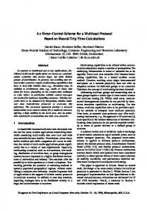
LAN 1 T C P S in k 1 HALM Sen der

SW 1

TCP 1

LAN 2 T C P S in k 2

0 .5 M b p s

SW 2 LAN 3

1 M bps

TC P 2

1 .5 M b p s TC P 3

SW 7

SW 3

LAN 4 SW 4

TC P 4

3 M bps

T C P S in k 4

4 M bps SW 5

TCP 5

LAN 5 SW 6

TCP 6

T C P S in k 5 LAN 6

A L A N w ith m H A L M re c e iv e rs

A. Simulations Results

T C P S in k 6

Fig. 4. Simulation topology.

20 48

10 24

Rate (Kbps)

We simulate HALM and LMSA protocols using the LBNL network simulator ns-2 [20]. The following default parameters are used in our simulations. All queues use FIFO drop-tail scheduling discipline with the maximum queuing delay of 0.15 sec. The link delay is set to 20 ms between two switches and 10 ms between a switch and an end system (a receiver or a sender). The TCP connections are modeled as FTP flows that always have data to send and last for the entire simulation time. A TCP-Reno flavor is used for simulating the congestion control behavior of TCP. The packet size is 500 bytes for both TCP and HALM. We choose a max-window of 4000 packets (2 MB) for TCP, which is sufficiently large to ensure TCP connections remain in the well-behaved mode. All simulations were run for 1000 seconds, which is long enough for observing transient and steady-state behaviors. The cumulative layer rates of a HALM source are initialized to {256,512,1024 Kbps}, and the lower bound of base layer rate is 220 Kbps. To keep our focus on the bandwidth allocation is for flows in the network, a linear utility function used in this set of simulations. On the receiver’s side, the initial , and 0 for . settings are 100 ms for 1) Performance in Heterogeneous Environments: Fig. 4 depicts the topology for our simulation. There is a HALM sender receivers belonging to six LANs, where each LAN and receivers. The bottleneck links are ( , ), has , and each one is shared between the HALM flow and to . To emulate a heterogea TCP connection from neous environment, the bottleneck bandwidths are set to 0.5, 1, 1.5, 2, 3, and 4 Mbps, respectively. Other links are sufficiently provisioned to ensure any drops are due to congestion at the bottleneck links. to 5. The receivers stay in In the first simulation, we set the session throughout the whole period. We observe that the receivers in the same LAN receive data at identical rates when local coordination is adopted. Therefore, from each LAN, we choose one receiver as a representative, and denote the receiver as receiver . Fig. 5 shows the cumulative layer from rates of the simulation, and Fig. 6 shows the bandwidth distribution between the competing HALM and TCP flows at different switches. We can see that basically the rates of layers 1, 2, and 3 adapt to the expected bandwidths of receivers 1, 3, and 5. If we

T C P S in k 3

2 M bps

51 2

25 6

Layer 3 Layer 2 Layer 1

12 8 0

100

200

300

400

500

600

700

800

900

1000

Time (s)

Fig. 5. Distribution of cumulative layer rates without joining and leaving.

assume that every HALM receiver expects a totally fair share of the bottleneck bandwidth with TCP traffic, this adaptation setting is just the one that maximizes the expected fairness index. However, due to some inaccuracy in bandwidth estimations, we can see oscillations of the layer rates. For instance, at time 225 s, 435 s, and 585 s, the rate of layer 3 adapts to receiver 6, because receiver 5 has given a relatively low bandwidth estimate while receiver 6 a higher one. As such, receiver 5 leaves layer 3 so that a higher expected degree of fairness is achieved. We also simulate LMSA-U and LMSA-E on this topology by replacing the corresponding HALM sender and receivers. The cumulative layer rates for LMSA-U and LMSA-E are set to and , respectively. The bandwidth distributions between TCP and layered traffic are compared in Table I. Compared to the receivers in the two static allocation-based schemes, a HALM receiver generally has a better share of bandwidth. Although some receivers, such as LMSA-U receiver 6, have a higher fairness index, the average fairness index of HALM is 0.84, which is noticeably higher than that of LMSA-U (0.67) and LMSA-E (0.69). Thus, as expected, HALM achieves higher performance in terms of the degree of the overall receiver satisfaction in a session.

95

500

1000

400

800

Bandwidth (Kbps)

Bandwidth (Kbps)


300

200

600

400

200

100

HALM TCP 0

0

200

400

600

800

HALM TCP 0

1000

0

200

400

Time (s)

800

1000

(c) Switch 3 2000

1200

1600

Bandwidth (Kbps)

Bandwidth (Kbps)

(a) Switch 1 1500

900

600

300

0

600

Time (s)

1200

800

400

HALM TCP

HALM TCP

0 0

200

400

600

800

1000

0

200

400

600

800

1000

Time (s)

Time (s) (c) Switch 3

(d) Switch 4 4000

3000

3500 2500 3000

Bandwidth (Kbps)

Bandwidth (Kbps)

2000

1500

1000

2500 2000 1500 1000

HALM TCP

500

HALM TCP

500 0

0 0

200

400

600

800

1000

0

200

400

600

Time (s)

Time (s)

(e) Switch 5

(f) Switch 6

800

1000

Fig. 6. Bandwidth distribution between HALM and TCP at different switches.

2) Performance With Dynamic Joining and Leaving: In this simulation, we let the receivers dynamically join and leave the session to observe the responsiveness of HALM. To fact out the effect of local coordination, we set to 1. In Table II, we show a joining/leaving schedule in our simulation. The corresponding source layer rates are shown in Fig. 7. We can see that HALM always tries to maximize the overall system performance (in terms of the expected fairness index) according

to the current bandwidth distribution of the session members. Since the joining and leaving actions are synchronized, the convergence time of HALM is very short. Usually, the time for a receiver to get the optimal share is within one control period, or about 15 s in this simulation. For example, after receiver 1 joins the session at 200 s, it waits for the control signal for 10 s, and then reports the expected bandwidth to the sender. After that, the rate of the base layer is adjusted to about 200 Kbps, which is the

96


TABLE I DISTRIBUTION OF THE RECEIVED BANDWIDTHS (Kbps). THE RATIO IS OBTAINED BY DIVIDING THE LAYERED STREAM BANDWIDTH BY THE TCP BANDWIDTH

HALM

Receiver

LMSA-U

BHALM

BTCP

Ratio

BLMSA-U

BTCP

Ratio

BLMSA-E

BTCP

Ratio

1

227.6

258.1

0.88

193.4

277.5

0.69

246.3

226.7

1.09

2

331.8

602.5

0.55

219.3

721.5

0.30

337.4

607.2

0.56

3

704.3

696.2

1.01

388.7

1025.2

0.38

487.7

895.5

0.54

4

705.9

1136.2

0.62

573.7

1303.9

0.43

701.2

1164.6

0.60

5

1472.4

1389.5

1.05

1317.8

1475.8

0.89

1003.6

1789.4

0.56

6

1582.1

2169.3

0.72

1725.8

1992.9

0.87

1004.3

2757.8

0.36

B. Statistical Results for Large Sessions

TABLE II SCHEDULE OF JOINING AND LEAVING

Receiver

1

2

3

4

5

6

Joining Time (s)

200

0

0

0

300

400

Leaving Time (s)

-

600

-

800

900

-

2048

Rate (Kbps)

1024

512

256 Layer 3 Layer 2 Layer 1

128 0

200

LMSA-E

400

600

800

1000

Time (s) Fig. 7. Distribution of cumulative layer rates with dynamic joining and leaving.

requirement of receiver 1, and the rates of layer 2 and 3 are also adjusted to maximize the overall system performance. We find that, after receiver 4 leaves the session at 800 s, the layer rates do not change significantly, as the original allocation still maximizes the expected fairness index with the new distribution. To the contrary, the departure of receiver 5 at 900 s triggers a totally new allocation: originally layer 3 is adapted to the expectation of receiver 5, but now it can adapt to that of receiver 6 to achieve a higher expected fairness index.

For large sessions, we directly model the bandwidths of the receivers in a session, , coming from different distributions. To emulate the heterogeneous nature, a commonly used tool is the mixture Gaussian model [27]. This model consists of clusters, where each cluster follows a Gaussian distribution. As we mentioned in Section I, The bandwidths are clustered because users use standard access technologies or share some bottlenecks. In our study, the cluster means are chosen from 100 Kbps to 3 Mbps. This range covers the bandwidths of many available network access and video compression standards. It is also a typical dynamic range of existing layered coders, such as the MPEG-4 PFGS coder [25]. The standard deviation of a cluster is set to 10% of the cluster mean. Therefore, most bandwidth fluctuations are within 10%, yet some are more than 50%, which reflects the dynamic nature of Internet traffic. In the following part, we present the results of three representative distributions, as listed in Table III. 1) Effect of Layering: In this experiment, we study the impact of layering on user fairness. We adopt a linear utility , and assume there are 512 uniformly spaced function operational points. The lower bound of the base layer rate is 128 Kbps, which is also the base layer rate for LMSA-U ; for and LMSA-E. For LMSA-U, is set to . LMSA-E allocation, is set to The relations between the expected fairness index and the number of layers are shown in Fig. 8. We observe that, compared to single-rate (only one layer) multicast, all these layered multicast schemes significantly improve the expected fairness index. One important question is how many layers should be used for a layered transmission system. From our results, it can be seen that the performance improvement, when using more than five layers, is marginal. Since using a large number of layers yields high computational complexity on both the sender and receiver’s sides, it is clear that three to five layers is a reasonable choice under a variety of session conditions. The optimal allocation algorithm in HALM exhibits much better performance and often outperforms the two static schemes by 10%–20% in terms of the expected fairness index.


97

k

TABLE III RECEIVER BANDWIDTH DISTRIBUTIONS FOR THE PERFORMANCE EVALUATION. : NUMBER OF CLUSTERS, : MEAN OF CLUSTER , : TOTAL NUMBER OF RECEIVERS, : NUMBER OF RECEIVERS IN CLUSTER

M

N

Distribution k

Mi (Kbps)

N

Ni

1

Clustered-1

3

200, 1000,2200

1000

333,333,334

2

Clustered-2

6

150, 500,900,1400,2000,2800

1000

166,166,167,167,167,167

3

Top-heavy

5

150,550,1100,1750,2650

1000

150,150,150,400,150

1.0

1.0

0.9

0.9

0.8

0.8

0.7 0.6 0.5 0.4 0.3

Optimal Allocation Exponential Allocation Uniform Allocation

0.2

0.7 0.6 0.5 0.4 0.3


0.2

0.1 0.0

i

Parameter Settings

Average Fairness Index


Order

iN

0.1 1

2

3

4

5

6

7

8

9

0.0

10

1

2

3

4

Number of Layers

5

6

7

8

9

10

Number of Layers

(a)

(b) 1.0 0.9


0.8 0.7 0.6 0.5 0.4 0.3 Optimal Allocation Exponential Allocation Uniform Allocation

0.2 0.1 0.0 1

2

3

4

5

6

7

8

9

10

Number of Layers

(c) Fig. 8. Average fairness indices of different allocation schemes with a linear utility function. (a) Clustered-1 distribution; (b) clustered-2 distribution; (c) top-heavy distribution.

This is because the optimal allocation algorithm allocates the layer rates according to the receiver bandwidth distributions. When the bandwidths are clustered, the layer rates can be adjusted to fit these clusters. On the contrary, static schemes may set the layer rates naively, e.g., set to a point with few receivers. This behavior can be observed from Table IV.

An interesting phenomenon due to the nonadaptability of the static schemes is that, the expected fairness index does not monotonically increase with . For example, in Fig. 8(c) with is the exponential allocation scheme, the performance of , and even of , 8. As proved in higher than that of Section IV-B, with the optimal allocation algorithm, increasing

98


TABLE IV ALLOCATED CUMULATIVE LAYER RATES FOR THE SECOND DISTRIBUTION (CLUSTERED-2, k = 6, M = f150; 500; 900; 1400; 2000; 2800g)

ρ L (Kbps) L

LMSA-U

LMSA-E

HALM

2

128, 1664

128, 625

128, 824

3

128, 1110, 2091

128, 368, 1065

128, 466, 1296

4

128, 864, 1600, 2336

128, 282, 625, 1378

128, 455, 853, 1855

5

128, 716, 1305, 1892, 2480

128, 240, 454, 853, 1610

128, 455, 824, 1296,1930

6

128, 618, 1108, 1598, 2088, 2578

128, 218, 368, 622, 1050, 1780,

128, 455, 824, 1285, 1855, 2564

the number of layers always leads to a higher degree of fairness. This also gives a justification for the use of sender-adaptation as a complement to the static allocation based adaptation schemes. To gain a better understanding of the behavior of these schemes, we also examine the distribution of individual fairness indices in a session. Fig. 9 shows the histograms of the fairness indices for the four bandwidth distributions with . It is clear that, with the optimal allocation scheme, the variances of individual fairness indices are reduced as well, because the optimal algorithm always tries to make the individual fairness indices close to 1, the maximum value. 2) Effect of Nonlinearity of Utility Functions: An important consideration in designing the application-aware fairness index is the nonlinear relation between the transmission bandwidth and perceptual video quality. To study the impact of this nonlinear nature, we model the utility function from the well established rate-distortion framework. Assume that the source statistics are Gaussian distributed, there is a closed-form solu, where tion for the rate-distortion function, when , and when [23]. This relationship offers a good approximation for practical encoders, and holds at the sequence, group of pictures and even frame level. We thus defined the utility function as the form , . In Fig. 10, and . we present the results with These parameters are calculated from the rate-distortion curve of the standard test sequence “Foreman” with the PFGS coder [25], where the video distortion is measured by Mean Square Error (MSE) and encoding rate is measured by Kbps. Compared with Fig. 8, the values of the optimal expected fairness indices with the nonlinear and the linear utility functions are quite close. However, as shown in Table V, the allocated layer rates under the optimal allocation are different. We have also conducted experiments with the utility functions of other video sequences. We find that, in general, the allocation granularity at lower rates is finer than that at higher rates with these nonlinear functions. This is because end-users do not perceive significant improvement in quality after a certain bit-rate. In other words, the perceptual quality saturates at high rates and, consequently, increasing the number of layers in this range may

result in a waste of bandwidth. This also explains why the exponential allocation often exhibits better performance than the uniform allocation with the nonlinear utility function, whereas its performance worsens with the linear utility function. C. Comparison of HALM and SAMM In this set of experiments, we compare HALM with a representative sender-adaptive layered multicast protocol, the SAMM protocol [5]. SAMM targets the future Internet with a priority-dropping scheme deployed at routers. Moreover, it attempts to build an overlaying network for scalable feedback collection by placing feedback mergers along a multicast tree. A feedback merger combines the bandwidth reports from its downstream receivers or mergers. In a merger, assume the number of distinct bandwidths reported from the downstream , a heuristic algorithm is then used to nodes is and iteratively remove entries. In each iteration, an entry removal that results in the highest Goodput is performed, where the Goodput is defined as the aggregate bandwidth delivered to the receivers. The trade-off between the FIFO drop-tail and priority dropping policies has been extensively studied in the literature [1], [2]. The proper choice is still subject to debate, and is really beyond the scope of this paper. Therefore, in the experiments, we focus on the comparisons of the rate allocation schemes of the two protocols, i.e., sampling-based in HALM and mergingbased in SAMM, and in particular, their accuracy in large-scale networks. Given the Internet topology modeling remains an open issue, we use three typical models to generate large-scale network topologies: Waxman [17], Inet [18], and Transit-Stub (TS) [19] models. The TS and Inet models reflect the hierarchical structure of the Internet from different aspects. The Waxman model, though not reflecting the structure of the real Internet, is attractive for its simplicity and is widely used to study networking problems. We perform simulations on three 6000-node networks generated by the above three models, respectively. Each network node represents a router; the sender is attached to a randomly selected node, and a receiver is attached to each of the remaining nodes.


99

450

450

400

400 Optimal Allocation Exponential Allocation Uniform Allocation

350


350

300

300

250

250

200

200

150

150

100

100

50

50

0

0 0

0.2

0.4

0.6

0.8

0

0.2

0.4

0.6

0.8

Fairness Index (b)

Fairness Index (a) 450 400 Optimal Allocation Exponential Allocation Uniform Allocation

350 300 250 200 150 100 50 0 0

0.2

0.4

0.6

0.8

Fairness Index (c) Fig. 9. Distributions of fairness indices of different allocation schemes with a linear utility function: X-axis: fairness index; Y-axis: number of receivers. Note that the figures are stacked histograms. (a) Clustered-1 distribution, L = 4; (b) clustered-2 distribution, L = 4; (c) top-heavy distribution, L = 4.

For HALM, the control bandwidth for sampling is set to 20 Kbps. For SAMM, we assume that a feedback merger is attached to each router. Note that the original SAMM (denoted as SAMM-GP) tries to maximize Goodput. This is different from the objective of HALM. To arrive at a fair comparison, we also simulated a variation of SAMM (denoted as SAMM-FI), which uses the same heuristic algorithm but the optimization objective in each iteration is to maximize the average fairness index. We also calculate the optimal allocation based on the exact and instant bandwidth distribution of all the receivers. Assume , and the expected fairness index under this allocation is the one under a practical algorithm (in HALM, SAMM-GP, or SAMM-FI) is , the accuracy of the practical algorithm is defined as . We first compare the accuracy of the three algorithms in a static scenario, where the delay of sampling or merging is assumed to be zero. We also assume that the background traffic is stationary, and a receiver’s expected bandwidth is uniformly distributed between 0.1 to 0.8 , where is the bottleneck bandwidth from the sender to the receiver. Therefore, errors in rate allocation are caused only by the limit of the sample size or the

merging algorithm. Fig. 11 shows the accuracy of the expected fairness index achieved in HALM, SAMM-GP, and SAMM-FI. We find that HALM and SAMM-FI both achieve high accuracy, and HALM is slightly better than SAMM-FI in all the topologies. The accuracy of SAMM-GP, however, is about 10% lower than theirs. This is simply because its objective is to maximize Goodput, not fairness. Hence, to obtain fair comparisons, in the following experiments, we consider SAMM-FI only. Intuitively, by using hierarchically organized mergers, SAMM should exhibit better responsiveness. This is validated in Fig. 12, which shows the average time for collecting the samples in HALM, as well as that for merging all the receiver reports along a multicast tree in SAMM. For SAMM, the collections for all three topologies are done in reasonably short times, although the times for Inet and TS are slightly shorter as they are resticted hierarchical topologies. Not surprisingly, it takes much longer time (nearly 5 s) for a HALM sender to collect the feedbacks. In a highly dynamic environment, a long collection time would result in skewness between a receiver’s current expected bandwidth and its recent report. To investigate the impact of such skewness, we perform an experiment using settings


1.0

1.0

0.9

0.9

0.8

0.8

0.7

0.7



100

0.6 0.5 0.4 0.3


0.2

0.5 0.4 0.3


0.2

0.1 0.0

0.6

0.1 1

2

3

4

5

6

7

8

9

0.0

10

1

2

3

4

Number of Layers

5

6

7

8

9

10

Number of Layers

(b)

(a) 1.0 0.9


0.8 0.7 0.6 0.5 0.4 0.3


0.2 0.1 0.0

1

2

3

4

5

6

7

8

9

10

Number of Layers

(c) Fig. 10. Average fairness indices of different allocation schemes with a nonlinear utility function. (a) Clustered-1 distribution; (b) Clustered-2 distribution; (c) Top-heavy distribution.

ρ L* (Kbps)

L

Linear Utility Function

Non-linear Utility Function

2

128, 841

128, 824

3

128, 466, 1325

128, 466, 1296

4

128, 288, 628, 1389

128, 455, 853, 1855

5

128, 455, 841, 1325, 1896

128, 455, 824, 1296,1930

6

128, 455, 841, 1325, 1855, 2616

128, 455, 824, 1285, 1855, 2764

similar to that for the original SAMM performance evaluation (See [5], Section V-B for details). Specifically, the background traffic is generated using a 2000-state Markov Modulated Poisson Processes (MMPPs). The state transition rates are varied from 0 to 120 s , and the higher the transition rate the more dynamic the traffic. From Fig. 13, it can be seen that

100 Accuracy (%)

TABLE V OPTIMAL ALLOCATIONS WITH THE LINEAR AND NON-LINEAR UTILITY FUNCTIONS FOR THE SECOND DISTRIBUTION (CLUSTERED-2, k = 6, M = f150; 500; 900; 1400; 2000; 2800g)

80 HALM SAMM-FI SAMM-GP

60 40 20 0 Waxman

Fig. 11.

Inet Topology

TS

Accuracy of HALM, SAMM-FI, and SAMM-GP in a static scenario.

HALM exhibits better performance in static scenarios, but gets worse in highly dynamic scenarios because of the skewness. On the contrary, SAMM is reasonably stable, due to its fast responsiveness in feedback collection. Nevertheless, the main rationale for adopting sampling in HALM is to be compatible to the best-effort Internet; thus no involvement of intermediate nodes is advocated.


Report Collection Time(ms)s

5000

4000

3000 HALM

101

time and accuracy of sampling and how to accommodate deviations in TCP throughput estimation (e.g., existing models does not work well with high loss rate, and tends to penalize receivers with longer RTTs even if they are behind the same bottleneck with others).

SAMM-FI 2000

ACKNOWLEDGMENT 1000

The authors would like to thank the researchers at the Wireless and Networking Group, Microsoft Research, Asia (MSRA), for discussions about layered video transmission, and the researcher at the Internet Media Group, MSRA, for discussions about the PFGS coding. Furthermore, the comments from the anonymous reviewers were a great help for improving this paper.

0 Waxman

Fig. 12.

Inet Topology

TS

Report collection times of HALM and SAMM-FI.

100

REFERENCES

Accuracy(%)

80 60 40

HALM SAMM-FI

20 0 0

30

60

90

1200

Transition Rate (1/s)

Fig. 13.

Accuracy of HALM and SAMM-FI in dynamic scenarios.

VII. CONCLUSIONS AND FUTURE WORK In this paper, we have presented a hybrid adaptation protocol for layered video multicast. The protocol, known as HALM, performs adaptations on both the sender and the receiver’s sides to improve intra-session fairness as well as TCP-friendliness. Our main contribution is a formal study on the sender-based optimal layer rate allocation and its practical use. We have defined optimization criteria and derived a scalable algorithm to solve the problem. We have also discussed the implementation issues for HALM; specifically, the choice of the layered video coder, the estimation of TCP-friendly bandwidth, and the inference of bandwidth distribution. The performance of HALM has been evaluated under a variety of configurations. We have also compared it with traditional static allocation based protocols. Our results show that HALM interacts with TCP substantially better than traditional protocols, outperforming them by 10–20% or more in terms of the expected fairness index. With the optimal allocation algorithm, increasing the number of layers always leads to better performance, and usually three to five layers offer a satisfactory degree of fairness. However, we found that this appealing property does not hold with a static allocation. Our future work is to conduct more simulations and real experiments with advanced layered coding algorithms (such as the MPEG-4 PFGS codec [25]). This also enables more extensive and realistic comparisons with other layered multicast protocols. Other potential work includes how to improve the response

[1] S. McCanne, V. Jacobson, and M. Vetterli, “Receiver-driven layered multicast,” in Proc. ACM SIGCOMM 96, Aug. 1996, pp. 117–130. [2] S. Bajaj, L. Breslau, and S. Shenker, “Uniform versus priority dropping for layered video,” in Proc. ACM SIGCOMM 98, Sept. 1998, pp. 131–143. [3] X. Li, M. Ammar, and S. Paul, “Video multicast over the internet,” IEEE Network Mag., vol. 13, no. 2, pp. 46–60, Apr. 1999. [4] J. Bolot, T. Turletti, and I. Wakeman, “Scalable feedback control for multicast video distribution in the internet,” Comput. Commun. Rev., vol. 24, no. 4, pp. 58–67, Oct. 1994. [5] B. Vickers, C. Albuquerque, and T. Suda, “Source adaptive multi-layered multicast algorithms for real-time video distribution,” IEEE/ACM Trans. Networking, vol. 8, no. 6, pp. 720–733, Dec. 2000. [6] B. Li and J. Liu, “Multi-rate video multicast over the internet: an overview,” IEEE Network, Special Issue on Multicasting: An Enabling Technology, vol. 17, no. 1, pp. 24–29, Jan. 2003. [7] L. Vicisano, L. Rizzo, and J. Crowcroft, “TCP-like congestion control for layered multicast data transfer,” in Proc. IEEE INFOCOM 98, Apr. 1998, pp. 996–1003. [8] D. Rubenstein, J. Kurose, and D. Towsley, “The impact of multicast layering on network fairness,” in Proc. ACM SIGCOMM 99, Sept. 1999, pp. 27–38. [9] S. Sarkar and L. Tassiulas, “Distributed algorithms for computation of fair rates in multirate multicast trees,” in Proc. IEEE INFOCOM 2000, Apr. 2000. [10] J. Padhye, V. Firoiu, D. Towsley, and J. Kurose, “Modeling TCP throughput: a simple model and its empirical validation,” in Proc. ACM SIGCOMM 98, Sept. 1998. [11] T. Turletti, S. Parisis, and J. Bolot, “Experiments With a Layered Transmission Scheme Over the Internet,” INRIA, Tech. Rep. N’3296, Nov. 1997. [12] D. Sisalem and A. Wolisz, “MLDA: a TCP-friendly congestion control framework for heterogeneous multicast environments,” in Proc. 8th Int. Workshop on Quality of Service (IWQoS), June 2000. [13] S. Floyd, M. Handley, J. Padhye, and J. Widmer, “Equation-based congestion control for unicast applications,” in Proc. ACM SIGCOMM 2000, Aug. 2000, pp. 43–57. [14] N. Shacham, “Multipoint communication by hierarchically encoded data,” in Proc. IEEE INFOCOM 92, May 1992, pp. 2107–2114. [15] D.-P. Wu, Y.-T. Hou, W. Zhu, Y.-Q. Zhang, and J. Peha, “Streaming video over the internet: approaches and directions,” IEEE Trans. Circuits Syst. Video Technol., vol. 11, no. 3, pp. 282–300, Mar. 2001. [16] S. Gorinsky, K. K. Ramakrishnan, and H. Vin, “Addressing Heterogeneity and Scalability in Layered Multicast Congestion Control,” Univ. Texas, Austin, Tech. Rep. TR2000-31, Nov. 2000. [17] B. M. Waxman, “Routing of multipoint connections,” IEEE J. Select. Areas Commun., vol. 6, no. 9, pp. 1617–1622, 1988. [18] P. Francis, S. Jamin, C. Jin, Y. Jin, D. Raz, Y. Shavitt, and L. Zhang, “IDMaps: a global internet host distance estimation service,” IEEE/ACM Trans. Networking, vol. 9, pp. 525–540, Oct. 2001. [19] E. W. Zegura, K. Calvert, and S. Bhattacharjee, “How to model an internetwork,” in Proc. IEEE INFOCOM 96, Apr. 1996.

102

[20] S. McCanne and S. Floyd. The LBNL Network Simulator, ns-2. [Online] Available http://www.isi.edu/nsnam/ns/ [21] G. Schuster and A. Katsaggelos, Rate-Distortion Based Video Compression. Norwell, MA: Kluwer, 1997. [22] W. Stevens, TCP/IP Illustrated. Reading, MA: Addison-Wesley, 1997, vol. 1, The Protocols. [23] H.-M. Hang and J.-J. Chen, “Source model for transform video coder and its application,” IEEE Trans. Circuits Syst. Video Technol., vol. 7, pp. 287–311, Apr. 1997. [24] W. Li, “Overview of the fine granularity scalability in MPEG-4 video standard,” IEEE Trans. Circuits Syst. Video Technol., vol. 11, pp. 301–317, Mar. 2001. [25] S. Li, F. Wu, and Y.-Q. Zhang, “Experimental results with Progressive Fine Granularity Scalable (PFGS) Coding,”, ISO/IEC JTC1/SC29/WG11, MPEG99/m5742, Mar. 2000. [26] D. Montgomery and G. Runger, Applied Statistics and Probability for Engineers. New York: Wiley, 1994. [27] D. Titterington, A. Smith, and U. Makov, Statistical Analysis of Finite Mixture Distributions. New York: Wiley, 1985. [28] H. Schulzrinne, S. Casner, R. Frederick, and V. Jacobson, “RTP: a transport protocol for real-time applications,” in RFC 1889, Jan. 1996. [29] M. Speer and S. McCanne, RTP usage with layered multimedia streams, in Internet Draft, Dec., 20 1996. [30] Y. Yang, M. Kim, and S. Lam, “Optimal partitioning of multicast receivers,” in Proc. IEEE ICNP’00, Nov. 2000.

Jiangchuan Liu (S’01–M’03) received the B.Eng degree (cum laude) from Tsinghua University, Beijing, China, in 1999, and the Ph.D. degree from The Hong Kong University of Science and Technology in 2003, both in computer science. He is currently an Assistant Professor in the Department of Computer Science and Engineering, The Chinese University of Hong Kong. In the summers of 2000–2002, he had internships with Microsoft Research, Asia, working on video multicast over the Internet and service discovery in variable topology networks. He is a recipient of Microsoft research fellowship and a co-inventor of one European patent (granted) and two U.S. patents (pending). His current research interests include multicast protocols, streaming media, wireless ad hoc networks, and service overlay networks. He won first-class honors in several regional and national programming contests. He was a TPC member and Information System Co-Chair for IEEE Infocom’04.


Bo Li (S’89–M’92–SM’99) received the B.S. (summa cum laude) and M.S. degrees in the computer science from Tsinghua University, Beijing, China, in 1987 and 1989, respectively, and the Ph.D. degree in the computer engineering from the University of Massachusetts, Amherst, in 1993. Between 1994 and 1996, he worked on high performance routers and ATM switches in IBM Networking System Division, Research Triangle Park, NC. Since then, he has been with the Computer Science Department, Hong Kong University of Science and Technology, where he is now an Associate Professor. He is also an Adjunct Researcher at Microsoft Research Asia (MSRA). His current research interests include wireless mobile networking supporting multimedia, video multicast and all optical networks using WDM. He co-authored the first paper on proxy server placement in 1999. He has been an editorial board member of the ACM Journal of Wireless Networks (WINET), ACM Mobile Computing and Communications Review (MC2R), SPIE/Kluwer Optical Networking Magazine (ONM). He served as a guest editor for ACM Performance Evaluation Review Special Issue on Mobile Computing (December 2000), and SPIE/Kluwer Optical Networks Magazine Special Issue on Wavelength Routed Networks: Architecture, Protocols and Experiments (January/February 2002). Dr. Li has been on editorial board for IEEE TRANSACTIONS ON WIRELESS COMMUNICATIONS, IEEE TRANSACTIONS ON VEHICULAR TECHNOLOGY, IEEE JOURNAL OF SELECTED AREAS IN COMMUNICATIONS (JSAC)—Wireless Communications Series, KICS/IEEE JOURNAL OF COMMUNICATIONS AND NETWORKS (JCN). He served as a guest editor for IEEE Communications Magazine Special Issue on Active, Programmable, and Mobile Code Networking (April 2000), IEEE JOURNAL ON SELECTED AREAS IN COMMUNICATIONS Special Issue on Protocols for Next Generation Optical WDM Networks (October 2000). Currently, he is the lead guest editor for a special issue of IEEE JOURNAL ON SELECTED AREAS IN COMMUNICATIONS on Recent Advances in Service-Overlay Network, and a guest editor for a special issue of IEEE JOURNAL ON SELECTED AREAS IN COMMUNICATIONS on Ad Hoc Networks. In addition, he has been involved in organizing over 30 conferences, especially IEEE Infocom, since 1996.

Ya-Qin Zhang (S’87–M’90–SM’93–F’98) received the B.S. and M.S. degrees in electrical engineering from the University of Science and Technology of China (USTC), Hefei, in 1983 and 1985, and the Ph.D degree in electrical engineering from George Washington University, Washington, DC, in 1989. He also had executive business training from Harvard University, Cambridge, MA. He joined Microsoft Research China in January 1999, leaving his post as the Director of Multimedia Technology Laboratory at Sarnoff Corporation, Princeton, NJ (formerly David Sarnoff Research Center, and RCA Laboratories). He has been engaged in research and commercialization of MPEG2/DTV, MPEG4/VLBR, and multimedia information technologies. He was with GTE Laboratories, Inc., Waltham, MA, and Contel Technology Center, Chantilly, VA, from 1989 to 1994. He has authored and coauthored over 200 refereed papers in leading international conferences and journals. He has been granted over 40 U.S. patents in digital video, Internet, multimedia, wireless, and satellite communications. Many of the technologies he and his team developed have become the basis for start-up ventures, commercial products, and international standards. He serves on the Board of Directors of five high-tech IT companies. Dr. Zhang served as the Editor-In-Chief for the IEEE TRANSACTIONS ON CIRCUITS AND SYSTEMS FOR VIDEO TECHNOLOGY from July 1997 to July 1999. He was the Chairman of Visual Signal Processing and Communications Technical Committee of IEEE Circuits and Systems. He serves on the editorial boards of seven other professional journals and over a dozen conference committees. He has been a key contributor to the ISO/MPEG and ITU standardization efforts in digital video and multimedia. He has received numerous awards, including several industry technical achievement awards and IEEE awards such as CAS Jubilee Golden Medal. He was awarded as the “Research Engineer of the Year” in 1998 by the Central Jersey Engineering Council for his “leadership and invention in communications technology, which has enabled dramatic advances in digital video compression and manipulation for broadcast and interactive television and networking applications.” He received the prestigious national award as “The Outstanding Young Electrical Engineer of 1998,” given annually to one electrical engineer in the United States.