Multispectral Remote Sensing Image Classification Using Wavelet ...

Chapter 1 Multispectral Remote Sensing Image Classification Using Wavelet Based Features Saroj K. Meher, Bhavan Uma Shankar and Ashish Ghosh Machine Intelligence Unit Indian Statistical Institute 203 B. T. Road Kolkata 700108, India {saroj t,uma,ash}@isical.ac.in

1 Introduction Multispectral remotely sensed images composed information over a large range of variation on frequencies (information) and these frequencies change over different regions (irregular or frequency variant behavior of the signal) which need to be estimated properly for an improved classification [1, 2, 3]. Multispectral remote sensing (RS) image data are basically complex in nature, which have both spectral features with correlated bands and spatial features correlated within the same band (also known as spatial correlation). An efficient method for utilization of these spectral and spatial (contextual) information can improve the classification performance significantly compared to the conventional non-contextual information based methods. In general, the spectral component of a remotely sensed image pixel may be a mixture of more than one spectral information that usually comes from the different regions of the study area. However, the conventional multispectral remotely sensed image classification systems detect object classes only according to the spectral information of the individual pixel/pattern in a particular frequency band, while a large amount of spatial and spectral information of neighboring pixels of different regions at other frequency bands are neglected. Hence the pixels are classified based on its spectral intensities of a specific band and does not give attention to its spatial and spectral dependencies and thus the spectral intensities of the neighbors at different frequency bands are assumed to be independent. Such approaches may be reasonable if spatial resolution is high or when the spectral intensities are well separated for different classes, which is rarely found in any real life data sets. For example, in the classification of urban areas, the densities of the spectral intensities are seldom well separated. Thus it is important to decide whether the arrangements of spatial data can be used as features directly in its original form or with a set of extracted features obtained through any feature-extraction method where, the information S.K. Meher et al.: Multispectral Remote Sensing Image Classification Using Wavelet Based Features, StudFuzz 210, 3–34 (2007) c Springer-Verlag Berlin Heidelberg 2007 www.springerlink.com

4

S.K Meher et al.

are uncorrelated both in spatial and spectral domain to separate the data into desired classes. Many research efforts have been made to take the advantages of neighboring pixel information (texture feature information [1, 4, 5]) and applied for the classification of remotely sensed data. These include texture features extracted from angular second moments, contrast, correlation, entropy, variance, etc., computed from the gray level co-occurrence matrices [4]. These extracted texture features play an important role and help to increase the performance of the classifier. However, these methods are computationally expensive due to the estimation of autocorrelation parameters and transition probabilities. Also, the texture elements are not easy to quantify and it deals with the spatial distribution of the gray levels over a portion of an image. Later Gaussian Markov random fields (GMRF) [6, 7, 8] and Gibbs random fields [9] were proposed to characterize textures. Further, local linear transformations are also used to compute texture features [10]. These conventional statistical approaches to texture analysis such as co-occurrence matrices, second order statistics, GMRF and local linear transforms are restricted to the analysis of spatial interactions over relatively small neighborhoods on a single scale. As a matter of fact, their performance is best for the analysis of micro-textures only [11]. Apart from the texture feature extraction, various other aspects like uncorrelation of spectral information called as spectral unmixing, subpixel analysis and super resolution [12, 13, 14], spectral angle mapping are the important methods of exploring the spectral and spatial behavior of pixels. A brief review of spectral unmixing methods have been described by Keshava and Mustard in [15]. Brown et al. [16] proposed a support vector Machines based spectral unmixing and made a comparison with the linear spectral mixture models (LSMMs) and artificial neural networks. Chang and Ren in [17] performed a comparative study of mixed pixel classification algorithms. In an another study, Faraklioti and Petrou [18] described an statistical approach of spectral unmixing named as illumination invariant unmixing of sets of mixed pixels for classification. Shah and Varshney [19] proposed an higher order statistical approach to spectral unmixing of remote sening imagery, that is derived from independent component analysis [20, 21, 22]. In [23], Burke et al. described the application of parametric feature extraction and classification strategy for braincomputer interfacing. Song in [24] described the spectral mixture analysis for subpixel vegetation fractions in the remote sensing environmental analysis. An automated extraction of endmember (uncorrelated synthesized information) in both spatial and spectral domain for multidimensional morphological operations has been described by Plaza et al. [25], where the authors proposed a new automated method that performs unsupervised pixel purity determination and endmember extraction from multidimensional datasets, which is achieved with the use of both spatial and spectral information. In a similar context, Subpixel analysis is another important method of information extraction from a pixel. In this regard Barducci et al. [26] described the performance and the characteristics of a new algorithm for subpixel image

Wavelets for Multispectral Image Classification

5

classification, performed by means of a fully constrained least-squares estimator operated with a multi-resolution approach in the framework of the linear mixing model. Broadwater et al. [27] described a hybrid algorithm for subpixel detection in hyperspectral imagery, where the hybrid detector based on both adaptive matched subspace detector and fully constrained least squares was developed to take the advantage of each detectors strengths. In a soft computing paradigm, Tatem et al. [28] described a super-resolution land cover pattern prediction using a Hopfield neural network. Weiguo et al. [29] proposed an adaptive resonance theory MAP (ARTMAP) neural network based mixture analysis model for subpixel classification of land covers in remote sening images. Pastina et al. [30] described a two-dimensional super-resolution spectral analysis applied to synthetic aperture radar images, where he discussed a technique for improving the geometrical resolution of the image with respect to the numerical values related to the compressed coded waveform and the synthetic aperture, so that subsequent classification procedures will have improved performance as well. A super resolution feature extraction techniques for military and civilian applications such as the detection and classification of moving targets in strong clutter background have been described in [31]. Foody et al. [32], described a super-resolution mapping of the shoreline through soft classification analysis, where they applied simulated annealing to the output of a soft classification. In a similar approach of information extraction, spectral angle mapping model has been used for rapid assessment of soil salinization in arid area [33]. However, in the conventional multispectral image classification method, the pixel information in either of spectral or spatial/textural domain are usually not sufficient to discriminate properly the different land cover classes. Hence, use of both spectral and textual information in classification problem is more appropriate. In this regard, many approaches like spectral unmixing, subpixel classification, etc. as discussed above have been adopted in the literature. Some attempts were also been made to use both spectral and textual features [5, 34, 35, 36, 37]. But, the texture feature extraction based on these methods normally assume the stationarity of the texture within the analysis range and hence may not be much useful. For this reason the characterization of the texture should be in both spatial and frequency domains simultaneously. One efficient way to deal with such problems is to recognize the image by a number of subsampled approximations of it at different resolutions and desired scales. This approach is conventionally called multiresolution and/or filter bank analysis [38, 39]. In this analysis particularly, Gabor filters and wavelet transform (WT) have received a lot of attention [11, 40, 41, 42]. However, a major disadvantage in using Gabor transform is that the output of Gabor filter banks are not mutually orthogonal, which may result in a significant correlation between texture features. Moreover, these transformations are usually not reversible, which limits their applicability for texture synthesis. Using the WT, which provides a precise and unifying framework for the analysis and characterization of a signal at different scales [11], most of these

6

S.K Meher et al.

disadvantages can be avoided. Another advantage of WT over Gabor filter is that, the low pass and high pass filters used in the WT remain the same between two consecutive scales while the Gabor approach requires filters of different parameters [40]. In other words, Gabor filters require proper tuning of filter parameters at different scales. As discussed above, to capture the local variations in the orientation and frequency of texture elements that lead to the large scale frequency variation behavior of remotely sensed image textures, we need a joint spatial and frequency representation. In this regard, WT is found to be a promising tool for texture analysis in both spatial and frequency domains [43] simultaneously, as it has the ability to examine the signal at different scales. This means, the WT represents the input information in both spatial and frequency domain in a combined manner. The WT scheme thus, analyzes the coarse image first and gradually increases the resolution to analyze the finer details. Basically the WT coefficients represent the characteristic in sub-frequency bands, indicating the characteristic of the original pixel information in that location from where the WT coefficients originated. Thus the WT coefficients obtain neighboring pixels information that are uncorrelated in spatial domain. Hence the use of classification methods with these coefficients instead of original pixel value or the pixel with extracted features either in the spatial or spectral domain separately is more justifiable. These characteristics of the WT motivates us to use it for extraction of hidden features from images taken from remote sening imagery with large scale frequency variation behavior of the pixels. Research works related to texture classification using WT [11, 41] has already been carried out. Also the use of statistical correlation based features in the WT domain for classification have also been reported in [42, 44]. In a similar approach, some research studies have been made to use WT for target classification of remote sensing images [45, 46]. A comparative study of multiwavelet [47, 48], wavelet, and shape features [4], for microcalcification classification in mammogram has been described in [49], where it is experimentally shown that the results of multiwavelet based approach were better compared to wavelet and statistical based feature. However the computational complexities of multiwavelet based classification is much higher than the wavelet based one. In the present work we have tried to explore the advantages of WT, instead of multiwavelet and statistical based approaches, by incorporating it as a preprocessor in both non-fuzzy [50] and fuzzy classifiers [51, 52, 56, 57]. In this method we first extract features of the input patterns/pixels using WT and use these features for the next stage of classification. We have evaluated the performance of the WF based classification methods with different wavelets. Six classifiers are used for the performance evaluations of the wavelet and original feature based methods. Two of them are from non-fuzzy and the rest four from fuzzy. In the non-fuzzy cases, the simple and most popular classifiers known as: conventional maximum likelihood (ML) [50] and k-nearest neighbor (k-NN) [53] are used. Similarly in the fuzzy domain, we have considered the fuzzy version of the non-fuzzy classifiers considered above i.e.,


7

fuzzy ML (FML) [54] and fuzzy k-NN (Fk-NN) [55]. The intention behind the consideration of the fuzzy version of non-fuzzy classifiers is that, a comparative performance can also be made in both WF based fuzzy and non-fuzzy classifiers. In addition to these, we have also used two newly developed fuzzy classifiers known as, fuzzy product aggregation reasoning rule (FPARR) proposed by Ghosh et al. [56] and and fuzzy explicit (FE) method proposed by Melgani et al. [57]. Comparison of classification results showed that the WF based classification scheme is yielding superior performance with all wavelets and classifiers. However the performance of the classifiers are better with biorthogonal wavelets. All the classifiers are tested on three multispectral remote sening images; two four-band Indian Remote Sensing 1A (IRS-1A) satellite images and one three-band SPOT image [58] for land covers classification. The organization of the chapter is as follows. Section 2, describes the wavelet transform based feature extraction method. Different non-fuzzy and fuzzy classifiers have been discussed in Section 3. A brief discussion of performance analysis index has been made in Section 4. Section 5 summarized the comparative results with discussion. Finally a concluding remark is made in Section 6.

2 Wavelet transformation based feature extraction To deal with the frequency variation behavior of signals in an appropriate way, many research efforts have been made. Efforts are made to overcome the disadvantages of the Fourier transform (FT) [39, 43], which assumes the signal to be stationary (frequency invariant) within its total range of analysis. WT [38, 39, 43, 59] is an example of such a transform. The most important difference of the WT from FT is that the time localization of the signal frequencies will not be lost. This problem can be sorted out to some extend using short time FT (STFT) [39]. However, the selection of window is a main problem in STFT. As, narrow windows give good time resolution, but poor frequency resolution and wide windows give good frequency resolution, but poor time resolution; furthermore, wide windows may violate the condition of stationarity. The problem, in fact, is the selection of window function once and use that window in the entire analysis. The WT on the other hand is an extension of these transforms. Prominent frequencies in the original signal will appear as high amplitude in the region of the wavelet transformed signal that includes those frequencies. If the main information of the signal lies in the high frequency region, as happens most often, the time localization of these frequencies will be more precise, since they are characterized by more number of samples. If the main information lies only at very low frequency regions, the time localization will not be very precise, since few samples are used to express signal at these frequencies. This procedure in effect offers a good time resolution at high frequencies, and good frequency resolution at low frequencies.

8

S.K Meher et al.

WT basically extends single scale analysis to multiscale analysis. The multiscale behavior of the WT analyze or decompose the signal in multiple number of scales, where each scale represents a particular coarseness of the analyzed signal. Thus the decomposition steps divide the signal into a set of signals of varying coarseness ranging from low frequency to high frequency components. Accordingly the WT tries to identify both the scale and space information of the events simultaneously. This makes the WT useful for signal feature analysis. This property is more useful for remote sensing data analysis, where, any characteristic of the scene is first analyzed using low resolution and then analyze an area of interest in detail using an appropriate higher resolution level. Since we are dealing with irregular textures of remotely sensed images, the decomposition of the signal into different scales, which can uncorrelate the data as much as possible without losing their main distinguishable characteristic is particularly more useful when the WT is done on an orthogonal basis [38]. The orthogonal basis is more compact in its representation, as it allows the decomposition of the underlaying space into orthogonal subspaces, which makes it possible to ignore some of the decomposed signals. WT is also suitable for operations like feature extraction [60, 61], parameter estimation [62, 63] and exact reconstruction of the signal series because of its invertible properties [38, 39]. WT is identical to a hierarchical subband system, where the subbands are logarithmically spaced in frequency. The wavelets are the functions used in the transformation which act as a basis for representing many functions of the same family. A series of functions can be generated by translation and dilation of these functions called mother wavelets ψ(x). The translation and dilation of the mother wavelet can be given by t−τ −1/2 ψ , γ = 0 and, γ ε R, τ ε R (1) ψγ,τ (t) = |γ| γ where τ and γ are the translation and dilation parameters, respectively. R is any real number. We have tested the classification of the remote sensing images using wavelets from different (Daubechies, Biorthogonal, Coiflets, Symlets) groups [59], however results are given for four wavelets as their performances are comparatively (empirically) better than others. These are Daubechies 3 (Db3), Daubechies 6 (Db6), Biorthogonal 3.3 (Bior3.3) and Biorthogonal 3.5 (Bior3.5) wavelets [59]. In Daubechies wavelets, N (3 or 6) is related to support width, filters length, regularity and number of vanishing moments for the wavelets. For example, DbN is having support width of 2N − 1, filter length (number of filter coefficients) of 2N , regularity about 0.2N for large N and number of vanishing moments is N. Similarly, 3.3 and 3.5 of biorthogonal wavelets indicate some properties like regularities, vanishing moments, filter length etc. The filter coefficients for the decomposition (g as lowpass ˜ as highpass) of and h as highpass) and reconstruction (˜ g as lowpass and h


9

these four wavelets [59] are given in Tables 1 and 2. These wavelets are implemented with the multiresolution scheme given by Mallat [38], which is briefly described below. Table 1. Decomposition and reconstruction filter coefficients for Db3 and Db6 wavelet bases [59] No. of filter coefficients 0 1 2 3 4 5 6 7 8 9 10 11 12

Db3 Decomposition Reconstruction ˜ g h g˜ h 0.0352 -0.3327 0.3327 0.0352 -0.0854 0.8069 0.8069 0.0854 -0.1350 -0.4599 0.4599 -0.1350 0.4599 -0.1350 -0.1350 -0.4599 0.8069 0.0854 -0.0854 0.8069 0.3327 0.0352 0.0352 -0.3327 -

Db6 Decomposition Reconstruction ˜ g h g˜ h -0.0011 -0.1115 0.1115 -0.0011 0.0048 0.4946 0.4946 -0.0048 0.0006 -0.7511 0.7511 0.0006 -0.0316 0.3153 0.3153 0.0316 0.0275 0.2263 -0.2263 0.0275 0.0975 -0.1298 -0.1298 -0.0975 -0.1298 -0.0975 0.0975 -0.1298 -0.2263 0.0275 0.0275 0.2263 0.3153 0.0316 -0.0316 0.3153 0.7511 0.0006 0.0006 -0.7511 0.4946 -0.0048 0.0048 0.4946 0.1115 -0.0011 -0.0011 -0.1115

Table 2. Decomposition and reconstruction filter coefficients for Bior3.3 and Bior3.5 wavelet bases [59] No. of filter Coefficients 0 1 2 3 4 5 6 7 8 9 10 11 12

Bior3.3 Decomposition Reconstruction ˜ g h g˜ h 0.0663 0 0 0.0663 -0.1989 0 0 0.1989 -0.1547 -0.1768 0.1768 -0.1547 0.9944 0.5303 0.5303 -0.9944 0.9944 -0.5303 0.5303 0.9944 -0.1547 0.1768 0.1768 0.1547 -0.1989 0 0 -0.1989 0.0663 0 0 -0.0663 -

Bior3.5 Decomposition Reconstruction ˜ g h g˜ h -0.0138 0 0 -0.0138 0.0414 0 0 -0.0414 0.0525 0 0 0.0525 -0.2679 0 0 0.2679 -0.0718 -0.1768 0.1768 -0.0718 0.9667 0.5303 0.5303 -0.9667 0.9667 -0.5303 0.5303 0.9667 -0.0718 0.1768 0.1768 0.0718 -0.2679 0 0 -0.2679 0.0525 0 0 -0.0525 0.0414 0 0 0.0414 -0.0138 0 0 0.0138

10

S.K Meher et al.

2.1 Discrete WT and multiresolution analysis 1-Dimensional The discrete WT analyzes the signal at different frequency bands with different resolutions by decomposing the signal into low frequency (approximation) and high frequency (details) band information. WT employs two sets of functions, called scaling functions and wavelet functions, which are associated with low pass and highpass filters, respectively. The decomposition of the signal into different frequency bands is obtained by successive highpass and lowpass filtering of the signal. The 1-dimensional (1-D) original signal, (e.g., sn = [snk ]) is decomposed using a highpass filter hk and a lowpass filter gk , where n = 1, 2, ...Q is the number of decomposition levels and k = 1, 2, ...S is the number of signal samples. The decomposed signals consist of two parts sn−1 and dn−1 , called the smooth or lowpass and fine or highpass information. The two decomposed signal can be expressed as sn−1,j =

S

snk .gk−2j ,

(2)

snk .hk−2j

(3)

k=1

dn−1,j =

S k=1

with j as the length of the convolution masks. The reconstruction of the original signal from the decomposed WT coefficients can be performed as ˜ k−2j ]. [sn−1,j .˜ gk−2j + dn−1,j .h (4) snk = j

where g˜k and h˜k are the reconstruction filter coefficients. The convolution operation between two discrete sequences, e.g., y and z, as in Eqs. (2) and (3), can be expressed as CNV = y ∗ z. Here y and z represents the signal and wavelet filter sequences and their convolution operation can be defined as CN V j =

S

yk .zj−k .

(5)

k=1

The notation (↓ 2)y in Fig. 1 denotes the downsampled version of the sequence y by 2, i.e., ((↓ 2)y)k = y2k . Here the odd-numbered WT coefficients are dropped and the even-numbered WT coefficients are renumbered. The notation (↑ 2)y in Fig. 2 denotes the upsampled version of the sequence y by 2, i.e., ((↑ 2)y)2k = yk , ((↑ 2)y)2k+1 = 0.


11

Here a zero is inserted between each pair of adjacent WT coefficients and re-numbered. Thus the decomposition step consisted of two discrete convolution operations as (h ∗ sn )j =

S

snk .h( j − k), and

(6)

k=1

(g ∗ sn )j =

S

snk .g( j − k).

(7)

k=1

where ∗ represents the convolution operation. This convolution operation is followed by downsampling as sn−1 = (↓ 2)(g ∗ sn ), dn−1 = (↓ 2)(h ∗ sn ).

(8) (9)

The reconstruction step consists of upsampling, followed by two convolution operations. The reconstruction of the original signal can be expressed as sn = Reconstructed low f requency part of the signal(RLF P S) + Reconstructed high f requency part of the signal(RHF P S) ˜ ∗ (↑ 2)dn−1 , are ob˜ ∗ (↑ 2)sn−1 and RHF P S= h where, RLF P S = g tained from their corresponding WT coefficients. These reconstructed signals thus summed to represent the original signal. If we use discrete WT, the reconstructed signal may not be exactly the same as original one; however, it will be a fair approximation. Due to these properties, WT is widely used for signal and image compression [64]. Similarly, in case of 2-D image, the reconstructed images are obtained from the corresponding subbands and summed up to approximate the original image. The above description is for one step of discrete WT. The multiple levels of decomposition can be performed as sn → sn−1 , dn−1 sn−1 → sn−2 , dn−2 ... → ...

(10)

The inverse WT for reconstruction is performed similarly, but in the reverse way. Decomposition halves the time resolution since only half of the number of samples now characterizes the entire signal. However, this operation doubles the frequency resolution, since the frequency band of the signal now spans only half the previous frequency band, effectively reducing the uncertainty in the frequency by half. The above procedure, which is also known as the subband coding, can be repeated for further decomposition. At every level, the filtering

12

S.K Meher et al.

and downsampling will result in half the number of samples (and hence half the time resolution) and half the frequency band spanned (and hence double the frequency resolution). This process of subband coding is also known as multiresolution analysis [39, 65]. 2-Dimensional The two-dimensional (2-D) WT is performed by consecutively applying 1-D WT on rows and columns of the 2-D data. The basic idea of the discrete WT for a 2-D image (signal) is described as follows. A 2-D WT, which is a separable filter bank in row and column directions, decomposes an image into four sub-images [38, 39]. Fig. 1 shows this dyadic decomposition of a 2-D image for a 2-level decomposition. H and L in Fig. 1 denote a highpass and lowpass filter, respectively. ↓ 2 denotes the downsampling (decrease the sample occurrence rate) by a factor of two. Thus in one level decomposition of the 2-D WT, i.e., after convolution of the input image with the low and high pass filters followed by downsampling in both row and column, four subsampled versions of the original image are obtained. Among them, one is the WT coefficients in low frequency range called the approximation part, i.e., LL (Fig. 1) and the other three in high frequency range in three directions: vertical (LH), horizontal (HL) and diagonal (HH) called the detail parts. By decomposing the approximation coefficients (LL image) of each level into four sub-images iteratively a pyramidal tree structure is acquired. In this process there is hardly any loss or redundancy of information between the levels, since the dyadic decomposition is an orthogonal representation of the image. From these WT coefficients the corresponding reconstructed images are obtained, which will be considered subsequently as the extracted features of the original image for classification purpose. The number of extracted features depend on the level of decomposition. The reconstruction process is normally called the inverse WT. The block representation of the inverse WT that generates the reconstructed image from different scales is given in Fig. 2. This procedure is extended to reconstruct all the sub-images in different scales. 2.2 Feature generation Since the decomposed WT coefficients at different levels in different subimages represent the information of the original pixel value, we have used these coefficients to construct features. At first different bands of images are decomposed into the desired level (in our experiment we have decomposed the image up to 2nd level since the performance did not improve much with more level of decomposition) using the 2-D WT, which provides four subband images from each band. As a whole 16 subband images can be obtained from a four-band image (original input) after one level of decomposition. It becomes 28 band sub-images with two levels of decomposition and so on. However the pixels of the sub-images are reconstructed to get the image information

Wavelets for Multispectral Image Classification rowwise

L L

rowwise

columnwise

2

columnwise

LL L

2

lowpass

13

L

2

LL

H

2

LH

L

2

HL

H

2

HH

2

lowpass

H

2

LH

L

2

HL

Image

highpass

H

highpass

H

2

H

2

2

HH 2nd level

1st level

Fig. 1. Two-level discrete wavelet transform columnwise

LL

2

rowwise

L 2

LH

2

H

HL

2

L

Reconstructed image

2

HH

2

L

H

H

Fig. 2. Reconstruction of a single band sub-image using inverse WT

from the corresponding subband. In this operation the representation of the original image for a particular band is obtained through the reconstruction process. The sub-images are then cascaded as shown in the Fig. 3 so that the extracted feature vectors of the original multispectral image can be obtained for the next step (classification). Cascading of different bands for generation of feature vector with Q-level of decomposition can be performed as 1 1 1 1 1 1 1 , ILH−Q , IHL−Q , IHH−Q , ..., ILH−1 , IHL−1 , IHH−1 , ..., (ILL−Q B B B B B B B , ILH−Q , IHL−Q , IHH−Q , ..., ILH−1 , IHL−1 , IHH−1 ). ILL−Q

14

S.K Meher et al.

B where, ILH−1 denotes the sub-image at first level for first band with B as the number of spectral bands of the original image. Hence the feature vector of each pattern of the above decomposition will be of length B(3Q + 1). Thus, a two-band multispectral image with three-levels of decomposition creates a feature vector of length 20. Figure 3 shows the cascading of sub-images of a single band image, which can be extended to the desired level of decomposition.

el

Q

v Le

Neural Classifier

Class Map

HH

l1

HL

ve

LH

Le

LL

Remote Sensing Image

HH

Wavelet Transform

HL LH LL

Fig. 3. Classification procedure

3 Classification techniques The above discussed WF based classification scheme has been implemented with six different classification models. These are: maximum likelihood (ML) [50] and k-nearest neighbor (k-NN) [53] from the non-fuzzy domain and fuzzy ML (FML) [54], fuzzy k-NN (Fk-NN) [55], fuzzy product aggregation reasoning rule (FPARR) [56] and fuzzy explicit (FE) [57] from fuzzy domain. A brief description of these methods are as follows. 3.1 Non-fuzzy classifiers Maximum likelihood (ML) The ML [50] is one of the most popular classification methods. It is based on the probabilistic classification procedure, which assumes that each class can be adequately described or modeled by a multivariate probability distribution in the feature space. If we assume that apriori probabilities for the occurrence


15

of all classes are equal then the probability that a measurement vector x (x = [x1 , x2 , ...xd , ...xD ]t ) actually comes from class c, is given by Pc (x) =

pc (x) C

(11)

pj (x)

j=1

with j, c = 1, 2, ..., C, where C and D are the total number of classes and dimensions, respectively. The likelihood function pj (x) can be computed as 1 1 t −1 (x − µ exp − ) Σ (x − µ ) , (12) pj (x) = j j j 2 (2π)D/2 |Σj |1/2 with mean (µj ) and covariance matrix (Σj ) for class j are given as 1 xr , R r=1

(13)

1 (xr − µj )(xr − µj )t . R r=1

(14)

R

µj = and R

Σj =

respectively with R as the total number of patterns/pixels in a particular class of the training data sets. The performance of this type of classifier thus depends on how well the data match the pre-defined model. The pattern x is assigned to the class c for which the normalized likelihood functional value (probability value = Pc (x)) is maximum. k-nearest neighbor (k-NN) In the k-NN classification method, no classifier model is built in advance. Basically, k-NN refers back to the raw training data in the classification of each new pixel. Therefore, it can be said that the entire training set is the classifier. The k-NN is based on some pre-selected distance metric (like Euclidian, Manhattan, Mahalanobis, Minkowski distance of some order) and it finds the k most similar or nearest training pixels (of the test pixel) and assign the plurality class of those k pixels to the new sample [53]. The value for k is preselected. Using relatively larger k may include some dissimilar pixels and on the other hand, using very smaller k may exclude some potential candidate pixels. In both the cases classification accuracy will decrease. The optimal value of k depends on the size and nature of the data set. The steps of the k-NN classification process are: • Determine a suitable distance metric. • Find the k nearest neighbors using the selected distance metric. • Find the plurality class of the k-nearest neighbors (voting on the class labels of the nearest neighbors). • Assign that class to the pixel to be classified.

16

S.K Meher et al.

3.2 Fuzzy classifiers Fuzzy maximum likelihood (FML) The FML [54] is a fuzzy evaluation of the conventional maximum likelihood parameters. Accordingly, the mean and variance-covariance matrix estimated using the fuzzy membership values for each pattern are called fuzzy!mean and fuzzy!variance-covariance matrix. The fuzzy mean can be defined as R

µc =

fc (xr )xr

r=1 R

(15) fc (xr )

r=1

where R is the total number of patterns in a particular class, fc is the membership function of class c, and xr is the rth pattern. The fuzzy variancecovariance matrix can be defined as R

Σc =

fc (xr )(xr − µc )(xr − µc )t

r=1 R

.

(16)

fc (xr )

r=1

The fuzzy mean and fuzzy variance-covariance matrix can be considered as extensions of the conventional mean and covariance matrix with fc (x) = 1 for class c to which the pattern belongs, and 0 for other classes, Eqs. (15) and (16) then correspond to the conventional mean and covariance matrix. The fuzzy partition matrix is then evaluated using the fuzzy mean and fuzzy variance-covariance matrix. Thus the membership function for class c of a pattern x can be expressed as fc (x) =

pc (x) C

,

(17)

pj (x)

j=1

where the fuzzy likelihood function (pj (x)) with fuzzy mean (µc ) and fuzzy covariance matrix (Σc ) can be computed as in Eq. (12). For the estimation of the membership function in FML, the parameters mean and covariance matrix require the fuzzy representation of the pattern to different classes. However, Chen [66] described a suitable method, which estimates the fuzzy representation in an iterative manner and does not require the prior information regarding the land covers in a remote sensing image. First it initializes the fuzzy representation as random or crisp. For crisp case


17

the representation value is 1 or 0 for either belongs or does not belongs to a class. Using this representation the fuzzy mean and covariance matrix is estimated. These parameters then estimate the new fuzzy matrix. This process repeats until a stable mean and covariance matrix are calculated. The fuzzy matrix thus estimated can be used for testing the unlabeled patterns. In the present chapter we have used this iterative procedure for the generation of fuzzy matrix that provides a fuzzy representation of belonging of the pixels to different classes. Fuzzy k-nearest neighbor (Fk-NN) The k-NN as discussed above is a non parametric pattern classification method. The classification principle is based on the determination of k-nearest neighbors of a test pattern and allocate the class map that has the majority of neighbors belonging to a particular class. Keller et al. [55] incorporated the concepts of fuzzy set theory into the k-NN voting procedure and proposed a fuzzy version of k-NN rule. The translation to fuzzy logic requires two modifications: the introduction of distance from the test pattern to the centroid of classes of all neighbors to measure the membership values, and the introduction of a membership vector for each pattern. The membership degree of ˆ to class c is calculated by a test pattern x k

1 2/(mf −1) ˆ x − x j j=1 x) = µi (ˆ k 1 ˆ x − xj 2/(mf −1) j=1

µij

(18)

where i = 1, 2, ...C, and j = 1, 2, ..., k, with C number of classes and k number of nearest neighbors. µij is the membership degree of the pattern xˆj from ˆ . For this the training set to the class i, among the k-nearest neighbors of x particular study, the algorithm was implemented with mf equal to 2 (selected on the basis of performance). Fuzzy product aggregation reasoning rule (FPARR) The FPARR based classification method uses three steps [56] as shown in Fig. 4. In the first step, it takes the input feature vector and fuzzifies the feature values. This step uses a π-type membership function (MF) [67] to get the degree of belonging of a pattern into different classes based on different features. The membership matrix fd,c (xd ) thus generated expresses the degree of belonging of different features (D) to different classes (C), where xd is the dth feature of pattern x with d = 1, 2, ...D and c = 1, 2, ...C. A pattern is thus defined as

18

S.K Meher et al.

FUZZYFICATION

Pixel vector

PROD FUZZY RR

Fuzzy inputs

DEFUZZIFICATION

Fuzzy outputs

Hard output

Fig. 4. Block diagram of the proposed fuzzy classification model

x = [x1 , x2 , ...xd , ...xD ]T

(19)

with D as the dimension of the pattern. Thus membership value estimated for feature d in class c for pattern x is fd,c (xd ) = πd,c (xd ), where the π-type MF is given by π(x; a, r, b) = 0, = 2m−1 [(x − a)/(r − a)]m , = 1 − 2m−1 [(r − x)/(r − a)]m , = 2m−1 [(x − r)/(b − r)]m , = 1 − 2m−1 [(b − x)/(b − r)]m , = 0,

x≤a a βF P ARR > βF E > βF M L ≡ βF k−N N . From these relations we can get the performance quality of the different classification methods. Another important relation with all the classifiers in the WF domain i.e., βBior3.3 >βDb3 >βBior3.5 ≡βDb6 is also evident from the Tables 3 and 4. Table 3. Comparison of β value for different WF based non-fuzzy classification methods Classification methods Training patterns ML k-NN WT with ML WT with ML WT with ML WT with ML WT with k-NN (k=8) WT with k-NN (k=8) WT with k-NN (k=8) WT with k-NN (k=8)

wavelets Db3 Db6 Bior3.3 Bior3.5 Db3 Db6 Bior3.3 Bior3.5

IRS Cal IRS Bom SPOT Cal 9.4212 21.4783 9.3343 6.8931 16.8967 6.8712 6.8732 16.8421 6.8789 7.3835 17.3834 7.3135 6.9132 16.9893 6.9353 7.5131 17.5432 7.2012 7.0978 17.0012 7.0832 7.4387 17.4571 7.3720 7.0313 17.1101 6.8789 7.5891 17.5001 7.4301 7.1342 17.0813 7.0911

5.3 Classification of IRS-1A Bombay image As in the classification of IRS-1A Calcutta image, the classified images of IRS1A Bombay (Fig. 6b) using Fk-NN and FPARR based classification methods and their WF based methods with Bior3.3 wavelet are shown in Figs. 9a and 10a, and Figs. 9b and 10b, respectively. It can be seen from Figs 9b and 10b that the Dockyard, Butcher Island, Elephanta Cave, Elephanta Island and Santa Cruz Airport are very well detected. This detection can also be made

26

S.K Meher et al.

Table 4. Comparison of β value for different WF based fuzzy classification methods Classification methods Training patterns FPARR FE FML Fk-NN WT with FPARR WT with FPARR WT with FPARR WT with FPARR WT with FE WT with FE WT with FE WT with FE WT with FML WT with FML WT with FML WT with FML WT with Fk-NN (k=8) WT with Fk-NN (k=8) WT with Fk-NN (k=8) WT with Fk-NN (k=8)

wavelets Db3 Db6 Bior3.3 Bior3.5 Db3 Db6 Bior3.3 Bior3.5 Db3 Db6 Bior3.3 Bior3.5 Db3 Db6 Bior3.3 Bior3.5

IRS Cal 9.4212 8.1717 7.1312 7.0011 7.0121 8.6348 8.1913 8.7413 8.2012 7.7017 7.1934 7.7918 7.1997 7.5431 7.0675 7.6312 7.1803 7.5412 7.1675 7.6589 7.2113

IRS Bom SPOT Cal 21.4783 9.3343 19.4531 8.1078 17.6283 7.0137 17.0287 6.9456 17.0013 6.9212 20.0134 8.7315 19.5012 8.1101 20.1017 8.7411 19.5102 8.1210 18.3312 7.6513 17.7131 7.1345 18.4013 7.7022 17.7343 7.2123 17.7174 7.3647 17.1232 7.0236 17.7532 7.3987 17.1131 7.2652 17.6070 7.4012 17.2010 7.0021 17.6431 7.4902 17.1341 7.1011

Santa Cruz airport

Dockyard

(a)

Butcher island

Elephanta cave

Elephanta island

(b)

Fig. 9. Classified IRS-1A Bombay image by (a) Fk-NN, and (b) WT (Bior3.3) + Fk-NN classification method


(a)

27

(b)

Fig. 10. Classified IRS-1A Bombay image by (a) FPARR, and (b) WT (Bior3.3) + FPARR classification method

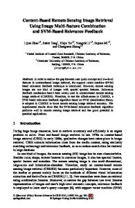
with the Fk-NN and FPARR classification methods. However a better crisp and homogeneous behavior is observed in the WF based classification method compared to the original spectral feature only. This improvement is still better in case of FPARR and further enhanced in case of WF based FPARR based classification methods which can be seen from Figs. 10a and 10b, respectively. The classified images obtained from the WF based ML, k-NN, FML and FE and individual classifiers (original spectral features only) for all wavelets are not shown in figures. However their β values are shown in Tables 3 and 4. Thus it can be summarized that the two classified images in Figs. 9a and 9b showed some visual differences and this difference are still more clear in case of FPARR and WF based FPARR classification methods which are shown in Figs. 10a and 10b, respectively. However a proper comparison can be made from β value, which supports the classification results. Tables 3 and 4 depict the β values for different classification methods. β for the Bombay image with training data is found to be 21.4783, which is 16.8967, 16.8421, 19.4531, 17.6283, 17.0287 and 17.0013 for the ML, k-NN, FPARR, FE, FML and FkNN classifiers, respectively. The β value increment for WF based classifiers in all cases are observed from Tables 3 and 4. It is seen that the same relation on β values are maintained for IRS-1A Bombay image as in the case of Calcutta image. 5.4 Classification of SPOT Calcutta image In case of SPOT Calcutta image, the classified images are shown in Fig. 11a for Fk-NN (original spectral feature only) and Fig. 11b for the WF based FkNN classifiers with Bior3.3 wavelet only. Similarly the classified images with

28

S.K Meher et al. Howrah bridge

Garden reach lake

(a)

Khidirpore dock

Talis nala

Beleghata canal

Race course

(b)

Fig. 11. Classified SPOT Calcutta image by (a) Fk-NN, and (b) WT (Bior3.3) + Fk-NN classification method Howrah bridge

Garden Reach Lake

(a)

Khidirpore Dock

Talis Nala

Beleghata canal

Race Course

(b)

Fig. 12. Classified SPOT Calcutta image by (a) FPARR, and (b) WT (Bior3.3) + FPARR classification method

FPARR and its WF based classification with Bior3.3 wavelet are shown in Figs. 12a and 12b, respectively. From the figures it is observed that there is a clear separation of different classes and some known regions like race course, Howrah Setu(Bridge), Talis nala(Canal), Beleghata canal, Khiderpore dock and Garden Reach Lake. WF based classifier is clearly identifying (Fig. 11b) the above regions compared to those generated by Fk-NN only (Fig. 11a). As in case of IRS-1A Calcutta and Bombay images, here also the identification of


29

different known regions in the classified images are more distinct with FPARR and its WF based classification methods. However, a better performance comparison with the help of β value can be seen from Tables 3 and 4. The β value for the training data set is 9.3343. Its values are 6.8712, 6.8789, 8.1078, 7.0137, 6.9456 and 6.9212 for the ML, k-NN, FPARR, FE, FML and Fk-NN classifiers, respectively. In this case also the improved performance of the WF based classifiers over their original versions are observed and is still better with Bior3.3 wavelet based classification schemes. The β relation in the classification of SPOT Calcutta image is also seen to corroborated the case of IRS-1A Calcutta and IRS-1A Bombay images. From the land cover classification of three remote sensing images, we found that the WF based classification method is superior compared to the corresponding individual classification methods (original spectral feature only). Performance comparison among the six classifiers with its WF based version have been made using a quantitative index (QI). The value of QI supports the superiority of the proposed WF based classification methods over the individual original feature based methods. It is also seen that the Bior3.3 wavelet based classification method is outperforming the other wavelets. Further the improvement of performance with Bior3.3 wavelet and FPARR and FE based classification methods are more prominent, where the β value is close to the training data set compared to the other combination methods. Thus, it is justified that the classified regions using the WF based classification scheme are more crisp and homogeneous compared to their respective original versions as tested in the present case.

6 Conclusion In the present chapter we showed an application of soft computing to remotely sensed image classification. We discussed a wavelet feature based classification approach for land cover classification of multispectral remotely sensed images. The scheme basically tried to explore the possible advantages of using WT as a preprocessor for both non-fuzzy and fuzzy classifiers. In this experiment, we have used two non-fuzzy and four fuzzy classifiers for the performance evaluation. The WT in this case is used to extract features from the original patterns. The extracted features acquire contextual information both in spatial and spectral domains and thus increases classification accuracy. We have used a two-level decomposition of WT, as complexity increases proportionally with the level of decomposition and with an insignificant increase in performance. The improvement in performance of the WF based classification scheme is verified from the results obtained from three remote sensing images. The β measure provide the classification accuracy as shown in Tables 3 and 4. Further, different wavelets are being used in the preprocessing stage of the proposed scheme. Classification results are provided for four wavelets from

30

S.K Meher et al.

two wavelet groups (namely, Daubechies and Biorthogonal). It is observed that WF based approach provided better classification results than any of the corresponding individual classification methods for these remote sensing images. Among the different wavelets, the Bior3.3 wavelet performed better than others. It is observed that the β value for the WF based FPARR and FE classification with Bior3.3 wavelet is close to that of the training data set compared to the others for all the three remote sensing images. Thus, the performance of the FPARR and FE methods convey the information of classification efficiency of fuzzy methods over other methods for these remote sensing images. Hence, it can be concluded that the WF based classification scheme with Bior3.3 wavelet is superior than others in classifying the aforementioned remote sensing images. The present scheme of classification of land covers in remotely sensed imagery can be compared with M-band wavelets [70]; and a comparative study of the wavelet feature based methods with statistical feature (obtained from the gray level co-occurrence matrices) based methods may also be carried out. Other quantitative measures for evaluating the goodness of the classifiers may also be tried. Effectiveness of wavelet features will be tested using other classifiers like neural networks and support vector machines.

Acknowledgements The authors would like to thank the reviewers for their valuable and constructive suggestions. Thanks are also due to the Department of Science and Technology, Government of India and University of Trento, Italy, the sponsors of the India - Trento Program on Advanced Research (Ref: ITALY/ITPAR (IITB, ISI, JU)/2003 dated 22/01/2004), under which a project titled “Advanced Techniques for Remote Sensing Image Processing” is being carried out at the Machine Intelligence Unit, Indian Statistical Institute, Calcutta.

References 1. Tso B., Mather P. M (2001) Classification Methods for Remotely Sensed Data. Taylor and Francis, London 2. Chang C.-I. (2001) Hyperspectral Imaging: Techniques for Spectral Detection and Classification. Kluwer Academic Publishers 3. Varshney P. K., Arora M. K. (2004) Advanced Image Processing Techniques for Remote Sensed Hyperspectral Data. Springer-Verlag, Germany 4. Haralick R. M., Shanmugam K., Dinstein I. (1973) Texture features for image classification. IEEE Transactions on Systems, Man and Cybernetics, 8(6), pp. 610–621 5. Tuominen S., Pekkarinen. A (2005) Performance of different spectral and textural aerial photograph features in multi-source forest inventory. Remote Sensing of Environment, 94(2), pp. 256–268


31

6. Cross G. R., Jain A. K. (1983) Markov random field texture models. IEEE Transactions on Pattern Analysis and Machine Intelligence, 5(1), pp. 25–39 7. Chellappa R., Chatterjee S. (1986) Classification of textures using gaussian markov random fields. IEEE Transaction on Acoustics Speech Signal Processing, 33(4), pp. 959–963 8. Cohen F. S., Fan Z., Patel M. A. (1991) Classification of rotation and scaled textured images using gaussian markov random field models. IEEE Transactions on Pattern Analysis and Machine Intelligence, 13(2), pp. 192–202 9. Derin H., Elliot H. (1987) Modeling and segmentation of noisy and textured images using gibbs random fields. IEEE Transactions on Pattern Analysis and Machine Intelligence, 9(1), pp. 39–55 10. Unser M. (1986) Local linear transforms for texture measurements. Signal Processing, 11, pp. 61–79 11. Unser M. (1995) Texture classification and segmentation using wavelet frames. IEEE Transactions on Image Processing, 4(11), pp. 1549–1560 12. Park S. C., Park M. K., Kang M. G. (2003) Super-resolution image reconstruction: a technical overview. IEEE Signal Processing Magazine, 20(3), pp. 21–36 13. Ng M. K., Bose N. K. (2003) Mathematical analysis of super-resolution methodology. IEEE Signal Processing Magazine, 20(3), pp. 62–74 14. Rajan D., Chaudhuri S., Joshi M. V. (2003) Multi-objective super resolution: concepts and examples. IEEE Signal Processing Magazine, 20(3), pp. 49–61 15. Keshava N., Mustard J. F. (2002) Spectral unmixing. IEEE, Signal Processing Magazine, 19(1), pp. 44–57. 16. Brown M., Gunn S. R., Lewis H. G. (1999) Support vector machines for optimal classification and spectral unmixing. Ecological Modelling, 120, pp. 167–179 17. Chang C. I., Ren H. (2000) An experiment-based quantitative and comparative analysis of target detection and image classification algorithms for hyperspectral imagery. IEEE Transactions on Geoscience and Remote Sensing, 38(2), pp. 1044–1063 18. Faraklioti M., Petrou M. (2001) Illumination invariant unmixing of sets of mixed pixels. IEEE Transactions on Geoscience and Remote Sensing, 39(10), pp. 2227–2234 19. Shah C. A., Varshney P. K. (2004) A higher order statistical approach to spectral unmixing of remote sensing imagery. Proceedings of the IEEE International Symposium on Geoscience and Remote Sensing, volume 39, pp. 1065–1068 20. Parra L., Mueller K. R., Spence C., Ziehe A., Sajda P. (2000) Unmixing hyperspectral data. Advances in Neural Information Processing Systems, volume 12, MIT Press 21. Robila S. A. (2002) Independent component analysis feature extraction for hyperspectral images. PhD thesis, EECS Department. Syracuse University, Syracuse, NY 22. Chang C. I., Chiang S.-S., Smith J. A., Ginsberg I. W. (2002) Linear spectral random mixture analysis for hyperspectral imagery. IEEE Transactions on Geoscience and Remote Sensing, 40(2), pp. 375–392 23. Burke D. P., Kelly S. P., Chazal P. de, Reilly R. B., Finucane C. (2005) A parametric feature extraction and classification strategy for brain-computer interfacing. IEEE Transactions on Neural Systems and Rehabilitation Engineering, 13(1), pp. 12–17

32

S.K Meher et al.

24. Song C. (2005) Spectral mixture analysis for subpixel vegetation fractions in the urban environment How to incorporate endmember variability? Remote Sensing of Environment, 95, pp. 248–263 25. Plaza A., Martinez P., Perez R., Plaza J. (2002) Spatial/spectral endmember extraction by multidimensional morphological operations. IEEE Transactions on Geoscience and Remote Sensing, 40(9), pp. 2025–2041 26. Barducci A., Mecocci A., Alamanno C., Pippi I., Marcoionni P. (2003) Multiresolution least-squares spectral unmixing algorithm for subpixel classification of hyperspectral images. Proceedings of the IEEE International Symposium on Geoscience and Remote Sensing, volume 3, pp. 1799–1801 27. Broadwater J., Meth R., Chellappa R. (2004) A hybrid algorithm for subpixel detection in hyperspectral imagery. Proceedings of the IEEE International Symposium on Geoscience and Remote Sensing, volume 3, pp. 1601–1604 28. Tatem A. J., Lewisa H. G., Atkinsonb P. M., Nixona M. S. (2002) Superresolution land cover pattern prediction using a hopfield neural network. Remote Sensing of Environment, 79, pp. 1–14 29. Weiguo L., Seto K. C., Wu E. Y., Gopal S., Woodcock C. E. (2004) ART-MMAP: A neural network approach to subpixel classification. IEEE Transactions on Geoscience and Remote Sensing, 42(9), pp. 1976–1983 30. Pastina D., Farina A., Gunning J., Lombardo P. (1998) Classification of rotation and scaled textured images using gaussian markov random field models. IEE Proceedings Radar, Sonar Navigation, 145(5), pp. 281–290 31. Jiang N., Wu R., Li J. (2001) Super resolution feature extraction of moving targets. IEEE transactions on Aerospace and Electronic Systems, 37(3), pp. 781–793 32. Foody G. M., Muslim A. M., Atkinson P. M. (2003) Super-resolution mapping of the shoreline through soft classification analyses. Proceedings of the IEEE International Symposium on Geoscience and Remote Sensing, volume 6, pp. 3429–3431 33. Qing K., Yu R., Li X., Deng X. (2005) Application of spectral angle mapping model to rapid assessment of soil salinization in arid area. Proceedings of the IEEE International Symposium on Geoscience and Remote Sensing, volume 4, pp. 2355–2357 34. Shih E. H. H., Schowengerdt R. A. (1983) Classification of arid geomorphic surfaces using spectral and textural features. Photogrammetric Engineeing and Remote Sensing, 49(3), pp. 337–347, 1983 35. Yuan X., King D., Vlcek J. (1991) Sugar maple decline assessment based on spectral and textural analysis of multispectral aerial videography. Remote Sensing of Environment, 37(1), pp. 47–54 36. Chica-Olmo M., Abarca-Hern´ andez F. (2000) Computing geostatistical image texture for remotely sensed data classification. Computers and Geosciences, 26(4), pp. 373–383 37. Jouan A., Allard Y. (2004) Land use mapping with evidential fusion of features extracted from polarimetric synthetic aperture radar and hyperspectral imagery. Information Fusion, 5(4), pp. 251–267 38. Mallat S. (1999) A Wavelet Tour of Signal Processing. Academic Press, 2nd edition 39. Strang G., Nguyen T. (1996) Wavelets and Filter Banks. Wellesley College


33

40. Chang T., Kuo C. C. J. (1993) Texture analysis and classification with treestructured wavelet transform. IEEE Transactions on Image Processing, 2(4), pp. 429–440 41. Unser M., Eden M. (1989) Multiresolution feature extraction and selection for texture segmentation. IEEE Transactions on Pattern Analysis Machine Intelligence, 2, pp. 717–728 42. De Wouwer G. V., Schenders P., Dyek D. V. (1999) Statistical texture characterization from discrete wavelet representation. IEEE Transactions on Image Processing, 8(4), pp. 592–598 43. Abbate A., Das P., Decusatis C. M. (2001) Wavelets and Subbands: Fundamentals and Applications. Springer 44. Arivazhagan S., Ganesan L. (2003) Texture classification using wavelet transform. Pattern Recognition Letters, 24, pp. 1513–1521 45. Szu H. H., Moigne J. L., Netanyahu N. S., Hsu C. C. (1997) Integration of local texture information in the automatic classification of landsat images. SPIE Proceedings, 3078, pp. 116–127 46. Yu J., Ekstrom M. (2003) Multispectral image classification using wavelets: A simulation study. Pattern Recognition, 36, pp. 889–898 47. Alpert B. K. (1992) Wavelets and other bases for fast numerical linear algebra. In Wavelets: A Tutorial in Theory and Applications, C. K. Chui, Ed. New York: Academic Press, pp. 181–216 48. Strela V., Heller P. N., Strang G., Topiwala P., Heil C. (1999) The application of multiwavelet filter banks to image processing. IEEE Transactions on Image Processing, 8(4), pp. 548–563 49. Soltanian-Zadeh H., Rafiee-Rad F., Pourabdollah-Nejad D. S. (2004) Comparison of multiwavelet, wavelet, haralick, and shape features for microcalcification classification in mammograms. Pattern Recognition, 37, pp. 1973–1986 50. Duda R. O., Hart P. E., Stork D. G. (2000) Pattern Classification. Wiley Interscience Publications, 2nd edition 51. Pedrycz W. (1990) Fuzzy sets in pattern recognition: methodology and methods. Pattern Recognition, 23(1/2), pp. 121–146 52. Kuncheva L. I. (2000) Fuzzy Classifier Design. Springer-Verlag 53. Cover T. M., Hart P. E. (1967) Nearest neighbor pattern classification. IEEE Transactions on Information Theory, 13(1), pp. 21–27 54. Wang F. (1990) Fuzzy supervised classification of remote sensing images. IEEE Transactions on Geoscience and Remote Sensing, 28(2), pp. 194–201 55. Keller J. M., Gray M. R., Givens J. A. (1985) A fuzzy k-nearest neighbor algorithm. IEEE Transactions on Systems, Man and Cybernetics, 15(4), pp. 580–585 56. Ghosh A., Meher S. K., Shankar B. U. (2005) Fuzzy supervised classification using aggregation of features. Technical Report, Indian Statistical Institute. No. MIU/TR-02/2005 57. Melgani F., AI Hashemy B. A. R., Taha S. M. R. (2000) An explicit fuzzy supervised classification method for multispectral remote sensing images. IEEE Transactions on Geoscience and Remote Sensing, 38(1), pp. 287–295 58. Richards J. A., Jia X. (1999) Remote Sensing Digital Image Analysis: An Introduction. New York: Springer Verlag, 3rd edition 59. Daubechies I. (1995) Ten Lectures on Wavelets. Society for Industrial and Applied Mathematics 60. Liu H., Motoda H. (1998) Feature Extraction, Construction and Selection: A Data Mining Perspective. Kluwer Academic Publishers, Norwell, MA, USA

34

S.K Meher et al.

61. Mazzaferri J., Ledesma S., Iemmi C. (2003) Multiple feature extraction by using simultaneous wavelet transforms. Journal of Optics, A Pure and Applied Physics, 5, pp. 425–431 62. Soltani S., Simard P., Boichu D. (2004) Estimation of the self-similarity parameter using the wavelet transform. Signal Processing, 84(1), pp. 117–123 63. Mujica F. A., Leduc J. P., Murenzi R., Smith M. J. T. (2000) A new motion parameter estimation algorithm based on the continuous wavelet transform. IEEE Transactions on Image Processing, 9(5), pp. 873–888 64. Topiwala P. K. (2000) Wavelet Image and Video Compression. Springer 65. Vetterli M., Kovacevic J. (1995) Wavelets and Subband Coding. Prentice Hall, 1st edition 66. Chen C. F. (1999) Fuzzy training data for fuzzy supervised classification of remotely sensed images. Asian Conference on Remote Sening (ACRS 1999) 67. Zadeh L. A. (1965) Fuzzy sets. Information Control, 8, pp. 338–353 68. Cohen J. (1960) A coefficient of aggrement for nominal scale. Education and psychological measurement, 20(1), pp. 37–46 69. Pal S. K., Ghosh A., Shankar B. U. (2000) Segmentation of remotely sensed images with fuzzy thresholding, and quatitative evaluation. International Jounal of Remote Sensing, 21(11), pp. 2269–2300 70. Acharyya M., De R. K., Kundu M. K. (2003) Segmentation of remotely sensed images using wavelet features and their evaluation in soft computing framework. IEEE Transactions on Geoscience and Remote Sensing, 41(12), pp. 2900–2905 71. Mitra P., Shankar B. U., Pal S. K. (2004) Segmentation of multispectral remote sensing images using active support vector machines. Pattern Recognition Letters, 25(12), pp. 1067–1074 72. IRS data users hand book (1989) Technical Report. Document No. IRS/NRSA/NDC/HB-02/89