Keywords: Multistability; chaos; basin boundaries; suspension bridge. 1. Introduction ..... tonian case there is an infinite number of periodic orbits, we find only a ...
Papers International Journal of Bifurcation and Chaos, Vol. 14, No. 3 (2004) 927–950 c World Scientific Publishing Company
MULTISTABILITY, BASIN BOUNDARY STRUCTURE, AND CHAOTIC BEHAVIOR IN A SUSPENSION BRIDGE MODEL ´ MARIO S. T. DE FREITAS∗ and RICARDO L. VIANA Departamento de F´ısica, Universidade Federal do Paran´ a, C.P. 19081, 81531-990, Curitiba, Paran´ a, Brazil CELSO GREBOGI Instituto de F´ısica, Universidade de S˜ ao Paulo, C.P. 66318, 05315-970, S˜ ao Paulo, SP, Brazil Received July 3, 2002; Revised October 16, 2002 We consider the dynamics of the first vibrational mode of a suspension bridge, resulting from the coupling between its roadbed (elastic beam) and the hangers, supposed to be one-sided springs which respond only to stretching. The external forcing is due to time-periodic vortices produced by impinging wind on the bridge structure. We have studied some relevant dynamical phenomena in such a system, like periodic and quasiperiodic responses, chaotic motion, and boundary crises. In the weak dissipative limit the dynamics is mainly multistable, presenting a variety of coexisting attractors, both periodic and chaotic, with a highly involved basin of attraction structure. Keywords: Multistability; chaos; basin boundaries; suspension bridge.
ment, like that encountered in the Tacoma Narrows bridge failure [Lazer & McKenna, 1990]. The possible inadequacy of a linear explanation for this disaster has been already questioned by the board of experts, including von K´arm´an himself, that have produced a report to the U.S. Federal Works Agency [Amann et al., 1941]. Nowadays the role of nonlinear effects in the Tacoma Narrows disaster (as well as of other similar suspension bridges) has been widely accepted. Two aspects of the problem have been pointed out: firstly, the Tacoma Narrows Bridge was originally built with a slender, light and flexible roadbed. As a result, large-amplitude transversal oscillations were possible under widely different wind conditions. Secondly, as can be seen in the famous movie shot at
1. Introduction A well-known and quite dramatic example of the resonance effects on structures under the action of time-periodic forcing is the Tacoma Narrows bridge failure, that occurred on 7 November, 1940 [Amann et al., 1941]. The source of an external driving force is the aeolian harp effect caused by a periodic force generated by a von K´arm´an street of staggered vortices due to impinging wind on the bridge structure [Blevins, 1977]. However, the standard textbook explanation based on the linear resonance between the frequency of the vortex street and the bridge natural frequency has been recently questioned by many authors [Billah & Scanlan, 1991]. Basically, linear resonance is a rather narrow phenomenon, unlikely to occur in an irregularly changing environ∗
Permanent address: Departamento de F´ısica, Centro Federal de Educa¸cao Tecnol´ ogica do Paran´ a, Curitiba, PR, Brazil. 927
928
M. S. T. de Freitas et al.
the moment of disaster,1 torsional oscillations were also observed just before the bridge collapsed [Lazer & McKenna, 1990]. Coupling between such different modes is a typical nonlinear feature [Nayfeh & Mook, 1979]. The torsional mode is particularly sensitive to the nonlinearly elastic nature of the hangers that connect the roadbed to the main suspension cable. A key point to explain the suspension bridge collapse is that, in this and other related situations, a nonlinear response can lead to various complex dynamical phenomena, such as different modes of vibration, traveling waves and chaotic motion. Nonlinearity appears in a rather robust way in suspension bridges, since the myriad of cables that connect the roadbed to the main suspended cable have a peculiar characteristic: a cable strongly resists to stretching but does not to compression. This leads to a piecewise linear stiffness for the cables, and the oscillator dynamics is governed by a nonsmooth linear vector field, with many features common to nonlinear systems [Blazejczyk-Okulewska et al., 1999]. The piecewise linear stiffness found in the oscillations of a suspension bridge is just one of the various examples of mechanical systems with discontinuities [Wiercigroch & DeKraker, 2000]. Related examples of technological interest are impact oscillations due to clearances or gaps between moving parts like rotors and their bearings or shafts [Aidanpaa et al., 1994; Wiercigroch, 2000; Blazejczyk-Okulewska, 2000; Jerrelind & Stensson, 2000], and stick-slip vibrations [Popp & Stelter, 1990]. This has motivated many analytical and numerical studies on such oscillators, as the seminal paper of Shaw and Holmes [1983] on the bilinear oscillator, and the ensuing work by Thompson et al. [1983], Whiston [1987], Nordmark [1991], and Kim and Noah [1991], among many others. In a model proposed by Lazer and McKenna in the early 90’s [Lazer & McKenna, 1990], a suspension bridge deck is assumed to be a one-dimensional elastic beam connected to the main suspended cable by a large number of hangers, treated as onesided springs. According to the behavior displayed by the Tacoma Narrows bridge just before its failure, the first transversal harmonic was the domi-
nant one and it resulted in a vibration amplitude of 1.5 ft, excited by 35 mph winds. After three hours, the wind increased to 42 mph and the growing oscillation amplitude caused a hanger to escape out of its roadbed connection, resulting in an unbalanced loading and to a 0.2 Hz torsional vibration model which ultimately caused the bridge to collapse. 2 Instead of solving a boundary value problem for the partial differential equation describing the full spatio-temporal problem [Heertjes & Van de Molengraft, 2001], the strategy of [Lazer & McKenna, 1990] was to isolate and analyze the time evolution of the first vibrational mode alone, by means of an initial value problem for an ordinary differential equation. The Lazer–McKenna model was further investigated by Doole and Hogan [1996], who have considered the periodic response of the bridge to variations of the external driving parameters, in which the action of the vortex trail on the structure was modeled by a periodic force. Another feature investigated was the role of the preload caused by the proper weight of the roadbed. In a later work, this analysis was extended to the torsional vibration modes of the bridge [Doole & Hogan, 2000]. In this work, we do not restrict ourselves to periodic behavior of the bridge [Doole & Hogan, 1996], but we consider the more complex behavior expected in a nonlinear system. We explore a wide region of the forcing-damping parameter space, for which we find periodic, quasiperiodic and chaotic behavior. Moreover, for weak dissipation we observe a predominance of multistable behavior, involving both periodic and chaotic attractors, with a highly convoluted basin of attraction structure. In spite of this, the basin boundaries are not necessarily fractal curves, as it typically happens in driven oscillators. Abrupt changes of chaotic behavior also occurs for this system and they are related to boundary crises. The rest of this paper is organized as follows: in the second section, we outline the dynamical model of the first vibrational mode of a suspension bridge as a piecewise-linear driven and damped one-dimensional oscillator, following [Lazer & McKenna, 1990] and [Doole & Hogan, 1996]. Section 3 considers the harmonic, or periodic, response
1 Images of the Tacoma Narrows bridge disaster are available on the website http://cee.carleton.ca/Exhibits/TacomaNarrows/, taken from the 20-minute silent movie. 2 See the website http://www.vibrationdata.com/Tacoma.htm for details.
Multistability and Chaos in a Suspension Bridge
of the undamped oscillator. The fourth section is devoted to the analysis of the multistable periodic behavior observed for wide regions of the forcingdamping parameter space. The basin boundary structure is considered in Sec. 5, whereas Sec. 6 analyzes the onset of chaotic behavior and abrupt changes in the chaotic attractors due to a boundary crises. The last section contains our conclusions.
929
Fig. 1. Schematic figure of a suspension bridge. The hangers connect an elastic beam representing the bridge deck to the main suspension cable.
2. Suspension Bridge Model The deck, or roadbed, of a suspension bridge is assumed to be an elastic vibrating beam sustained by hangers, which are steel cables attached to a main suspended cable (Fig. 1). The elastic beam is hinged at both ends to an anchorage block, and the main cable is supported by high towers. We shall consider a simplified model of a suspension bridge which takes into account only the elasticity of its deck and of the hangers that support it. We neglect deflections of the main suspended cable and other structural components. We use x and z as the longitudinal and transversal coordinates of the vibrating beam, respectively, whereas u is the beam deflection along y (Fig. 1), assuming a downward deflection as positive (u > 0). In this paper we consider only the transversal beam vibrations so that we ignore the influence of the transverse coordinate z. Hence, the beam deflection is taken to be only a function of the longitudinal coordinate and the time, i.e. u = u(x, t). The hangers are assumed as being one-sided strings: they do not withstand compression efforts, but they oppose a linear restoring force when stretched, provided the deformations are small enough to be treated in the elastic regime [Lazer & McKenna, 1990]. Hence, the stiffness response of a hanger is piecewise linear and asymmetric, this nonlinear response being the source of the complex dynamical behavior in the system. The elastic restoring force offered by the hangers can be expressed as −k 0 u+ , where k 0 is the spring constant and u+ = max{u, 0}. In this case, the elastic response of the bridge has two distinct features: for downward deflections, we take into account the combined response of the beam and stretched hangers, whereas, for upward deflections, only the beam elasticity is considered. Moreover, we add a preloading term W (x) in the bridge model, due to the proper beam weight and
its loading. The partial differential equation governing the beam vibration is [Hartog & Pieter, 1987] M
∂2u ∂4u ∂u + EI + δ0 2 4 ∂t ∂x ∂t = −k 0 u+ + W (x) + F (x, t) ,
(1)
where M is the beam mass per unit length, E is the Young modulus of the beam, and I the moment of inertia of its transversal section. The dissipative effect on the beam vibration is modeled by a viscous damping term δ 0 ut . The external force F (x, t) represents the periodic driving effect of a Von Karman vortex street. If the wind incidence is along the transversal direction z, the external force is collinear to the deflection with a well-defined period T = 2π/ω 0 F (x, t) = F0 (x) sin(ω 0 t) .
(2)
The boundary conditions for Eq. (1) take into account the hinging of the beam at its ends (x = 0 and x = L): ∂ 2 u ∂ 2 u = = 0 . (3) u(0, t) = u(L, t) = ∂x2 (0,t) ∂x2 (L,t)
Instead of solving (1) directly, we will consider the time evolution of the bridge transversal vibrating modes. In particular, only the first transversal harmonic is to be considered in this work (Fig. 2). Besides being the most commonly observed mode for low velocities in the Tacoma Narrows Bridge [Amann et al., 1941], the loss of stability of this mode was responsible for the torsional oscillations that eventually led to its failure [Billah, 1991]. This assumption implies that the preloading and the spatial part of the external force can be written, respectively, as � πx � � πx � , F0 (x) = B 0 sin . (4) W (x) = W 0 sin L L
930
M. S. T. de Freitas et al.
by the following ordinary differential equation � π �4 d2 y dy M 2 + δ0 y + k0 y+ + EI dt dt L = W 0 + B 0 sin(ω 0 t) .
Fig. 2. First transversal vibration mode of the beam representing the suspension bridge roadbed.
Since the preloading W is usually taken to be a constant value, the decomposition for W (x), Eq. (4), should be intended as the first term in the harmonic expansion of a constant function. The relative error in taking only the lowest order is less than 10% in the deflections [Lazer & McKenna, 1990]. In the same spirit, we separate the independent variables in the beam deflection as � πx � u(x, t) = y(t) sin , (5) L where y(t) = u(L/2, t) indicates the deflection of the bridge roadbed at its midpoint, assuming positive (negative) values of y(t) for downward (upward) deflections, and with time evolution governed
(a)
(6)
We introduce nondimensional spatial and temporal variables as follows � π �2 r EI πx ˆ x ˆ= , t= t, (7) L L M as well as the normalized parameters � �4 0 � �2 δ0 L k L √ , k= δ= , (8) π π EI 2 EIM � �2 r � �4 0 B M L L 0 ω ω= , B= , π EI π EI (9) � �4 L W0 , W = π EI such that Eq. (6) is rewritten as y 00 + 2δy 0 + my = W + B sin(ωt) ,
(10)
where the primes denote derivatives with respect to the scaled time, the hats on the variables were removed for ease of notation, and � 1 if y < 0, (11) m= (k + 1) if y > 0,
(b)
Fig. 3. One-dimensional oscillator with two springs, one of them with a clearance, equivalent to the suspension bridge flexional vibrations. (a) Upward deflections, for which only the beam stiffness is acting; (b) downward deflections, for which both the beam and hanger stiffnesses occur. The string in the upper part of the figure plays no role in the elastic response of the oscillator.
Multistability and Chaos in a Suspension Bridge
represents the slopes of the two pieces of the response curve. Driven piecewise linear oscillators have been extensively studied in the literature [Shaw & Holmes, 1983; Thompson et al., 1983; Whiston, 1987; Nordmark, 1991], but in Eq. (10) the presence of the preload W leads to some essential differences with the already known cases. Figure 3 shows a mechanical oscillator equivalent to Eq. (10), in which there are two springs with stiffness constants equal to 1 and k, respectively. Whereas the first spring is always connected to the vibrating mass, the second spring has a clearance with respect to it. This kind of oscillator has many applications in the impact vibration literature [Wiercigroch, 2000]. The nonsmoothness of the vector field (10) at y = 0 preserves the Lifshitz property, and thus the existence and uniqueness theorem for differential equations still holds [Guckenheimer & Holmes, 1983]. However, while many standard results of
931
dynamical system theory remain applicable for this type of systems, some important ones do not. For example, standard bifurcation theory does not apply [Chin et al., 1994], as well as most techniques for computing Lyapunov exponents [Kapitaniak, 2000].
3. Periodic Orbits in the Undamped Bridge Dynamics Let us first consider that both the damping and the external force vanish (δ = 0, B = 0). In this case the suspension bridge model (10), governing the deflections of the first vibrational mode, can be written in the form y 00 = Feff (y) = −dVeff (y)/dy, where Veff (y) = −W y +
1 my 2 2
(12)
is an effective potential which contains the effects of the piecewise linear stiffness and the constant preload.
(a)
(b)
(c)
(d)
(e)
(f)
Fig. 4. Restoring force (solid line) and the corresponding effective potential (dashed line) as a function of the vertical bridge deflection y, without preload: (a) hanger stiffness; (b) beam stiffness; (c) combined stiffness. (d)–(f) Same cases, but with preload.
932
M. S. T. de Freitas et al.
Figures 4(a)–4(c) show both the effective force and potential for the hangers, beam and the combined system respectively, without preload (W = 0). The hangers act as one-sided springs, according to Eq. (4), whereas the beam experiences a linear restoring force, such that the effective potential for the combined system is an asymmetric curve. The existence of a preload (W 6= 0) causes the appearance of a small harmonic well at the bottom of the effective potential curve, as can be seen in Figs. 4(d)–4(f). Small amplitude oscillations (called preloaded orbits by Doole and Hogan [1996]) are strictly linear and can be analytically solved [Nayfeh & Mook, 1979]. We are, however, interested in the large amplitude oscillations, for which the nonsmoothness of the effective potential plays a key role, and which requires a numerical solution of Eq. (10), although approximate analytical methods can be used to treat some particular cases [Kim & Noah, 1991; Cao et al., 2001]. Accordingly, we have numerically solved (10) by using a 12th order Adams method (from the LSODA package [Hindmarch, 1983]). In Fig. 5 we depict a typical phase portrait (downward displacement versus downward velocity of the bridge) for the free and undamped case. The three preloaded orbits shown are harmonic smallamplitude oscillations encircling the stable equilibrium point located at y = y0 = W/(k + 1) and y˙ = 0. Large amplitude bridge oscillations, on the other hand, are closed curves formed by arcs of ellipses for y > 0 smoothly joined to arcs of circles for y < 0. Points for which y = 0 form a line of nonsmoothness of the vector field (10), or a switching manifold, using the terminology of DiBernardo et al. [2001]. While the free and undamped case has an integrable (in the Liouville sense) Hamiltonian Hu (p, y) = 12 p2 + Veff (y) = const. (where p = y 0 is the momentum conjugate to the downward bridge deflection y), the driven case is nonintegrable due to the explicit time-dependence present in the forcing term of the Hamiltonian Hf (p, y, t) =
1 2 1 p + my 2 − W y − By sin(ωt) . 2 2 (13)
The effect of the preload can be absorbed into the above Hamiltonian by making a shift of the origin from y = 0 to the equilibrium at y = y0 , by means of a canonical transformation (p, y, t) → (p z , z, t)
Fig. 5. Trajectories in the phase plane (y1 = y, y2 = y) ˙ for the undamped and free bridge oscillations, with k = 10 and W = 1, corresponding to six different initial conditions. Preloaded orbits have all their points with y > 0.
using the generating function � � W F2 (pz , y, t) = (y − y0 )pz = y − pz , (14) 1+k such that the new Hamiltonian is, up to an unessential constant, equal to 1 1 1 H f (pz , z, t) = p2z + z 2 − kΘ(y)z 2 2 2 2 � � W −B z+ sin(ωt) , (15) 1+k where we have written for the nonsmooth elastic function m the expression m(y) = 1 + kΘ(y) ,
(16)
in which Θ(y) is the unit step function. We can formally treat the time dependence by passing to an extended phase space, by setting t ≡ τ as an additional coordinate, and with E = −H f as its conjugate momentum [Lichtenberg & Lieberman, 1997]. An auxiliary parameter ξ can be chosen to play the role of time in this case. The Hamiltonian of the forced system in the extended phase space is 1 1 1 He (pz , E; z, τ ) = p2z + z 2 + E + kΘ(z(y))z 2 2 2 2 � � W −B z+ sin(ωτ ) 1+k =E, (17)
Multistability and Chaos in a Suspension Bridge
and dynamically similar to an autonomous twodegree-of-freedom system. It is non-integrable for there is no other independent integral of motion besides E. In the above expression, the two first terms refer to a simple harmonic oscillator, for which we can introduce the corresponding action and angle variables (J, θ), defined as [Lichtenberg & Lieberman, 1997] √ √ (18) z = 2J sin θ , pz = 2J cos θ , in such a way that (17) reads H(J, E; θ, τ ) =J +E +kΘ(y(J, θ))J sin2 θ � � √ W 2J sin θ+ −B sin(ωτ ) . 1+k (19) We complete the algebra by making a second canonical transformation to the action and angle variables related to the energy-time pair (J ϑ , Jϕ ; ϑ, ϕ), using the generating function F˜2 (Jϑ , Jϕ ; θ, τ ) = ωτ Jϕ + θJϑ , such that the Hamiltonian is H(Jϑ , Jϕ ; ϑ, ϕ) = H0 (Jϑ , Jϕ ) + H1 (Jϑ , Jϕ ; ϑ, ϕ) = Jϑ + ωJϕ + kΘ(y(Jϑ , ϑ))Jϑ sin2 ϑ �p � W − B sin ϕ 2Jϑ sin ϑ + . (20) 1+k The (extended) phase space for the forced oscillator has four dimensions, but the energy surface (on which the system trajectories lie) is only threedimensional, since E = E(Jϑ , Jϕ ; ϑ, ϕ) = const. and there are only three independent variables, one of them being the angle ϕ = ϕ0 + ωt, mod 2π. Thus we can study the system using a Poincar´e surface of section constructed at ϕ = 0, which is equivalent to a stroboscopic time-T map, where T = 2π/ω. The two angle variables (ϑ and ϕ) characterize the foliation of the phase space into nested closed surfaces with the topology of tori. Closed curves in a Poincar´e surface of section are thus intersections of invariant tori. We define two frequencies related to each angle parameterizing the dynamics on these tori, defined in terms of the unperturbed part of the Hamiltonian (20), as follows ωϑ =
∂H0 = 1, ∂Jϑ
ωϕ =
∂H0 = ω, ∂Jϕ
(21)
933
where ωϕ is the frequency of the external forcing, and ωϑ = 1 is the frequency of the closed orbits of the unperturbed harmonic oscillator (H 0 (J) = J). The dynamical response of the forced system depends in a large extent on the ratio between these frequencies, or the winding number α=
1 ωϑ = . ωϕ ω
(22)
If the winding number is a rational number of the form m/n, where m and n are co-prime integers, then the frequencies are commensurate, in that there are integer values of m and n for which mωϕ − nωϑ = 0, or a m : n primary resonance, with the following cases [Wiggins, 1997]: harmonic response (m = n = 1); subharmonic response of order m (m > 1 and n = 1); ultra-harmonic response of order m (m = 1 and n > 1); and ultra-subharmonic response of order m, n (m > 1 and n > 1). A m : n resonance is a trajectory that closes on itself after n complete turns in the long way along the torus (ϕ), and m turns in the short way (ϑ). In terms of the Poincar´e surface of section (J ϑ , ϑ) we thus have m distinct points for a m : n resonance. These are marginally stable periodic orbits for the time-T map, whose eigenvalues are equal to one in absolute value. In the nested tori structure the periodic orbits are arbitrarily close to one another, for m and n can both be large integers. On the other hand, if the winding number α is irrational, a trajectory never closes on itself, and densely fills a torus, represented by closed curves in the Poincar´e section (quasiperiodic response). Consider the example depicted in Fig. 6, where we have relatively weak forcing. We have a 1 : 1 primary resonance located close to the preloaded equilibrium point of the unforced system, as well as resonances with m equal to 4, 3, 7, and 2, in increasing order of relative distance to the 1 : 1 central resonance. The outermost closed curve shown in Fig. 6 represents a quasiperiodic orbit, just like the closed curves encircling the resonances. This is a rather general behavior observed in integrable Hamiltonian systems subjected to a small nonintegrable perturbation [Lichtenberg & Lieberman, 1997]. Canonical perturbation theory fails when applied at resonances due to the divergent terms they cause in the perturbation series. A standard procedure (secular perturbation theory) removes these divergences by using two time scales, and averaging over the fast angle. The structure around a given
934
M. S. T. de Freitas et al.
Fig. 6. Trajectories in the phase plane (y1 = y, y2 = y) ˙ for the undamped and forced bridge oscillations, with B = 0.5, ω = 4.3, k = 10, and W = 1, corresponding to different initial conditions.
primary resonance is topologically similar to a nonlinear pendulum, in the sense that there are “librations”, or closed trajectories which in Fig. 6 encircle the various m : n subharmonic resonances (chain of order-m periodic islands). These islands are formed by quasiperiodic orbits which wind around the torus in the same way as the periodic orbits do. For example, the m = 4 island in Fig. 6 completes four turns in the long way along the torus, before closing on itself. At each intermediate crossing a trajectory visits a different island belonging to the chain, which is roughly delimited by a locally chaotic layer. The island width increases with the square root of the perturbation strength [Lichtenberg & Lieberman, 1997], which is proportional to the amplitude of the external forcing B. Primary islands are, in turn, surrounded by smaller secondary islands corresponding to harmonics between one of the fundamental frequencies and the frequency of the librations inside a primary island, and so on. Figure 7 presents a situation found for higher values of B and k. Differently from the large number of resonances shown in Fig. 6, now only the 2 : 1 one is still visible, what leads us to conclude that other islands were either engulfed or are simply too narrow to be resolved. Besides the quasi-integrable curves encircling the entire system as well as the 2 : 1
Fig. 7. Phase space trajectories for higher forcing amplitude (B = 3.0) and hanger stiffness (k = 50), the remaining parameters being the same as in the preceding figure.
resonance, the noteworthy feature is the existence of a wide area-filling chaotic region. The fact that most nonchaotic trajectories are quasiperiodic is not by chance, being rather predicted by the KAM theory: under a sufficiently small perturbation most irrational tori are preserved, even though with some alteration of their shapes. Chaotic trajectories appear due to heteroclinic intersections of stable and unstable manifolds of the hyperbolic points connecting adjacent islands of a same chain. These trajectories do not lie on invariant tori and, for weak perturbation, form a narrow area-filling layer around a given island. As the island itself is enlarged for stronger perturbation, its chaotic layer similarly increases in width. Chaotic layers belonging to adjacent layers may even fuse and engulf intermediate chains, as the perturbation builds up, as can be observed in Fig. 7. If the perturbation is small enough such that there are surviving quasiperiodic trajectories (KAM tori) between adjacent resonances, the chaotic layers do not allow for large excursions of a chaotic trajectory. For higher perturbation, however, these KAM tori are progressively destroyed and their chaotic layers overlap, generating large scale excursions. There is an extensively studied barrier transition between these two chaotic regimes [Chirikov, 1979]. Even in this case, the wide chaotic region continues to be bounded by KAM surfaces that
Multistability and Chaos in a Suspension Bridge
encircle the overall structure, as shown in Fig. 7. In conclusion, even for higher forcing amplitudes we cannot expect chaotic motion everywhere in the energy surface, but rather a stochastic diffusion of area-filling trajectories over a limited portion of the phase-space.
4. Multistability in the Damped Bridge Dynamics In this section, we consider the effects of adding a small viscous damping in the otherwise conservative system represented by the suspension bridge model. The discussion is based on the properties the system displays in the absence of dissipation, and are related to the periodic, quasiperiodic or chaotic nature of the orbits. Being now a dissipative system,
935
there is no longer an energy surface to work with, but as the system still has a time-periodic variable related to the external forcing, we can also make a Poincar´e section by a stroboscopic, or time-T sampling: (y(t), y(t)) ˙ 7→ fT (y, y) ˙ = (y(t+T ), y(t+T ˙ )). An example of stroboscopic plot of a harmonic response, with nonzero damping and forcing, is shown in Fig. 8, where the different colors represent the basins of attraction of stable orbits with periods equal to 1 (black), 2 (yellow), 3 (red) and 4 (cyan). In Figs. 9(a)–9(c) we present phase portraits, for both continuous and discrete time, for orbits with periods equal to two, three and four, respectively; whereas in Fig. 9(d) the four orbits are shown together. The existence of four observed periodic orbits corresponding to subharmonics of the periodic
Fig. 8. Phase portrait (y − y) ˙ for the stroboscopic (time-T ) map for W = 1, δ = 0.01, k = 10, B = 0.5, and ω = 2π/T = 4.3. We indicate the existence of basins of attraction of multiple coexisting periodic orbits by using colors: period-1 (black), period-2 (yellow), period-3 (red), period-4 (cyan), period-5 (dark green). The central region has a higher resolution than the rest of the figure.
936
M. S. T. de Freitas et al.
(a)
(b)
(c)
(d)
Fig. 9. Trajectories in the phase plane (y, y) ˙ corresponding to coexisting periodic orbits whose basins are depicted in Fig. 8: (a) period-2 (squares); (b) period-3 (diamonds); and (c) period-4 (stars). The marked points are from the corresponding stroboscopic map, and are shown together in (d).
driving term, illustrates multistability in the oscillator response to the external forcing. The general features shown in Fig. 8 are expected for conservative systems with small dissipation, and can be explained in rather general grounds. The island centers, which were marginally stable periodic orbits (sources) of the conservative system, become periodic attractors (sinks or stable foci) for the strobo-
scopic map, whose eigenvalues are smaller than one in absolute value. The periodic orbits in Fig. 8 will be labeled F 1 to F 4. However, while in the Hamiltonian case there is an infinite number of periodic orbits, we find only a finite number of attractors in the weakly dissipative system, their number decaying as the damping increases from zero [Feudel et al., 1996]. For the dissipative standard map it was
Multistability and Chaos in a Suspension Bridge
937
Fig. 10. Bifurcation diagram for the stroboscopic map, showing the vertical position y(t = nT ) at discrete times versus the damping coefficient δ. The remaining parameters are the same as in Fig. 8. Coexisting period-N orbits are represented by the same colors as in Fig. 8, and are indicated as pN in the figure.
found that the number of attractors associated with primary islands scales as the inverse of the damping level [Schmidt & Wang, 1985]. In fact, Fig. 8 exhibits only four periodic orbits. Orbits with higher periods may exist, but their basins would be too narrow to be numerically resolved. With dissipation, the tori inside a periodic island are entirely destroyed (since there is no longer an energy surface), and the region they occupied in the Poincar´e section becomes roughly the basin of attraction of the stable focus corresponding to that period. The chaotic orbits of the conservative system become chaotic transients in the weakly dissipative case, eventually asymptoting to some of the coexisting attractors [Feudel & Grebogi, 1997]. The set of points that do not asymptote to any of the sinks has Lebesgue measure zero and includes points on the boundaries of the basins of different sinks [Feudel et al., 1998]. It has been numerically observed that attractors of high periods have comparatively small basins of attraction, hence they are
somewhat difficult to detect [Feudel et al., 1996]. Chaotic attractors also follow this rule and they are found only very rarely in weakly dissipative systems, for their basins are extremely small. In spite of this, chaotic dynamics may be present for trajectories restricted to fractal basin boundaries, and results in long chaotic transients for trajectories near the boundaries [Feudel & Grebogi, 1997]. In the bridge oscillation problem, we investigated the dependence of coexisting periodic orbits as a function of the damping coefficient δ, for a fixed value of the forcing amplitude. In Fig. 10, we show periodic orbits by plotting the y-coordinate (of the stroboscopic map) versus dissipation. For values of δ less than 0.005, we observe orbits with periods up to five, indicated in Fig. 10 by different colors. As δ increases, the orbits of higher period suddenly disappear at well-defined values of the damping coefficient, until there remains only the period-1 attractor for strongly damped case, for which there is a simple entrainment.
938
M. S. T. de Freitas et al.
Fig. 11. Bifurcation diagram for the stroboscopic map, showing the vertical position y(t = nT ) at discrete times versus the forcing frequency ω. The remaining parameters are the same as in Fig. 8. Coexisting period-N orbits are represented by the same colors as in Fig. 8, and are indicated as pN in the figure.
The abrupt disappearance of the stable attractor in Fig. 10 is due to a saddle-node, or tangent bifurcation (of eigenvalue +1) at the death point, so that another unstable orbit with the same period approaches the stable orbit and both disappear after the bifurcation [Feudel & Grebogi, 1997]. For example, a stable period-3 orbit dies at δ ≈ 0.025 because it coalesces with an unstable orbit of the same period at this point. If the orbit death is due to a saddle-node bifurcation, in the neighborhood of the death point δ = δSN the bifurcation curve has the shape of a quadratic branching (only the stable branch being plotted in Fig. 10) with the normal form [Wiggins, 1997] z 7→ z + (δ − δSN ) + z 2 , where z = y − yq∗ , and yq∗ is a point of the period-q orbit of the stroboscopic map. Another example of the multistable behavior displayed is in Fig. 11, where we plot a similar bifurcation diagram for the forcing frequency ω, the damping coefficient being held constant. There is a concentration of coexisting attractors for values
of the driving frequency between 4.0 and 4.3, approximately. The number of coexistent attractors decreases for both higher and smaller frequencies. A period-3 orbit in Fig. 11 is born at ω SN ≈ 3.7 and dies at ωCR ≈ 4.9. The stable period-3 orbit undergoes a period-doubling cascade and evolves to a chaotic orbit in the vicinity of the death point ω CR . This orbit is born through a saddle-node bifurcation at ωSN , such that an unstable orbit of the same period is simultaneously created and collides with a chaotic orbit at the death point ωCR (cf. Fig. 12). This is an example of interior crisis, after which the chaotic attractor disappears, leaving in its place a chaotic saddle, which is a nonattracting invariant set with a dense orbit [Grebogi et al., 1982]. An initial condition close to this chaotic saddle will experience a chaotic transient and eventually asymptotes to another attractor. This period-doubling cascade is not visible in Fig. 11 because the period-doubling accumulation occurs so fast that it is extremely difficult to be
Multistability and Chaos in a Suspension Bridge
939
Fig. 12. Schematic figure showing the birth and death of a periodic orbit in a weakly dissipative system.
detected when the dissipation is weak. Even for simpler systems, like the dissipative standard map, this cascade is barely visible due to the plotting resolution [Feudel & Grebogi, 1997]. Let p BIFF be the value of the control parameter which indicates the onset of a period-doubling cascade ending at the accumulation point pACC . In the parameter space, we have a “lifetime” |pCR −pBIFF | comprising the period-doubling cascade and the corresponding chaotic regime (the latter being restricted to the subinterval |pCR − pACC |). In our numerical simulations, which use weak dissipation, this lifetime is smaller than the computed resolution of the diagram. These observations can be put in a more general context. Since we are able to see that most initial conditions asymptote to periodic attractors with low periods, it follows that either higher period periodic orbits do not exist, or else they have very small basins of attraction. Moreover, typically the higher the period of the attractor, the shorter is its existence interval in the parameter space.
5. Basin Boundary Structure The overall phase-plane structure observed in Fig. 8 is very similar to that displayed by a forced Duffing oscillator [Zavodney et al., 1990]. The structure of the basins of attraction for the subharmonic orbits comes from two components: one is the bubble shape that comes from the pendular form of the
Fig. 13. Magnification of the small box depicted from Fig. 8, containing a part of the (black) basin of a period-1 stable focus F 1, and the basin bands (cyan) of a period-4 stable focus F 4. The red region is the basin of a period-3 attractor F 3, and S3 is a period-3 saddle belonging to the corresponding basin boundary, with portions of its invariant manifolds being shown.
periodic islands found in the undamped case. The elliptic point at the center of the resonance becomes a stable focus, when we add damping. The second component is the twist of bands belonging to different basins of attraction, which is a typical characteristic of forced oscillators. However, these basin boundaries are not necessarily fractal curves in this and other related cases. Frequently the basins of attraction become striated and spiral about the central resonance, forming bands which accumulate along the invariant stable manifold of an unstable saddle orbit belonging to a basin boundary. This accumulation occurs geometrically, with a rate given by the corresponding eigenvalue in the unstable direction of the saddle orbit, and creates a misleading impression of self-similarity or fractality. This can be seen for example in Fig. 13, where the small box shown in Fig. 8 is magnified and the cyan bands of the period-4 attractor (F 4) basin alternate with bands of the black region belonging to a period1 (F 1) basin. The bands accumulate towards the boundary of the red region, the latter being a basin of a period-3 stable focus (F 3). There is also a period-3 saddle point S3 belonging to this bound-
940
M. S. T. de Freitas et al.
Fig. 14. Schematic representation of the accumulation of basin bands towards the stable manifold of a saddle fixed point belonging to the basin boundary.
ary. We also depict in Fig. 13 the invariant manifolds which stem from S3. In spite of resembling a fractal band structure, it is nothing but a logarithmic accumulation of basin filaments [McDonald et al., 1985]. In order to clarify the mechanism underlying this band accumulation process, in Fig. 14 we show an unstable period-3 saddle orbit S3 belonging to the boundary between F 3 and F 4 basins, and its corresponding invariant manifolds. The basin boundary is the closure of the stable manifold of the saddle S3. Since the time-T map fT (y, y) ˙ obtained by us is invertible, we can compute the forward and backward images of points and sets in the phase plane. Under the backward images of the map, the iterations of some set A of points intersecting the unstable manifold of S3, or f −n (A), approach S3 as time goes to infinity. Let the set A be a part of one of the basin bands in Fig. 8, represented by the boundary line. The image of this boundary line under the backward dynamics of the map fT is supposed to cross the unstable manifold of S3. The backward images
of this boundary approach the fixed point S3 as time increases in such a way that: (i) the intersection points between the unstable manifold and the boundary of the set A converge exponentially fast, according to the corresponding unstable eigenvalue of the linearized map at S3; (ii) the lengths of the lobes increase exponentially to compensate for the decreasing of the lobes’ widths, and the lobes themselves tend to follow the stable manifold of S3. The union of all images of the boundary is a curve which oscillates as it approaches the unstable fixed point. The net effect is that segments of the boundary line will become extremely thin filaments accumulating on the stable manifold of S3 [Pentek et al., 1995], and does not result in a fractal basin boundary. This can be also checked by noting in Fig. 13 that the stable and unstable manifolds of the saddle orbit S3 do not intercept themselves at points other than S3, ruling out the possibility of homoclinic points and consequently of a fractal basin boundary [McDonald et al., 1985]. This is a key observation, taken into account that a naive numerical estimate of the basin boundary dimension in this case, using
Multistability and Chaos in a Suspension Bridge
the uncertainty exponent technique, would lead to a misleading fractionary result. Let an initial condition for the time-T map (y(0), y(0)), ˙ determined to an error ε, be represented in the Poincar´e section by a ball of radius ε centered at (y(0), y(0)). ˙ Suppose this initial condition belongs to the basin of one of the attractors, say the period-4 stable focus F 4 in Fig. 8 (for which the basin has been painted cyan). Now choose at random another initial condition inside the ε-ball. If this new initial condition asymptotes to another attractor, say the period-1 focus F 1, the first initial condition is said to be ε-uncertain [McDonald et al., 1985]. An error ball encircling an uncertain initial condition crosses at least the boundary between two basins. If we repeat this process for a large number of randomly chosen points in the phase plane, according to the Lebesgue measure, it is possible to compute the ratio f (ε) between the number of εuncertain initial conditions to the total number of points chosen. This uncertain fraction is expected to scale with ε in a power-law fashion: f (ε) ∼ ε α , where α is the uncertainty exponent [McDonald et al., 1983], and gives the rate at which we have to increase the accuracy in determining the initial condition, in order to reduce the uncertain fraction f (ε) by a given amount. The uncertainty exponent α is related to the basin boundary box-counting dimension d by α = D−d, where D = 2 is the phase-space dimension [McDonald et al., 1985]. Let us apply this numerical procedure to evaluate the dimension of the basin boundary undergoing band accumulation in Fig. 13. In Fig. 15, we plot the corresponding uncertain fraction versus the size of the error balls ε, which is well-fitted by a power-law scaling, with slope α ˜ = 0.8807 ± 0.0085. Since α ˜ < 1 it turns out that a specified decrease in the uncertainty of initial conditions yields only a relatively small reduction of the uncertainty towards which attractor the resulting trajectory will asymptote (final state sensitivity). The resulting dimension, however, leads to a misleading fractal value (d ≈ 1.12), whereas for a smooth basin boundary we would expect d = 1. How can we account for this apparently paradoxical result? The logarithmic accumulation of bands depicted in Fig. 8 is shown in Fig. 13, where a rectangle of sides v and w containing the saddle point S3 has been singled out. The uncertain fraction f (ε) can be estimated as the ratio between the total uncertain area A(ε) and the area of the selected rectangle B = vw. Part of the uncertain area is
941
Fig. 15. Uncertain fraction of 4096 initial conditions randomly chosen in the phase space region depicted in Fig. 13, versus the radius of a small error ball centered at these points. The error bars refer to six different sets of initial conditions. The solid curve is a linear regression fit with slope α ≈ 0.88. In spite of this result, the basin boundary is not fractal.
due to the basin of the F 1 focus, and is formed by (black) strips of half-width ε accumulating in the stable manifold of S3, with a rate given by the unstable eigenvalue at S3, denoted as λ u . As these finite-width strips approach the stable manifold of S3, they fuse themselves into a single strip A 0 (ε) with half-width ε, giving A0 (ε) ∼ 2εv [McDonald et al., 1985]. The rest of the uncertain area depends on the number r of the parts of the (cyan) basin of the F 4 focus that are inside the rectangle B but outside A0 . Let Aj (ε) ∼ 2(2ε)v, j = 1, 2, . . . , r denote each part, where r is the number of backward iterations of the map fT necessary to put all the parts of the F 4 basin from the rectangle B to the strip A 0 . Hence ε ≈ λ−r u w, from which results r ∼ ln(1/ε). Combining these two contributions the total uncertain area is A(ε) = A0 (ε) + rAj (ε) ∼ ε + ε ln(1/ε). The uncertain fraction f (ε) ∼ A(ε)/B has thus the same dependence. For large ε the first term dominates (f (ε) ∼ ε), whereas the second term dominates for small ε, resembling a power-law scaling (f (ε) ∼ εα˜ ). Hence, a numerical estimation of the uncertain fraction, when made in regions where there is a band accumulation, creates misleading results if a too fine grid is used. If a slightly larger mesh is used we recover the linear scaling characteristic of smooth basin boundaries.
942
M. S. T. de Freitas et al.
Other dynamical systems, like the weakly dissipative H´enon map, have basins of attraction of coexisting attractors interwoven in a complex way. It was found that the uncertainty exponent for this map is approximately 0.14, much smaller than that computed for the bridge model [Feudel & Grebogi, 1997]. In the H´enon map case we would have a more intense final state sensitivity, and in fact the basin boundaries are actually fractal curves. Since α in this case is so small, it turns out that the box dimension of the basin boundary is close to that of the phase space. Nevertheless, it should be stressed that, while the basin boundary may not be a fractal, we still have final state sensitivity if error balls of a small radius are used, and it is an issue of paramount importance from the point of view of the actual behavior of the system we are investigating. For example, imagine that in Fig. 8 we have parameters for which the initial condition is located in a phase plane region where there exist many basin bands belonging to different attractors. As the parameter specifications are strongly dependent on the external noise, it may happen that a trajectory lying in some basin hops to another basin, and so on [Kraut et al., 1999]. Each time any such hopping occurs, we have a rather abrupt change of behavior which, if accompanied by a large amplitude jump, may cause damages to the bridge structure. This can be regarded as an example of complex behavior, even without considering the spatial degrees of motion (which naturally play a significant role in the actual bridge dynamics). A complex system has many accessible dynamical regimes, and typically experiences hopping between them [Macau & Grebogi, 1999]. From the point of view of a safe operation of the bridge, it should be better to avoid such possibilities and locate the system far enough from regions where basins accumulate, even though they are not fractal curves.
6. Chaotic Behavior and Boundary Crisis According to Sec. 4, chaotic attractors in weakly dissipative systems are comparatively rare for they have small basins of attraction and smaller lifetimes in the parameter space. This explains why chaotic attractors are not easily observed in bifurcation diagrams such as shown in Figs. 10 and 11, but this is no longer true if either the dissipation or the driving
amplitude is increased. Figure 16 shows an example, for the bridge oscillations, in which both parameters have been increased with respect to the cases analyzed in the previous sections. In such cases, we are now able to observe chaotic trajectories [such as in Fig. 16(a)] belonging to a chaotic attractor with fractal dimension [Fig. 16(b)]. For this set of parameters, there is also a coexisting period-2 attractor [Figs. 16(c) and 16(d)] (the period-1 attractor is not shown), and results from the relative basin dominance that the stable foci of periods 2 and 1 have, when compared with attractors of higher periods. This dominance is illustrated, in the conservative case, by the large island width displayed by a 2 : 1 resonance (see Fig. 6). As the vector field in (10) is nonsmooth at y = 0 we cannot resort to the usual methods for computing the Lyapunov exponents in order to identify chaotic behavior [Kapitaniak, 2000]. A direct way to prove the existence of a chaotic attractor like that depicted in Fig. 16 is to show the appearance of a topological horseshoe in the attractor dynamics [Shaw & Holmes, 1983]. A horseshoe is a topological rectangle whose image under the forward and backward iterations of the time-T map f T forms a folded strip [Grebogi et al., 1983], the asymptotic set containing infinitely many unstable periodic orbits. This chaotic invariant set is non-attracting and contains a dense orbit [Guckenheimer & Holmes, 1983], also called a chaotic (or strange) hyperbolic saddle. Any trajectory originating from an initial condition off this chaotic saddle, but very close to it, will experience a very complicated and irregular behavior. For these orbits there is extreme sensitivity to initial conditions, in the sense that two orbits, originally very close to each other, will diverge exponentially as time increases. The unstable periodic orbits embedded in this nonattracting chaotic invariant set are, for the time-T map, saddle points resulting from homoclinic and heteroclinic intersections of their unstable and stable manifolds. Hence, it suffices to show that there is one such intersection, for a homoclinic point to be mapped on another. This generates an uncountably infinite number of unstable periodic orbits, which support the natural measure in the chaotic attractor [Grebogi et al., 1988]. Figure 17 shows the stable and unstable manifolds arising from an unstable periodic orbit P embedded in the supposedly chaotic attractor depicted in Fig. 16(b). This figure shows a part of the
Multistability and Chaos in a Suspension Bridge
(a)
(b)
(c)
(d)
943
Fig. 16. Trajectories in the phase plane (y, y) ˙ for δ = 0.05, ω = 4.0, B = 3.0, W = 1, and k = 50. (a) Small segment of a chaotic trajectory, the full attractor being depicted in (b). The marked points are from the stroboscopic map. (c) A coexisting period-2 orbit; (d) both attractors are shown together.
stable (W s (P )) and unstable (W u (P )) manifolds that stem from the saddle point P . The closure of the unstable manifold is the attractor in which the saddle point P is embedded. Each crossing of W u (P ) with W s (P ) is a homoclinic point, and we
see that there will be an infinite number of such intersections, proving the existence of a topological horseshoe underlying chaotic dynamics in the attractor shown in Fig. 16(b). For different parameter values we have found
944
M. S. T. de Freitas et al.
Fig. 17. Stable and unstable manifolds arising from an unstable fixed point P embedded in the chaotic attractor depicted in Fig. 16(b). The homoclinic intersections between these manifolds generate a horseshoe structure and consequently chaotic dynamics.
a more complex behavior, as illustrated by the bifurcation diagram depicted in Fig. 18, where the vertical position in the stroboscopic map is plotted versus the damping coefficient. There is a significant range for which there appears to be a chaotic region in coexistence with a period-2 attracting orbit. The sudden appearance of the chaotic attractor for δCR ≈ 0.040 is due to a boundary crises. We have checked this observation by numerically plotting in Fig. 19 the behavior of a trajectory just before the crisis value, at δ = 0.039 < δCR . In Fig. 19(a) we see a time series for the y-values of a trajectory arising from an initial condition next to the chaotic attractor originated for δ > δCR . An initially long chaotic transient decays, after circa 1200 iterations of the stroboscopic map, to the coexisting period-2 stable focus F 2. In Fig. 19(b) we show, in the phase space, that during the transient the orbit wanders along a set very similar to the post-critical chaotic attractor, and eventually asymptotes to the period2 attractor.
These features are typical of a boundary crisis, for which the chaotic attractor existent for δ & δ CR collides with its basin boundary. For δ . δ CR the chaotic attractor no longer exist, being replaced by a chaotic nonattracting saddle which resembles the attractor, in the sense that a trajectory wanders through the attractor remnant until it is eventually repelled from it and goes to the period-2 attractor [Grebogi et al., 1983]. A chaotic saddle is comprised by an infinite number of intersecting stable and unstable manifolds. A point placed exactly on some of these manifolds would generate a trajectory staying on the manifold at all times. Hence, if an initial condition is chosen very close to some of these manifolds it will stay longer in the attractor remnant, compared to initial conditions farther from the saddle, resulting in larger transient times τ . We can cope with this diversity by considering a large number of randomly chosen initial conditions in some regions containing the interesting part of the basin boundary structure, and numerically computing the
Multistability and Chaos in a Suspension Bridge
945
Fig. 18. Bifurcation diagram for the stroboscopic map, showing the vertical position y(t = nT ) at discrete times versus the damping coefficient δ. The remaining parameters are the same as in Fig. 16. The arrow indicates the occurrence of a boundary crisis.
transient duration τ for each of them, with average hτ i. The transient times are expected to follow a Poisson distribution � � τ 1 exp − P (τ ) = . (23) hτ i hτ i There are strong theoretical arguments supporting this statistics [Romeiras et al., 1990], but it is also possible to justify its use through a heuristic argument. When considering the post-critical dynamics there are just two possible outcomes for a trajectory from an initial condition near the chaotic saddle: it will either escape or remain in the immediate vicinity of the chaotic saddle for a long time. However, since the saddle has zero Lebesgue measure in phase space, the probability of escape to
another attractor is much larger than of not doing so, for a large yet finite time τ . From the statistical point of view the problem would be cast into a binomial probability distribution, but since the probability of one event is very small compared to the other, it will reduce to a Poissonian one. We have numerically verified this fact by plotting in Fig. 20 a numerically obtained distribution for 6000 randomly chosen initial conditions, and a fixed value of δ = 0.040046 near the crisis value δCR . The average transient duration is hτ i = 49629, and a least squares fit compares well with the distribution (23). On the other hand, the average transient duration scales with the difference δ−δCR in a power-law fashion hτ i ∼ (δ − δCR )−γ , as
946
M. S. T. de Freitas et al.
(a)
(b) Fig. 19. (a) Time series for the vertical position for a chaotic transient which decays to a period-2 orbit for δ = 0.039, in the vicinity of a crisis. (b) Phase portrait for a large number of initial conditions corresponding to this situation, showing that the chaotic transient resembles the post-critical chaotic attractor. The remaining parameters are the same as in Fig. 18.
illustrated in Fig. 21, with a numerically determined slope γ = 1.387 ± 0.056. A number of 6000 initial conditions were randomly chosen in the region occupied by the chaotic attractor remnant. Finally, in Fig. 22 we show a bifurcation diagram for the stroboscopic map in which the varying parameter is the forcing amplitude B. In this case the multistable behavior includes the coexistence of chaotic and periodic attractors. A period-2 orbit is born at BSN = 1.2 through a saddle-node bifurcation, coexisting with a stable period-1 orbit which undergoes a period-doubling bifurcation cas-
cade beginning at BBIFF = 1.8 and accumulating at BACC = 2.7. The chaotic attractor generated immediately after this parameter value has a rather large lifetime, when compared with the results for which the damping coefficient was varied, and the chaotic attractor dies at BCR = 3.2 following an interior crisis, probably due to a collision with the unstable period-2 orbit generated at the saddle-node bifurcation that occurred when B = BSN . A similar collision with an unstable period-1 orbit probably accounts for the second crises observed at B CR . Moreover, a period-3 orbit is born at B = 1.5
Multistability and Chaos in a Suspension Bridge
947
Fig. 20. Frequency histogram for the chaotic transient duration, using 6000 initial conditions randomly chosen and δ = 0.040046, just before the crisis value. The dashed line is a least squares fit with slope 1/hτ i = 1/49629.
Fig. 21. Average chaotic transient duration versus the normalized difference between δ and its crisis value, using 6000 initial conditions randomly chosen inside the region occupied by the chaotic attractor remnant. The dashed line is a least squares fit with slope 1.387 ± 0.056, and the error bars refer to six sets of 1000 initial conditions each.
948
M. S. T. de Freitas et al.
Fig. 22. Bifurcation diagram for the stroboscopic map, showing the vertical position y(t = nT ) at discrete times versus the forcing amplitude B. The remaining parameters are the same as in Fig. 16. Coexisting period-N orbits are represented by different colors, and indicated as pN in the figure.
through a saddle-node bifurcation and dies at B = 2.0, after undergoing a period-doubling bifurcation cascade.
7. Conclusions The behavior of a suspension bridge due to external periodic forcing caused by impinging wind is a complex subject from the point of view of dynamical systems. We have considered a simplified model which takes into account the response of the roadbed as an elastic beam, connected by one-sided springs to the main cable. This asymmetric response causes the stiffness of the combined system to be piecewise linear. Instead of solving the partial differential equation for the beam oscillations, we have proceeded by choosing the most interesting vibration mode, which appears to be the first transversal harmonic, and studying its evolution using a second-order nonautonomous ordinary differential equation.
The dynamics related to this mode reduces to a one-degree of freedom weakly dissipative system with forcing. We considered the periodic (harmonic, sub and super-harmonic) and quasiperiodic responses, and relate these to the ratio between the unperturbed and external forcing frequencies. In this way, we were able to explain, at least qualitatively, the main features observed in numerical simulation, like the interaction of resonances and chaotic motion, by a reasoning based on KAM theory and some ideas from canonical perturbation methods. When a small dissipative term is added to the formerly Hamiltonian system, the main consequences can be predicted in rather general grounds. The resonances of the conservative system, which correspond to nonhyperbolic periodic orbits of the Poincar´e map, become attractors of the stable foci type, and the quasiperiodic tori around them disappear to give way to the basins of the corresponding attractors displayed by the weakly dissipative
Multistability and Chaos in a Suspension Bridge
system. The chaotic trajectories of the Hamiltonian system are replaced by chaotic transients (in the weakly dissipative case) which asymptote to the attractors. Hence the main feature of this case is a multistable behavior with a dominance of periodic attractors, although we were able to show the existence of chaotic attractors as well. The multistable structure also shows a complicated basin boundary structure because of the large number of coexisting periodic (and perhaps chaotic) attractors. However, this does not necessarily mean that the basin boundaries are fractal. Due to a logarithmic accumulation of basin bands towards the stable manifold of a fixed point belonging to the basin boundary, the uncertain fraction of phase space sometimes appears to obey a powerlaw scaling in spite of the nonfractal character of the basin boundary, calling for a correct interpretation of the final state sensitivity concept for such systems. Nevertheless, from the practical point of view, the coexistence of a large number of predominantly periodic attractors with a complicated basin boundary structure is already important, since external noise is able to drive the system off a given basin and jump to another one, causing damage due to the resulting amplitude jumps.
Acknowledgments This work was made possible by partial financial support from the following Brazilian government agencies: CNPq, CAPES, Funda¸ca˜o Arauc´aria, FUNPAR-UFPR, and FAPESP. We are grateful to S. R. Lopes, E. Macau and J. R. Balthazar for useful comments and suggestions.
References Aidanpaa, J. O., Shen, H. H. & Gupta, R. B. [1994] “Stability and bifurcations of a stationary state for an impact oscillator,” Chaos 4, 621–630. Amann, O. H., von Karman, T. & Woodruff, G. B. [1941] The Failure of the Tacoma Narrows Bridge (Federal Works Agency, Washington). Billah, K. Y. & Scanlan, R. H. [1991] “Resonance, Tacoma narrows bridge failure, and undergraduate physics textbooks,” Am. J. Phys. 59, 118–124. Blazejczyk-Okulewska, B., Czolczynski, K., Kapitaniak, T. & Wojewoda, J. [1999] Chaotic Mechanics in Systems with Friction and Impacts (World Scientific, Singapore). Blazejczyk-Okulewska, B. [2000] “Study of the impact oscillator with elastic coupling of masses,” Chaos Solit. Fract. 11, 2487–2492.
949
Blevins, R. D. [1997] Flow-Induced Vibration (VanNostrand Reinhold, NY). Cao, Q., Xu, L., Djidjeli, K., Price, W. G. & Twizell, E. H. [2001] “Analysis of period-doubling and chaos of a non-symmetric oscillator with piecewise-linearity,” Chaos Solit. Fract. 12, 1917–1927. Chin, W., Ott, E., Nusse, H. E. & Grebogi C. [1994] “Grazing bifurcations in forced impact oscillators,” Phys. Rev. E50, p. 4427. Chirikov, B. [1979] “A universal instability of manydimensional oscillator systems,” Phys. Rep. 52, 263–379. Di Bernardo, M., Budd, C. J. & Champneys, A. R. [2001] “Normal form maps for grazing bifurcations in n-dimensional piecewise-smooth dynamical systems,” Physica D160, 222–254. Doole, S. H. & Hogan, S. J. [1996] “A piecewise linear suspension bridge model: Nonlinear dynamics and orbit continuation,” Dyn. Stab. Syst. 11, 19–47. Doole, S. H. & Hogan, S. J. [2000] “Nonlinear dynamics of the extended Lazer–McKenna bridge oscillation model,” Dyn. Stab. Syst. 15, 43–58. Feudel, U., Grebogi, C., Hunt, B. R. & Yorke, J. A. [1996] “Map with more than 100 coexisting low-period periodic attractors,” Phys. Rev. E54, 71–81. Feudel, U. & Grebogi, C. [1997] “Multistability and the control of complexity,” Chaos 7, 597–604. Feudel, U., Grebogi, C., Poon, L. & Yorke, J. A. [1998] “Dynamical properties of a simple mechanical system with a large number of coexisting periodic attractors,” Chaos Solit. Fract. 9, 171–180. Grebogi, C., Ott, E. & Yorke, J. A. [1982] “Chaotic attractors in crisis,” Phys. Rev. Lett. 48, 1507–1510. Grebogi, C., Ott, E. & Yorke, J. A. [1983] “Crises, sudden changes in chaotic attractors, and transient chaos,” Physica D7, 181–200. Grebogi, C., Ott, E. & Yorke, J. A. [1988] “Unstable periodic orbits and the dimension of multifractal chaotic attractors,” Phys. Rev. E37, 1711–1724. Guckenheimer, J. & Holmes, P. [1983] Nonlinear Oscillations, Dynamical Systems and Bifurcation of Vector Fields (Springer, NY). Hartog, D. & Pieter, J. [1987] Advanced Strength of Materials (Dover, NY). Heertjes, M. F. & Van De Molengraft, M. J. G. [2001] “Controlling the nonlinear dynamics of a beam system,” Chaos Solit. Fract. 12, 49–66. Hindmarch, A. C. [1983] “ODEPACK: a systematized collection of ODE solvers,” in Scientific Computing, eds. Stepleman, R. S. et al. (North-Holland, Amsterdam). Jerrelind, J. & Stensson, A. [2000] “Nonlinear dynamics of parts in engineering systems,” Chaos Solit. Fract. 11, 2413–2418. Kapitaniak, T. [2000] Chaos for Engineers (Springer, NY).
950
M. S. T. de Freitas et al.
Kim, Y. B. & Noah, S. T. [1991] “Stability and bifurcation analysis of oscillators with piecewise-linear characteristics: A general approach,” J. Appl. Mech. 58, 545–553. Kraut, S., Feudel, U. & Grebogi, C. [1999] “Preference of attractors in noisy multistable systems,” Phys. Rev. E59, 5253–5260. Lazer, A. C. & McKenna, P. J. [1990] “Large amplitude periodic oscillations in suspension bridges: Some new connections with nonlinear analysis,” SIAM Rev. 58, 537–578. Lichtenberg, A. J. & Lieberman, M. A. [1997] Regular and Chaotic Dynamics, 2nd edition (Springer, NY). Nayfeh, A. H. & Mook, D. T. [1979] Nonlinear Oscillations (Wiley-Interscience, NY). Macau, E. E. N. & Grebogi, C. [1999] “Driving trajectories in complex systems,” Phys. Rev. E59, 4062–4070. McDonald, S. W., Grebogi, C., Ott, E. & Yorke, J. A [1983] “Final state sensitivity: An obstruction to predictability,” Phys. Lett. A99, 415–418. McDonald, S. W., Grebogi, C., Ott, E. & Yorke, J. A. [1985] “Fractal basin boundaries,” Physica D17, 125–153. Nordmark, A. B. [1991] “Non-periodic motion caused by grazing incidence in impact oscillators,” J. Sound Vibr. 2, 279–297. Pentek, A., Toroczkai, Z., Tel, T., Grebogi, C. & Yorke, J. A. [1995] “Fractal boundaries in open hydrodynamical flows: Signatures of chaotic saddles,” Phys. Rev. E51, 4076–4088.
Popp, K. & Stelter, P. [1990] “Stick-slip vibrations and chaos,” Phil. Trans. R. Soc. Lond. A332, 89–105. Romeiras, F. J., Grebogi, C., Ott, E. & Dayawansa, W. P. [1990] “Controlling chaotic dynamic systems,” Physica D58, 165–192. Schmidt, G. & Wang, B. W. [1985] “Dissipative standard map,” Phys. Rev. A32, 2994–2999. Shaw, S. W. & Holmes, P. J. [1983] “A periodically forced piecewise linear oscillator,” J. Sound Vibr. 90, 129–155. Thomspson, J. M. T., Bokaian, A. R. & Ghaffari, R. [1983] “Subharmonic resonances and chaotic motions of a bilinear oscillator,” I.M.A. J. Appl. Math. 31, 207–234. Whiston, G. S. [1987] “The vibro-impact response of a harmonically excited and preloaded one-dimensional linear oscillator,” J. Sound Vibr. 115, 303–319. Wiercigroch, M. [2000] “Modelling of dynamical systems with motion dependent discontinuities,” Chaos Solit. Fract. 11, 2429–2442. Wiercigroch, M. & DeKraker, B. [2000] Applied Nonlinear Dynamics and Chaos of Mechanical Systems with Discontinuities (World Scientific, Singapore). Wiggins, S. [1997] Introduction to Applied Nonlinear Dynamics and Chaos (Springer, NY). Zavodney, L. D., Nayfeh, A. H. & Sanchez, N. E. [1990] “Bifurcations and chaos in parametrically excited single-degree-of-freedom systems,” Nonlin. Dyn. 1, 1–21.