the separation performance of the proposed method is su- perior to those of TDICA- and FDICA-based BSS methods. 1. INTRODUCTION. Blind source ...
4th International Symposium on Independent Component Analysis and Blind Signal Separation (ICA2003), April 2003, Nara, Japan
MULTISTAGE ICA FOR BLIND SOURCE SEPARATION OF REAL ACOUSTIC CONVOLUTIVE MIXTURE Tsuyoki NISHIKAWA † , Hiroshi SARUWATARI † , †
Kiyohiro SHIKANO † , Shoko ARAKI ‡ , and Shoji MAKINO
‡
Graduate School of Information Science, Nara Institute of Science and Technology 8916-5 Takayama-cho, Ikoma-shi, Nara, 630-0192, JAPAN ‡
NTT Communication Science Laboratoriess, NTT Corporation 2-4 Hikaridai, Seika-cho, Soraku-gun, Kyoto, 619-0237 JAPAN
E-Mail: {tsuyo-ni, sawatari, shikano}@is.aist-nara.ac.jp,
{shoko, maki}@cslab.kecl.ntt.co.jp
In order to resolve the problems, we propose a new BSS algorithm called multistage ICA (MSICA), in which FDICA and TDICA are combined. By using the proposed method, we can achieve a superior separation performance even under heavily reverberant conditions. The results of the signal separation experiments reveal that the separation performance of the proposed algorithm is superior to those of the conventional ICA-based BSS methods.
ABSTRACT We propose a new algorithm for blind source separation (BSS), in which frequency-domain independent component analysis (FDICA) and time-domain ICA (TDICA) are combined to achieve a superior source-separation performance under reverberant conditions. Generally speaking, conventional TDICA fails to separate source signals under heavily reverberant conditions because of the low convergence in the iterative learning of the separation system. On the other hand, the separation performance of conventional FDICA also degrades seriously because the independence assumption of narrow-bin signals collapses when the number of frequency bins increases. In the proposed method, the separated signals of FDICA are regarded as the input signals for TDICA, and we can remove the residual crosstalk components of FDICA by using TDICA. The experimental results obtained under the reverberant condition reveal that the separation performance of the proposed method is superior to those of TDICA- and FDICA-based BSS methods.
2. SOUND MIXING MODEL In general, the observed signals in which multiple source signals are convoluted with room impulse responses are obtained by the following equation:
x(t) =
P −1 X
a(τ )s(t − τ ),
(1)
τ =0
where x(t) = [x1 (t), · · · , xK (t)]T is the observed signal vector and s(t) = [s1 (t), · · · , sL (t)]T is the source signal vector (see Fig. 1) . K is the number of array elements (microphones) and L is the number of multiple sound sources. In this study, we deal with the case of K = L = 2. Also, a(τ ) = [aij (τ )]ij ([·]ij denotes the matrix in which ij-th element is [·]) is the mixing filter matrix. P is the length of the impulse response which is assumed to be an FIR filter of thousands of taps because we introduce a model to deal with the arrival lags among the elements of the microphone array and the room reverberations.
1. INTRODUCTION Blind source separation (BSS) is the approach taken to estimate the original source signals using only the information of the mixed signals observed in each input channel. This technique is applicable to the realization of high-quality hands-free speech recognition system. The BSS methods based on independent component analysis (ICA) [1, 2] can be classified into two groups in terms of the processing domain, i.e., frequency-domain ICA (FDICA) in which the complex-valued separation matrix is calculated in the frequency domain [3, 4], and time-domain ICA (TDICA) in which the separation FIR filter matrix is calculated in the time domain [5, 6]. The recently developed BSS techniques can achieve a good source-separation performance under artificial or short reverberant conditions. However, the performances of these methods under heavily reverberant conditions degrade seriously because of the following problems. (1) In conventional FDICA, the separation performance is saturated before reaching a sufficient performance level because we transform the fullband signals into the narrowband signals and the independence assumption collapses in each narrow-band [7]. (2) In conventional TDICA, the convergence degrades because the iterative learning rule becomes more complicated as the reverberation increases [6].
3. CONVENTIONAL ICA AND PROBLEMS 3.1. FDICA The conventional BSS based on FDICA is conducted with the following steps: (1) transform the observed fullband signals into the narrow-band signals, (2) optimize the separation matrix in each frequency bin, and (3) reconstruct the fullband separated signal from the narrow-band separated signals. FDICA has the following advantages and disadvantages. Advantages: (F1) It is easy to converge the separation filter in iterative ICA learning because we can simplify the convolutive mixture down to simultaneous mixtures by the frequency transform.
523
Mixing system
FDICA
TDICA
X1( f,t) Source signals s 1 (t)
Observed signals
f
(f)
Z ( f,t)=W ( f )X( f,t) Separated y(t) = Σ w(τ)z(t-τ) τ signals from FDICA
f
st-DFT
a 11(τ)
f
Z1 (f,t)
a 12(τ)
X( f,t)
(f)
W
(f )
a 22(τ)
IDFT z(t)
Z ( f,t)
a 21(τ) s 2 (t)
Separated signals
Z2 (f,t)
y1 (t)
(t)
w (τ)
y(t) y2 (t)
IDFT
Microphone
x(t) = Σ a(τ)s(t-τ) τ
st-DFT X2( f,t) f
f
(t)
(f)
Optimize w (τ) so that y1 (t) and y2 (t) are mutually independent
Optimize W ( f ) so that Z1 ( f,t) and Z2 ( f,t) are mutually independent
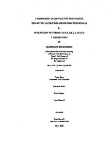
Figure 1: Blind source separation procedure performed in multistage ICA. Disadvantages: (F2) The separation performance is saturated before reaching a sufficient performance level because the independence assumption collapses in each narrow-band [7] (see, e.g., Sect. 5.3). (F3) Permutation among source signals and indeterminacy of each source gain in each frequency bin. Regarding the disadvantage (F3), various solutions have already been proposed [3, 8, 9, 10]. However, the collapse of the independence assumption, (F2), is a serious and inherent problem, and this prevents us from applying FDICA in a real acoustic environment with a long reverberation.
MSICA is conducted with the following steps. In the first stage, we perform FDICA to separate the source signals to some extent with the high-stability advantages (F1) of FDICA. In the second stage, we regard the separated signals of FDICA as the input signals for TDICA, and we remove the residual crosstalk components of FDICA by using TDICA. Finally, we regard the output signals of TDICA as the resultant separated signals. MSICA can achieve a high stability and a separation performance superior to that of conventional FDICA and TDICA. In the following sections, we describe details of the ICA-learning rules for each stage.
3.2. TDICA
In the first-stage ICA, we introduce the fast-convergence FDICA proposed by one of the authors [4]. We perform the signal separation procedure as described below (see FDICA in Fig. 1). In FDICA, first, the short-time analysis of observed signals x(t) is conducted by frame-by-frame discrete Fourier transform (DFT). By plotting the spectral values in a frequency bin of each microphone input frame by frame, we consider them as a time series. Hereafter, we designate the time series as X (f, t) =[X1 (f, t), · · · , XK (f, t)]T . Next, we perform signal separation using the complex-valued inverse of the mixing matrix, W (f) (f ), so that the L time-series (f) (f) output Z (f, t) = [Z1 (f, t), · · · , ZL (f, t)]T becomes mutually independent; this procedure can be given as
4.1. First-Stage ICA: FDICA
In the conventional BSS based on TDICA, each element of the separation filter matrix is represented as a FIR filter. We can optimize this separation filter system, by using the fullband observed signals themselves. TDICA has the following advantages and disadvantages. Advantages: (T1) We can treat the fullband speech signals where the independence assumption of sources usually holds. Disadvantages: (T2) The convergence degrades under reverberant conditions because the iterative rule for FIR filter learning is complicated. It is known that TDICA works only in the case of mixtures with a short-tap FIR filter, i.e., less than 100 taps. Also, TDICA fails to separate source signals under real acoustic environments because of the disadvantages (T2).
Z (f, t)
=
W (f) (f )X (f, t).
(2)
We perform this procedure with respect to all frequency bins. Finally, by applying the inverse DFT and the overlapadd technique to the separated time series Z (f, t), we reconstruct the resultant source signals in the time domain, z(t). In conventional FDICA , the optimal W (f) (f ) is obtained by the following iterative equation [3]:
4. PROPOSED METHOD: MSICA As described above, the conventional ICA methods have some disadvantages. However, note that the advantages and disadvantages of FDICA and TDICA are mutually complementary, i.e., (F2) can be resolved by (T1), and (T2) can be resolved by (F1). Hence, in order to resolve the disadvantages, we propose a new algorithm, MSICA, in which FDICA and TDICA are combined (see Fig. 1).
W (f) i+1 (f )
524
=
h
�
W (f) Φ(Z (f, t))Z H (f, t) i (f ) + α diag
� i (f) − Φ(Z (f, t))Z H (f, t) t W i (f ),
�� t
(3)
where h·it denotes the time-averaging operator, i is used to express the value of the i-th step in the iterations, and α is the step-size parameter. Also, we define the nonlinear vector function Φ(·) as Φ(Z (f, t)) ≡ [Φ(Z1 (f, t)), · · · , Φ(ZL (f, t))]T , Φ(Zl (f, t)) ≡
(R) tanh(Zl (f, t))+j
·
(I) tanh(Zl (f, t)),
where β is the step-size parameter. Since the Eq. (8) eval(b) uates only off-diagonal of hy (t)y (t)T it , we confirmed that the iterative equation of Eq. (8) could not achieve a superior separation performance under the reverberant condition (see Sect. 5.4). Namely, the source separation is not achieved by only using nonstationarity of signals. Therefore we use not only nonstationarity of signals but also time-delayed decorrelation approach. We expand Eq. (8) to the following equation to evaluate the off-diagonal of (b) hy (t)y (t − τ + d)T it for all time delays τ − d :
(4) (5)
where Re[Zl (f, t)] and Im[Zl (f, t)] are the real and imaginary parts of Zl (f, t), respectively.
[TDICA2]
4.2. Second-Stage ICA: TDICA
w(t2) i+1 (τ )
The output signals from TDICA (i.e., the separated signals of MSICA) can be given as
y(t) =
Q−1
X
w(t) (τ )z(t − τ ),
B Q−1
�(b) �−1 β X X n� diag y (t)y (t)T t B b=1 d=0
�(b) �
�(b) �−1 · diag y (t)y (t − τ + d)T t − diag y (t)y (t)T t
�(b) o (t2) · y (t)y (t − τ + d)T t wi (d), (9)
=
(6)
τ =0
w(t2) (τ ) + i
where y (t) = [y1 (t), · · · , yL (t)]T is the resultant separated (t) signal vector of MSICA, w(t) (τ ) = [wij (τ )]ij is the separation filter matrix, and Q is the length of the separation filter. The selection of TDICA is an important issue because the quality of resultant separated signals is determined by TDICA. In this study, we introduce three TDICA algorithms, i.e.,
Choi proposed the TDICA algorithm which optimizes the separation filter by minimizing the KLD between the joint probability density function and the marginal probability density function of the separated signals [12]. The KLD is given by
TDICA1: TDICA based on simultaneous decorrelation of nonstationary signals,
KLD
�
w(t) (τ )
Z
=
p(y (t)) log
TDICA2: TDICA based on combination of TDICA1 and time-delayed decorrelation approach, and
and compare these TDICA algorithms. First, we drive the TDICA1 algorithm. This optimizes the separation filter by minimizing the nonnegative cost function which takes the minimum value only when the second-order cross-correlation becomes zero if the source signals are nonstationary. The cost function is defined as follows (this cost function has been already proposed by Kawamoto et al. [11], however their derivation of learning rule includes mathematical error): �
w(t) (τ )
=
where p(·) is the joint probability density function, q(·) is the marginal probability density function, and T is the length of the separated signals. With a nonholonomic constraint, the iterative equation of the separation filter to minimize the KLD(w(t) (τ )) is given as (hereafter we designate the iterative equation as “TDICA3”):
w(t3) i+1 (τ )
w(t3) (τ ) i
=
� � diag h�(y (t))y (t − τ + d)T it d=0 o (t3) −h�(y (t))y (t − τ + d)T it wi (d). (11)
+α
t
�(y(t)) ≡
X
�
�(·) as
�T
tanh(y1 (t)), · · · , tanh(yL (t))
.
(12)
In this study, we compare the MSICA1, MSICA2, and MSICA3 in which FDICA followed by TDICA1, TDICA2, and TDICA2, respectively.
[TDICA1]
w
Q−1n
where we define the nonlinear vector function
(b)
where B is the number of local analysis blocks and h·it denotes the time-averaging operator for the b-th local analysis block. Equation (7) becomes zero only when yi (t) and yj (t) are uncorrelated for all of the local analysis blocks. � The correct iterative equation to minimize Q w(t) (τ ) is given by [6]
(t1) i+1 (τ )
q(yl (t))
[TDICA3]
�(b) �� � B � det diag y (t)y (t)T t 1 X log , (7)
�(b) 2B det y (t)y (t)T b=1
dy (t), (10)
l=1 t=0
TDICA3 [12]: TDICA based on minimization of KullbuckLeibler divergence (KLD),
Q
p(y (t)) −1 L TY Y
5. EXPERIMENTS AND RESULTS
B Q−1 � �−1 β X X n�
= w + y(t)y(t)T (b) t B b=1 d=0 �
�
�(b) �−1 (b) · y (t)y (t − τ + d)T t − diag y (t)y (t)T t
�(b) o (t1) · y (t)y (t − τ + d)T t wi (d), (8) (t1) (τ ) i
5.1. Experimental Setup A two-element array with the interelement spacing of 4 cm is assumed. We determined this interelement spacing by considering that the spacing should be smaller than half of
525
2.15 m
Noise Reduction Rate [dB]
3.12 m
1.56 m
5.73 m Loudspeakers 1.15 m
(Height : 1.35 m)
-30 40
Microphone array (Height : 1.35 m) (Spacing: 0.04m)
(Room height : 2.70 m)
10 8 6 4 2 0
32
64
128 256 512 1024 2048 4096 Number of Frequency Bins
Figure 3: Relation between separation performances and the number of frequency bins in conventional FDICA.
Figure 2: Layout of reverberant room used in experiments.
J
the minimum wavelength to avoid the spatial aliasing effect; it corresponds to 8.5/2 cm in 8 kHz sampling. The speech signals are assumed to arrive from two directions, −30◦ and 40◦ . The distance between the microphone array and the loudspeakers is 1.15 m (see Fig. 2). Two kinds of sentences, those spoken by two male and two female speakers selected from the ASJ continuous speech corpus for research, are used as the original speech samples. The sampling frequency is 8 kHz and the length of speech is limited to within 3 seconds. Using these sentences, we obtain 12 combinations with respect to speakers and source directions. In these experiments, we use the following signals as the source signals: the original speech convolved with the impulse responses specified by the reverberation time of 300 ms. This corresponds to 2400-taps FIR filter in 8 kHz. The impulse responses are recorded in a variable reverberation time room as shown in Fig. 2.
0.03 0.02 0.01 0
32
64
128 256 512 1024 2048 4096 Number of Frequency Bins
Figure 4: Relation between the number of frequency bins and the value of J defined by Eq. (16), which corresponds to the independence of subband signals.
5.3. Relation between Separation Performance and Number of Frequency Bins in FDICA
5.2. Objective Evaluation Score
In order to confirm the independence problem of narrowband signals in FDICA ((F2) described in Sect. 3.1), we carried out the preliminary experiment under the following analysis conditions. The number of frequency bins (frame length in DFT) is set to be from 32 to 4096, the frame shift is 16 taps, the window function is a Hamming window, the number of iterations in ICA is 30, and the step-size parameter α for iterations is set to be 1.0 × 10⁻⁵ . Figure 3 shows the NRR results for different numbers of frequency bins in FDICA. As shown in Fig. 3, the NRR of FDICA obviously degrades when the number of frequency bins becomes too large, and the separation performance is saturated before reaching a sufficient performance. This is because we transform the fullband signals into the narrowband signals and the independence assumption collapses in each frequency bin, particularly when the number of frequency bins is large. In order to confirm the fact, we newly define the following objective measure to quantify an independence, and investigate the relation between the number of frequency bins and the independence among subband signals. D �
��
H J =
diag Φ(Z (f, t))Z (f, t) t E
�
(16) − Φ(Z (f, t))Z H (f, t) t ,
Noise reduction rate (NRR), defined as the output signalto-noise ratio (SNR) in dB minus input SNR in dB, is used as the objective evaluation score in this experiment. The SNRs are calculated under the assumption that the speech signal of the undesired speaker is regarded as noise. The NRR is defined as 2 � 1 X� (O) (I) SNRl − SNRl , (13) NRR ≡ 2 l=1 P 2 f |Hll (f )Sl (f )| (O) SNRl , (14) = 10 log10 P 2 f |Hln (f )Sn (f )| P 2 f |All (f )Sl (f )| (I) = 10 log10 P , (15) SNRl 2 f |Aln (f )Sn (f )| (O)
0.08 0.07 0.06 0.05 0.04
(I)
and SNRl are the output SNR and the where SNRl input SNR, respectively, and l 6= n. Also, Sl (f ) is the frequency-domain representation of the source signal, sl (t), Hij (f ) is the element in the i th row and the j th column of the matrix H (f ) = W (MSICA) (f )A(f ) where W (MSICA) (f ) denotes the entire separation process in MSICA including both FDICA and TDICA and A(f ) is the mixing matrix which corresponds to the frequency-domain representation of the room impulse responses described in Sect. 2.
f
526
Noise Reduction Rate
High-Independence
� �
Robust against Reverberation
z : 19 8x ~/ yu5 0,7 6 v ~ -t + }5 4 z|13{ 2 x y0/
LowIndependence
Poor against Reverberation
x/ vu-,w . su*,t +
� � ���
Number of Frequency Bins
CEDGF@HJILK
CMDNF@HJIPO
CEDGF@HJIPQ
� � � � � � � �
Small
;�=@?BA
�
� �
� �
� ��]N��_a`c ����b%��de��_f[g �� �`h ��[c �ik �!j� #"l�%m� $�bB �%&' Z� �[� �\^ no$� m#(�pr) q �
���
� �
RGS�TVUXW�YVT
Figure 6: Comparison of separation performance between MSICA1, MSICA2, and MSICA3.
Large
Figure 5: Trade-off relation among the independence of subband signals and robustness against reverberation. TDICA1 and TDICA2, we divided the signals equally into B parts (B = 1–10). We chose the optimal B and number of iterations for each combination of speaker because the convergence is different for every combination. As for the FDICA part in MSICA, the analysis conditions are the same as those given in Sect. 5.3, except for the number of frequency bins (which is fixed at 1024 bins). Figure 6 shows the NRR results in the MSICA1, MSICA2 and MSICA3. Figure 6 shows that TDICA1 can not achieve a signal separation under the reverberant condition. Comparing MSICA1 with MSICA2 in Fig. 6, we confirm that TDICA2 can achieve a superior separation performance to TDICA1. These results show that it is necessary to evaluate correlations of different times to achieve a superior performance. TDICA3 can also achieve a superior separation performance to TDICA1. The separation performances of MSICA2 and MSICA3 are superior to that of FDICA and the improvements of the separation performance from FDICA are not so different. Thus, the use of FDICA with TDICA2 or TDICA3 is effective in the proposed MSICA structure.
where k · k is frobenius norm of matrix. This measure J is a part of the iterative equation (3) and has no dimension. Therefore the absolute value of J is meaningless itself, however, the relative value between the different numbers of frequency bins is important. If narrow-band signals become mutually independent, the measure J becomes zero. Also we can consider that the independence of subband signals is high when J is small. In order to evaluate the independence of real narrow-band speech signals, we carried out the experiment in which the input signal, Y (f, t), in Eq. (16) is regarded as the perfectly separated sources, i.e., original speech samples. Figure 4 shows the relation between the number of frequency bins and the value of J which corresponds to the independence of subband signals. Figure 4 shows that the independence decreases as the number of frequency bins increases, especially when the number of frequency bins is large. Above-mentioned experimental results clarify the disadvantage that the separation performance is saturated in FDICA because we transform the fullband signals into the narrow-band signals. We should lengthen the separation filter (or FFT length for analysis) when we confront with a long reverberation. In this case, however, the independence of subband signals decreases. Thus, there is a trade-off relation among the independence of subband signals and robustness against reverberation as shown in Figure 5. On the basis of these results, we should cascade another signal processing analysis, e.g., TDICA, with FDICA to obtain the further separation performances.
5.5. Comparison between MSICA2 and MSICA3
In order to compare MSICA2 and MSICA3 in detail, we evaluate the separation performances of MSICA3 and MSICA2 with the various number of local blocks B. In TDICA2 part in MSICA2, the utilization of large B is effective because it can evaluate the nonstationarity of the signals. Figure 7 shows the NRR results in the MSICA3 and MSICA2 with the various B. The separation performance is improved as the B is increased, however, the larger B is not the best for improving the separation performance. In addition, the 5.4. Comparison of Separation Performance between separation performances of MSICA3 and MSICA2 with the MSICAs optimal B are not so different. Therefore, MSICA3 is more We carried out the experiments using MSICA1, MSICA2, feasible than MSICA2 because MSICA3 does not require and MSICA3 to evaluate the contribution of TDICA1, TDICA2, the estimation of the optimal B. and TDICA3 for improving the separation performances under reverberant conditions. The analysis conditions of 5.6. Discussion on Combination Order in MSICA these experiments are as follows: the filter length Q is As described in the previous section, the combination of set to be 2048taps, the maximum number of iterations is FDICA and TDICA can contribute to the improvement 500, and the step-size parameter β for iterations is set to of separation. In this combination, the advantage (F1) of be 5.0 × 10⁻⁴ for TDICA1, 1.0 × 10⁻³ for TDICA2, and FDICA is useful in the initial step of separation procedure 1.0 × 10⁻⁶ for TDICA3. As for the local analysis block for
527
��� O NP
and the advantage (T1) of TDICA is also useful in the later step. Therefore we use FDICA as the first-stage ICA and TDICA as the second-stage ICA. In order to confirm the availability of this combination order, we compare the proposed combination with the combination in which TDICA is used in the first stage and FDICA is used in the second stage ( hereafter we designate this swapped combination as ”MSICA4”).
M
N4 �
G DFE B C B
S� O�
@?A ?= >
The experiment of MSICA4 was carried out in the following manner. As for TDICA part in MSICA4, TDICA2 is used, the number of local analysis blocks, B, is fixed at 3, and the filter length is 8 taps improved best the separation performance in TDICA2. This TDICA2 can obtain the NRR of 6.0 dB. As for FDICA part in MSICA4, the analysis conditions are the same as those given in Sect. 5.3, except for the number of frequency bins (which is fixed at 1024 bins). As the result, the NRR of 7.5 dB is obtained in MSICA4, and this performance is better than that of simple TDICA but is poorer than those of MSICA2, MSICA3, and simple FDICA. In MSICA4, the separation performance is still improved by using FDICA in the second stage, however, the separation performance is saturated because of the disadvantage (F2) of FDICA. MSICA4 can not achieve the separation performance of 9.4 dB which corresponds to NRR of simple FDICA. This reason is that FDICA in this paper uses the beamforming technique and the directivity pattern of the array which provide a good initial value of the separation matrix to improve the convergence [4], however, such kind of information is no longer valid in the combination order of MSICA4 because we can not know the effective positions of the array elements after the first-stage TDICA and can not depict the directivity pattern. Thus the separation performance of MSICA4 is almost equal to that of a raw FDICA without the beamforming technique (from [4] we can see the NRR of about 7.5 dB at the 30-iteration point). This fact indicates that the swapped combination order of MSICA4 has no contribution to the improvement of the separation performance, and the proposed combination order of MSICA2 and MSICA3 (FDICA in the first stage and TDICA in the second stage) is essential.
Q
�< N�