Scenario-based Stochastic Constraint Programming
arXiv:0905.3763v1 [cs.AI] 22 May 2009
Suresh Manandhar and Armagan Tarim Department of Computer Science University of York, England email: {suresh,at}@cs.york.ac.uk
Abstract To model combinatorial decision problems involving uncertainty and probability, we extend the stochastic constraint programming framework proposed in [Walsh, 2002] along a number of important dimensions (e.g. to multiple chance constraints and to a range of new objectives). We also provide a new (but equivalent) semantics based on scenarios. Using this semantics, we can compile stochastic constraint programs down into conventional (nonstochastic) constraint programs. This allows us to exploit the full power of existing constraint solvers. We have implemented this framework for decision making under uncertainty in stochastic OPL, a language which is based on the OPL constraint modelling language [Hentenryck et al., 1999]. To illustrate the potential of this framework, we model a wide range of problems in areas as diverse as finance, agriculture and production.
1 Introduction Many decision problems contain uncertainty. Data about events in the past may not be known exactly due to errors in measuring or difficulties in sampling, whilst data about events in the future may simply not be known with certainty. For example, when scheduling power stations, we need to cope with uncertainty in future energy demands. As a second example, nurse rostering in an accident and emergency department requires us to anticipate variability in workload. As a final example, when constructing a balanced bond portfolio, we must deal with uncertainty in the future price of bonds. To deal with such situations, [Walsh, 2002] has proposed an extension of constraint programming, called stochastic constraint programming, in which we distinguish between decision variables, which we are free to set, and stochastic (or observed) variables, which follow some probability distribution. This framework combines together some of the best features of traditional constraint satisfaction, stochastic integer programming, and stochastic satisfiability. In this paper, we extend the expressivity of this framework considerably by adding multiple chance constraints, as well as a range of objective functions like maximizing the downside. We show how such stochastic constraint programs can
Toby Walsh Cork Constraint Computation Centre University College Cork, Ireland. email:
[email protected].
be compiled down into conventional (non-stochastic) constraint programs using a scenario-based interpretation. This compilation allows us to use existing constraint solvers without any modification, as well as call upon the power of hybrid solvers which combine constraint solving and integer programming techniques. We also propose a number of techniques to reduce the number of scenarios and to generate robust solutions. We have implemented this framework for decision making under uncertainty in a language called stochastic OPL. This is an extension of the OPL constraint modelling language [Hentenryck et al., 1999]. Finally, we describe a wide range of problems that we have modelled in stochastic OPL that illustrate some of its potential.
2 Stochastic constraint programs In a one stage stochastic constraint satisfaction problem (stochastic CSP), the decision variables are set before the stochastic variables. The stochastic variables, independent of the decision variables, take values with probabilities given by a probability distribution. This models situations where we act now and observe later. For example, we have to decide now which nurses to have on duty and will only later discover the actual workload. We can easily invert the instantiation order if the application demands, with the stochastic variables set before the decision variables. Constraints are defined (as in traditional constraint satisfaction) by relations of allowed tuples of values. Constraints can, however, be implemented with specialized and efficient algorithms for consistency checking. We allow for both hard constraints which are always satisfied and “chance constraints” which may only be satisfied in some of the possible worlds. Each chance constraint has a threshold, θ and the constraint must be satisfied in at least a fraction θ of the worlds. A one stage stochastic CSP is satisfiable iff there exists values for the decision variables so that, given random values for the stochastic variables, the hard constraints are always satisfied and the chance constraints are satisfied in at least the given fraction of worlds. Note that [Walsh, 2002] only allowed for one (global) chance constraint so the definition here of stochastic constraint programming is strictly more general. In a two stage stochastic CSP, there are two sets of decision variables, Vd1 and Vd2 , and two sets of stochastic variables, Vs1 and Vs2 . The aim is to find values for the variables in Vd1 ,
so that given random values for Vs1 , we can find values for Vd2 , so that given random values for Vs2 , the hard constraints are always satisfied and the chance constraints are again satisfied in at least the given fraction of worlds. Note that the values chosen for the second set of decision variables Vd2 are conditioned on both the values chosen for the first set of decision variables Vd1 and on the random values given to the first set of stochastic variables Vs1 . This can model situations in which items are produced and can be consumed or put in stock for later consumption. Future production then depends both on previous production (earlier decision variables) and on previous demand (earlier stochastic variables). An m stage stochastic CSP is defined in an analogous way to one and two stage stochastic CSPs. Note that [Walsh, 2002] insisted that the stochastic variables take values independently of each other. This prevents us representing a number of common situations. For example, if the market goes down in the first quarter, it is probably more likely to go down in the second quarter. A second stage stochastic variable representing the market index is therefore dependent on the first stage stochastic variable representing the market index. There is, however, nothing in the semantics given for stochastic constraint programs nor in the solution methods proposed in [Walsh, 2002] that used this assumption. We therefore allow later stage stochastic variables to take values which are conditioned by the earlier stage stochastic variables. A stochastic constraint optimization problem (stochastic COP) is a stochastic CSP plus a cost function defined over the decision and stochastic variables. In [Walsh, 2002], the only goal considered was to find a solution that satisfies the stochastic CSP which minimizes or maximizes the expected value of the objective function. We now extend this to a much wider range of goals. For example, we might wish to limit the downside (i.e. maximize the least value of the cost function), or to minimize the spread (i.e. minimize the difference between the least and the largest value of the cost function).
3 Scenario-based semantics In [Walsh, 2002], a semantics for stochastic constraint programs is given based on policies. A policy is a tree of decisions. Each path in a policy represents a different possible scenario (set of values for the stochastic variables), and the values assigned to decision variables in this scenario. To find satisfying policies, [Walsh, 2002] presents backtracking and forward checking algorithms which explores the implicit AND/OR graph. Stochastic variables give AND nodes as we must find a policy that satisfies all their values, whilst decision variables give OR nodes as we only need find one satisfying value. An alternative semantics, which suggests an alternative solution method, comes from a scenario-based view [Birge and Louveaux, 1997]. A scenario is any possible set of values for the stochastic variables. Thus, a scenario is associated with each path in the policy. Within each scenario, we have a conventional (non-stochastic) constraint program to solve. We simply replace the stochastic variables by the values taken in the scenario, and ensure that the values
found for the decision variables are consistent across scenarios. Note that certain decision variables are shared across scenarios. The first stage decisions are, for example, shared by all scenarios. The great advantage of this approach is that we can use conventional constraint solvers to solve stochastic constraint programs. We do not need to implement specialized solvers. Of course, there is a price to pay as the number of scenarios grows exponentially with the number of stages. However, our results show that a scenario-based approach is feasible for many problems. Indeed, we observe much better performance using this approach on the production planning example introduced in [Walsh, 2002]. In addition, as we discuss later, we have developed a number of techniques like Latin hypercube sampling to reduce the number of scenarios considered.
4 Stochastic OPL We have implemented this framework on top of the OPL constraint modelling language [Hentenryck et al., 1999]. An OPL model consists of two parts: a set of declarations, followed by an instruction. Declarations define the data types, (input) data and the (decision) variables. An OPL instruction is either to satisfy a set of constraints or to maximize/minimize an objective function subject to a set of constraints. We have extended the declarations to include the declaration of stochastic variables, and the instructions to include chance constraints, and a range of new goals like maximizing the expectation of an objective function.
4.1
Variable declaration
We now declare both decision and stochastic variables. Stochastic variables are set according to a probability distribution using a command of the form: stoch ; Where is (as with decision variables) a data type (e.g. a range of values, or an enumerated list of values), is (as with decision variables) the variable name, and defines the probability distribution of the stochastic variable(s). Probability distributions include uniform, poisson(lambda), and user defined via a list of (not necessarily normalized) values. Other types of distribution can be supported as needed. We insist that stochastic variables are arrays, with the last index describing the stage. Here are some examples: stoch 0..1 market[Years] uniform; stoch 100..102 demand[Quarter] {1,2,3}; In the first, we have a 0/1 variable in each year which takes either value with equal probability. In the last, we have a demand variable for each quarter, which takes the value 100 in 1 out of 6 cases, 101 in 2 out 6 cases, and 102 in the remaining 3 cases.
4.2
Constraint posting
We can post both hard constraints (as in OPL) and chance constraints. Chance constraints hold in some but not necessarily all scenarios. They are posted using a command of the form:
prob() ; Where is any OPL constraint, is any of the arithmetically comparison operations (=,,, =) and is any arithmetic expression (it may contain decision variables or may just be a rational or a float in the range 0 to 1). For example, the following command specifies the chance constraint that in each quarter the demand (a stochastic variable) does not exceed the production (a decision variable) plus the stock carried forward in each quarter (this auxiliary is modelled, as in conventional constraint programming, by a decision variable) with 80% probability: forall(i in 1..n) prob(demand[i] = 0.80; Constraints which are not chance constraints are hard and have to hold in all possible scenarios. For example, the stock carried forwards is computed via the hard constraint: forall(i in 1..n) stock[i+1] = stock[i] + production[i] - demand[i];
4.3
Optimization
Stochastic OPL supports both stochastic constraint satisfaction and optimization problems. We can maximize or minimize the expectation of an objective function. For example, in the book production example of [Walsh, 2002], we can minimize the expected cost of storing surplus books. Each book costs $1 per quarter to store. This can be specified by the following (partial) model: minimize expected(cost) subject to cost = sum(i in 1..n) max(stock[i+1],0); forall(i in 1..n) stock[i+1] = stock[i] + production[i] - demand[i]; Stochastic OPL also supports a number of other optimization goals. For example: minimize spread(profit) maximize downside(profit) minimize upside(cost) The spread is the difference between the value of the objective function in the best and worst scenarios, whilst the downside (upside) is the minimum (maximum) objective function value a possible scenario may take.
5 Compilation of stochastic OPL These stochastic extensions are compiled down into conventional (non-stochastic) OPL models automatically by exploiting the scenario-based semantics. The compiler is written in Lex and Yacc, with a graphical interface in Visual C++. Compilation involves replacing stochastic variables by their possible values, and decision variables by a ragged array of decision variables, one for each possible scenario. Consider again the chance constraint:
prob( demand[i] = 0.80; This is compiled into a sum constraint of the form: sum(j in Scenarios) p[j]* (demand[i,j] = 0.80; Where Scenarios is the set of scenarios, p[j] is the probability of scenario j, demand[i,j] is the demand in scenario j and quarter i, etc. Note that the bracketing of the inequality reifies the constraint so that it takes the value 1 if satisfied and 0 otherwise. Hard constraints are also transformed. Consider, for example, the hard constraint: wealth[t] = bonds[t] + stocks[t]; This is compiled into a forall constraint of the form: forall(j in Scenarios) wealth[t,j] = bonds[t,j] + stocks[t,j]; Where wealth[t,j] is the wealth at time t in scenario j, etc. Maximization and minimization instructions are also transformed. Consider, for example, the optimization instruction: maximize expected(wealth[n]) subject to ... This is compiled into an instruction of the form: maximize sum(j in Scenarios) p[j]*wealth[n,t] subject to ... The rest of the stochastic OPL model is transformed in a similar manner.
6 Value of information and stochastic solutions For stochastic optimization problems, we compute two statistics which quantify the importance of randomness. The value of a stochastic solution (VSS) is the difference in the objective function for the stochastic problem (call it the stochastic solution, SS) and the objective value for the deterministic problem computed by replacing stochastic variables by their expectations (call it the expected value solution, EVS): V SS = SS − EV S. This computes the benefit of knowing the distributions of the stochastic variables. Clearly, VSS is non-negative. We also compute the expected value of the wait-and-see solution (WSS). To calculate this, we give the stochastic variables values according to their probability distributions, and then find the best values for the decision variables. The difference between WSS and SS is the expected value of perfect information (EVPI): EV P I = W SS − SS. This measures how much more you can expect to win if you have perfect information about the stochastic components of the problem. In other words, EVPI measures the value of knowing the future with certainty. This is therefore the most that should be spent in gathering information about the uncertain world.
7 Scenario reduction
8.1
One problem with a scenario-based approach is the large number of scenarios, each of which introduces new decision variables. We have therefore implemented several techniques to reduce the number of scenarios. The simplest is to consider just a single scenario in which stochastic variables take their expected values. This is supported with the command:
This problem comes from [Walsh, 2002]. The results in Table 1 show that a scenario-based approach offers much better performance on this problem than the forward checking or backtracking tree search algorithms also introduced in this paper. The problem involves planning production over m quarters. In each quarter, we expect to sell between 100 and 105 copies of a book. To keep customers happy, we want to satisfy demand over all m quarters with 80% probability. This problem is modelled by an m stage stochastic CSP. There are m decision variables, xi representing production in each quarter. There are also m stochastic variables, yi representing demand in each quarter. To limit stock carried forward, we use a simple heuristic which picks the smallest possible values for the decision variables. An alternative is to convert the problem into an optimization problem with a cost to keep books in store. We do not explore this option here, though it is very easy to implement in stochastic OPL, as we cannot then compare our results with those of the forward checking or backtracking algorithms from [Walsh, 2002].
scenario expected; The user may also be content to consider just the most probable scenarios and ignore rare events. We support this with the command: scenario top ; Another option is to use Monte Carlo sampling. The user can specify the number of scenarios to sample using a command of the form: scenario sample ; The probability distributions of the stochastic variables is used to bias the construction of these scenarios. We also implemented one of the best sampling methods from experimental design, and one of the best scenario reduction methods from operations research. Latin hypercube sampling [McKay et al., 1979], ensures that a range of values for a variable are sampled. Suppose we want n sample scenarios. We divide the unit interval into n intervals, and sample a value for each stochastic variable whose cumulative probability occurs in each of these interval. We then construct n sample scenarios from these values, enforcing the condition that the samples use each value for each stochastic variable exactly once. More precisely, let fi (a) be the cumulative probability that Xi takes the value a or less, πi (j) be the jth element of a random permutation πi of the integers {0, . . . , n − 1}, and r be a random number uniformly drawn from [0, 1]. Then, the jth Latin hypercube sample value for the stochastic variable Xi is: fi−1 (
πi (j) + r ) n
Finally, we implemented a scenario reduction method used in stochastic programming due to Dupacova, Growe-Kuska and Romisch [Dupacova et al., 2002]. They report power production planning problems on which this method offers 90% accuracy sampling 50% of the scenarios and 50% accuracy sampling just 2% of the scenarios. The method heuristically deletes scenarios to approximate as closely as possible the original scenarios according to a Fortet-Mourier metric on the stochastic parameter space.
8 Some examples To illustrate the potential of this framework for decision making under uncertainty, we now describe a wide range of problems that we have modelled. In the first problem, we compare a scenario-based approach to the previous tree search methods for solving stochastic constraint satisfaction problems. In the next three problems, we illustrate the effectiveness of the different scenario reduction techniques.
8.2
Production planning
Portfolio management
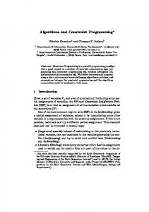
This portfolio management problem of [Birge and Louveaux, 1997] can be modelled as a stochastic COP. Suppose we have $P to invest in any of I investments and we wish to exceed a wealth of $G after t investment periods. To calculate the utility, we suppose that exceeding $G is equivalent to an income of q% of the excess while not meeting the goal is equivalent to borrowing at a cost r% of the amount short. This defines a concave utility function for r > q. The uncertainty in this problem is the rate of return, which is a random variable, on each investment in each period. The objective is to determine the optimal investment strategy, which maximizes the investor’s expected utility. The problem has 8 stages and 5760 scenarios. To compare the effectiveness of the different scenario reduction algorithms, we adopt a two step procedure. In the first step, the scenario reduced problem is solved and the first period’s decision is observed. We then solve the full-size (non scenario reduced) problem to optimality with this first decision fixed. The difference between the objective values of these two solutions is normalized by the range [optimal solution, observed worst solution] to give a normalized error for committing to the scenario reduced first decision. In Fig. 1, we see that Dupacova et al’s algorithm is very effective, that Latin hypercube sampling is a small distance behind, and both are far ahead of the most likely scenario method (which requires approximately half the scenarios before the first decision is made correctly).
8.3
Yield management
Farmers must deal with uncertainty since weather and many other factors affect crop yields. In this example (also taken from [Birge and Louveaux, 1997]), we must decide on how many acres of his fields to devote to various crops before the planting season. A certain amount of each crop is required for cattle feed, which can be purchased from a wholesaler if not raised on the farm. Any crop in excess of cattle feed can be sold up to the EU quota; any amount in excess of this quota
No. Stages 1 2 3 4 5 6
Backtracking (BT) Nodes CPU/sec 28 0.01 650 0.09 17,190 2.72 510,356 83.81 15,994,856 3,245.99 – –
Forward Checking (FC) Nodes CPU/sec 10 0.01 148 0.03 3,604 0.76 95,570 19.07 2,616,858 509.95 – –
Failure 4 4 8 42 218 1260
Scenario-Based (SB) Choice Points CPU/sec 5 0.00 8 0.02 24 0.16 125 1.53 690 18.52 4035 474.47
Table 1: A Comparison of BT, FC and SB Approaches on the Book Production Problem (Sec.8.1) Error (%) Error (%) c× × × × × × × × × × × × × × × × × × × × × × × × × × × 100 × 100 × r r Dupacova Alg. Dupacova Alg. 90 90 × c c Latin Hypercube Latin Hypercube 80 80 × Mostlikely Scen. × Mostlikely Scen. 70 70 × × 60 60 × × 50 50 × × 40 40 c × × × 30 30 × c × 20 20 ×× rc c cc × × × × c 10 c c c crcrrcrr r c c c × 10 ×c × × × × ×c × c × c r crcrrrcrcrcrrrcrrcrcrrcr ccrcrcrcrrcrcrcrcrrrccrrcrcrcrcrcrrcrccrcrcrrr× crcr ×cr ×cr ×rc ×rc ×cr ×cr ×cr ×cr ×cr ×cr r r r r r r r r r ×cr ×cr ×cr ×cr ×cr ×cr ×cr ×cr ×cr ×cr ×cr ×cr c c c c c c × × 0 0 0 10 20 30 40 50 60 70 80 90 100 0 10 20 30 40 50 60 70 80 90 100 Number of Scenarios (%) Number of Scenarios (%) Figure 1: Portfolio Management Error (%) 100 × r × Dupacova Alg. 90 c Latin Hypercube 80 × Mostlikely Scen. 70 60 50 40 30 ××××× 20 10 0 cr cr cr cr cr cr cr ×cr ×cr ×cr ×cr ×cr ×cr ×cr ×cr ×cr ×cr ×cr ×cr ×cr ×cr 0 10 20 30 40 50 60 70 80 90 100 Number of Scenarios (%) Figure 2: Agricultural Yield Management will be sold at a low price. Crop yields are uncertain, depending upon weather conditions during the growing season. This problem has 4 stages and 10,000 scenarios. In Fig. 2, we again see that Dupacova et al’s algorithm and Latin hypercube sampling are very effective, and both are far ahead of the most likely scenario method (which requires approximately one third the scenarios before the first decision is made correctly).
8.4
Production/Inventory control
Uncertainty plays a major role in production and inventory planning. In this simplified production/inventory planning example, there is a single product, a single stocking point,
Figure 3: Production/Inventory Control production capacity constraints and stochastic demand. The objective is to find the minimum expected cost policy. The cost components take into account holding costs, backlogging costs, fixed replenishment (or setup) costs and unit production costs. The optimal policy gives the timing of the replenishments as well as the order-up-to-levels. Hence, the exact order quantity can be known only after the realization of the demand, using the scenario dependent order-up-to-level decisions. This problem has 5 stages and 1,024 scenarios. In Fig. 3, we again see that Dupacova et al’s algorithm and Latin hypercube sampling are very effective, but both are now only a small distance ahead of the most likely scenario method.
9 Robust solutions Inspired by robust optimization methods in operations research [Kouvelis and Yu, 1996], stochastic OPL also allows us to find robust solutions to stochastic constraint programs. That is, solutions in which similar decisions are made in the different scenarios. It will often be impossible or undesirable for all decision variables to be robust. We therefore identify those decision variables whose values we wish to be identical across scenarios using commands of the form: robust ; For example, in production/inventory problem of Sec.8.4 the decision variables “order-up-to-levels” and “replenishment periods” can be declared as robust variables. The values of these two sets of decision variables are then fixed at the beginning of the planning horizon. A robust solution dampens the nervousness of the solution, an area of very active re-
search in production/inventory management. As the expected cost of the robust solution is always higher, the tradeoff between nervousness and cost may have to be taken into account.
10 Related and future work Stochastic constraint programs are closely related to Markov decision problems (MDPs) [Puterman, 1994]. Stochastic constraint programs can, however, model problems which lack the Markov property that the next state and reward depend only on the previous state and action taken. The current decision in a stochastic constraint program will often depend on all earlier decisions. To model this as an MDP, we would need an exponential number of states. Another significant difference is that stochastic constraint programs by using a scenario-based interpretation can immediately call upon complex and powerful constraint propagation techniques. Stochastic constraint programming was inspired by both stochastic integer programming and stochastic satisfiability [Littman et al., 2000]. It is designed to take advantage of some of the best features of each framework. For example, we are able to write expressive models using non-linear and global constraints, and to exploit efficient constraint propagation algorithms. In operations research, scenarios are used in stochastic programming. Indeed, the scenario reduction techniques of Dupacova, Growe-Kuska and Romisch [Dupacova et al., 2002] implemented here are borrowed directly from stochastic programming. There are a number of extensions of conventional constraint satisfaction problem to model constraints that are uncertain, probabilistic or not necessarily satisfied. For example, in probabilistic constraint satisfaction each constraint has a certain probability independent of all other probabilities of being part of the problem [Fargier and Lang, 1993] whilst in semi-ring constraint satisfaction each tuple in a constraint has a value associated with it [Bistarelli et al., 1996]. However, none of these extensions deal with variables that may have uncertain or probabilistic values. Stochastic constraint programming could, however, easily be combined with most of these techniques.
11 Conclusions To model combinatorial decision problems involving uncertainty and probability, we have extended the stochastic constraint programming framework proposed in [Walsh, 2002] along a number of important dimensions. In particular, we have relaxed the assumption that stochastic variables are independent, and added multiple chance constraints as well as a range of objective functions like maximizing the downside. We have also provided a new (but equivalent) semantics for stochastic constraint programs based on scenarios. Based on this semantics, we can compile stochastic constraint programs down into conventional (non-stochastic) constraint programs. The advantage of this compilation is that we can use the full power of existing constraint solvers without any modification. We have also proposed a number of techniques to reduce the number of scenarios, and to generate robust solutions.
We have implemented this framework for decision making under uncertainty in a language called stochastic OPL. This is an extension of the OPL constraint modelling language [Hentenryck et al., 1999]. To illustrate the potential of this framework, we have modelled a wide range of problems in areas as diverse as finance, agriculture and production. There are many directions for future work. For example, we want to allow the user to define a limited set of scenarios that are representative of the whole. As a second example, we want to explore more sophisticated notions of solution robustness (e.g. limiting the range of values used by a decision variable).
Acknowledgements This project was funded by EPSRC under GR/R30792, and the Science Foundation Ireland. We thank the members of the APES Research Group and 4C Lab for their feedback.
References [Birge and Louveaux, 1997] J. R. Birge and F. Louveaux. Introduction to Stochastic Programming. Springer-Verlag, New York, 1997. [Bistarelli et al., 1996] S. Bistarelli, H. Fargier, U. Montanari, F. Rossi, T. Schiex, and G. Verfaillie. Semi-ring based CSPs and valued CSPs: Basic properties and comparison. In M. Jample, E. Freuder, and M. Maher, editors, Over-Constrained Systems, pages 111–150. SpringerVerlag, 1996. LNCS 1106. [Dupacova et al., 2002] J. Dupacova, N. Growe-Kuska, and W. Romisch. Scenario reduction in stochastic programming: an approach using probability metrics. Mathematical Programming, To appear, 2002. [Fargier and Lang, 1993] H. Fargier and J. Lang. Uncertainty in constraint satisfaction problems: a probabilistic approac h. In Proceedings of ECSQARU. Springer-Verlag, 1993. LNCS 747. [Hentenryck et al., 1999] P. Van Hentenryck, L. Michel, L. Perron, and J-C. Regin. Constraint programming in OPL. In G. Nadathur, editor, Principles and Practice of Declarative Programming, pages 97–116. SpringerVerlag, 1999. Lecture Notes in Computer Science 1702. [Kouvelis and Yu, 1996] P. Kouvelis and G. Yu. Robust Discrete Optimization and Its Applications. Nonconvex optimization and its applications: volume 14. Kluwer, 1996. [Littman et al., 2000] M.L. Littman, S.M. Majercik, and T. Pitassi. Stochastic Boolean satisfiability. Journal of Automated Reasoning, 2000. [McKay et al., 1979] M.D. McKay, R.J. Beckman, and W.J. Conover. A comparison of three methods for selecting values of input variables in the analysis of output from a computer code. Technometrics, 21(2):239–245, 1979. [Puterman, 1994] M.L. Puterman. Markov decision processes: discrete stochastic dynamic programming. John Wiley and Sons, 1994. [Walsh, 2002] Toby Walsh. Stochastic constraint programming. In Proceedings of the 15th ECAI. European Conference on Artificial Intelligence, IOS Press, 2002.