Multivariable Control Enhancement of an Earthmoving Vehicle Working Cycle 1
Rong Zhang , Andrew G. Alleyne, Don E. Carter Department of Mechanical and Industrial Engineering University of Illinois at Urbana-Champaign 1206 W Green Street, Urbana, IL 61801 Tel: (217)244-0845, Fax: (217)244-6534 Emails:
[email protected],
[email protected],
[email protected]
Abstract A general operation of an earthmoving vehicle involves the coordination of a multivariable powertrain and the execution of a specific task in a repetitive fashion. Currently, this operation still depends heavily on human expertise. This dependence is an impediment to increased productivity. The purpose of this research is to automate the coordination of a multi-input multi-output (MIMO) nonlinear electro-hydraulic powertrain and to validate the performance and efficiency improvements in a typical working cycle.
A robust gain scheduling method is
developed to design a global controller and to analyze its robust stability and robust performance. To experimentally validate these analytical properties, the global controller is tested on an Earthmoving Vehicle Powertrain Simulator (EVPS), a Hardware -In-the-Loop (HIL) environment for control prototyping. The experiments include the humanoperated reference tracking and the human-operated working cycle. Performances of the same powertrain with and without the controller are compared. The results show the significant control benefits in the performance, the ease of operation, and the energy and time efficiency.
1 Introduction Earthmoving is an industry that requires tremendous resources, which includes expensive equipment, experienced operators, considerable energy consumption and intelligent operation planning. In recent years, the competition in this industry has pushed a movement toward higher level of automation to improve productivity, performance, and safety [1]. This automation trend is seen at the component level, the machine system level, the path planning level, the fleet operation level, and the project management level. The control problems at different levels have attracted many research efforts. Non-exhaustive examples at the component level include the performance analysis and improvement of valves [2-6], pumps [7-12], and actuators [13]. At path planning and operation level, some simulation and experimental works are reported by [14-19]. Compared to these explorations at the higher and lower levels, the research at the machine level has been relatively 1 Currently with the Electrical and Controls Integration Lab at General Motors R&D and Planning, 30500 Mound Road, MC 480-106-390, Warren, MI 48090, Tel: (586) 986-8740, Fax: (586) 986-3003.
1
limited. Successful machine level control is the necessary step toward fully automated off-highway engineering and has the most potential to be immediately implemented under the existent infrastructure. Currently, there appears to be a gap between the lower and the higher levels of research in earthmoving automation. The goal of this research is to solve the general automation problem at the machine powertrain level, and to validate this solution using a Hardware-In -the-Loop (HIL) technique.
Control Control Imp lem ent
2 Hydr. Hydr. Pump Pump
5 4
1 Engine Engine
3 Steering
Drive Drive
Figure 1 Proposed earthmoving vehicle powertrain with MIMO control
Figure 2 Earthmoving Vehicle Powertrain Simulator
The challenges of the control problem are the inter-load coupling and the nonlinearities.
A general
earthmoving vehicle powertrain in Fig. 1 is modeled as a multi-input multi-output (MIMO) nonlinear system. At a specific operating point, it is linearized to a LTI system and a local controller is designed using an H∞ algorithm. A gain scheduling method is used to schedule the local controllers at different operating points such that the large working range is covered. A small gain condition is used to guarantee the robust stability and robust performance of the global controller[Zhang, 2003 #182].
2
Implement Ref. Powertrain Controller
Steering Ref. Drive Ref.
MOTOR
PC2
)(
)(
)(
(PC3)
(PC3)
PC1 PC3 Pump
Engine
Drive
Steering
Implement
Figure 3 Schematic of the Earthmoving Vehicle Powertrain Simulator The challenges of the performance evaluation are the infeasibility of field tests and the complexity of human-operated working cycle. To find a general solution for a class of earthmoving vehicle powertrains, it is not desirable to limit the experiments to one specific product model. For budget and safety reasons, it is neither feasible to use a whole fleet of equipment. Under these considerations, a flexible HIL testbed, namely the Earthmoving Vehicle Powertrain Simulator in Fig. 2 was developed at the University of Illinois at Urbana-Champaign. Using the engine emulator in a computer PC1 and the load emulators in another computer PC3, it is capable of physically representing different earthmoving vehicles when testing the controller in the computer PC2. It is economically efficient, environmental friendly, and easy to simulate different machines and operation scenarios. All the experiments presented in this paper are performed in this environment. Figure 3 shows the schematic of the EVPS testbed manually operated through a powertrain controller. The complexity of the human-operated working cycle lies in the interaction between the operator and the controller, and the fact that a working cycle is specified as a task instead of some explicit tracking references. These two issues will be addressed in two steps when the HIL experiments are carried out. This paper briefly introduces the design method and focuses on the comprehensive performance validation using the HIL testbed. It is organized as follows. Section 2 summarizes the design and analysis of a gain-scheduled global controller. The more detailed information about modeling, design and analysis is documented in [20]. Section 3 shows the automatic reference tracking performance to validate the controller itself without considering human actions. Section 4 shows the human-operated reference tracking to validate the control benefits in a humanin-the-loop system. Section 5 tests the human-operated system in a typical working cycle and illustrates the improved performance and productivity. Section 6 discusses the results and Section 7 concludes the paper.
3
2 Control Design The plant to control is a multi-input multi-output nonlinear system. It is a generalized earthmoving vehicle powertrain that has five control inputs, nine measurements, five controlled outputs, and 12 states. The five inputs are the engine fuel input, the variable pump displacement, and the three individual valves, one for each load. The five controlled outputs are the three load speeds, the engine speed, and the upstream pressure.
The system
performance depends on how well the load speeds track their references, and the system efficiency depends on how well the engine speed tracks the most efficient speed and how well the upstream pressure is min imized. The electro-hydraulic powertrain is a highly nonlinear system. These nonlinearities are from the nonlinear engine, nonlinear valves, nonlinear loads and the variable pump displacement as a changing parameter. The modeling and identification results suggest the local system dynamics variations are most related to the operating point in the flow-power domain. Because of these variations in plant dynamics, it is decided that no single controller can be designed to work at different operating points without being unstable or conservative. A gain scheduling strategy based on the Local Controller Network structure is chosen to solve this problem [21-23].
Controller Array Active/Idle (1/0)
r User Reference
Reference Interpreter
Enable [1/0, 1/0, …1/0] Control Reference
Controller 1
M Controller i
Active/Idle(1/0)
Control Scheduler
Bumpless Switch 1
Plant
M
0
y
Controller n
y
u1 M ui M u n
y
y
u
Idle Control
Figure 4 Schematic of global gain scheduling controller Figure 4 shows the schematic of the global gain scheduling controller using a Local Controller Network scheduler or a “control blender”. The scheduler measures the current scheduling variables, the system flow and the system power, then generates the interpolation weighting function w.
Inside the controller array, the local
controllers are running in parallel, taking the same reference and plant measurements, and generating individual control efforts based on their own local plant dynamics. These control efforts contribute different portions in the final control output, depending on the distances of the current operating point from each design point.
4
4
Figure 5 Interpolation weighting over in the scheduling variable domain (
∑w i=1
d1 d2 d 3:5 d 6:8 e1
1 s
y1 e2
e1:13
Upstream Pressure Nominal Reference Downstream Pressure Sensor Noise Load Speed Reference
Design Plant Model
G d1:8
Wp 2
+
y2
e3:5
Engine Speed Reference
+
P12×12 y P 1:8
u 1:5
u1 u2 u 3:5
Engine Input Pump Input Flow Valve Inputs
y 3:5 e6:8 y 6:8 y1:8
1 I s 3
[ y1 ;
y2 ;
y3:5
y 6:8 ]
Figure 6 Design Plant Model for each local controller
5
i
=1)
The generation of the weightings for each local controller is shown in Fig. 5. For each local controller, when the current operating point is coincident with the point where it is designed, this local controller contributes 100% to the global control effo rt; when the current operating point is coincident with the points where other local controllers are designed, it contributes 0% to the global control effort; at any other point, the total contribution percentage of all the local controllers adds up to 100%. For more details about the construction of interpolation weighting functions. The interested reader is referred to [20]. Each local controller is designed using an H∞ algorithm [24-27]. The design plant model used in the H∞ synthesis is drawn in Fig. 6. P12×12 is the local plant model with 12 states. u includes the five inputs to the engine, the pump, and the three flow valves. y includes the eight plant measurements from the engine speed, the upstream pressure, the three downstream pressures, and the three load speeds. The exogenous signal d includes all the references and the disturbances. The generalized error e includes the engine speed tracking error, the nominal upstream pressure tracking error, the downstream pressures, the load speed tracking errors, and the control inputs. Some of these errors are properly weighted by integrators or other performance weighting functions such as Wp2 . The goal of the design is to find a controller taking y and generating u, such that the H∞ norm from d to e is minimized. With the scheduling variable assumed frozen at a design point, an H∞ local controller is designed for the corresponding local model and the local closed-loop satisfies the robust stability and robust performance requirements. However, the linearization of the global closed-loop differs from the designed local closed-loop because of the additional dynamics from the changing scheduling variables. In order to analyze the global closedloop, the dynamics from the changing scheduling variables are modeled as an unit uncertainty ∆ρ u , and the gainscheduled system can be analyzed for the robustness to this uncertainty.
δd ρ
∆ ρu
δeρ
0.15 + +
+
δuρ δd
+
δ uC
ue
δu
δu
P12×12
∂w δy δρ T f ∂ρ δw
K 0 δy M C Figure 7 Analysis model
6
Figure 7 shows the linearization of the nonlinear global closed-loop at any operating point. K0 M is the local controller network evaluated at the current operating point. Tf is a low-pass filter to limit the variation rate of the scheduling variables. ∂ω/ ∂ρ is determined by the definition of the specific interpolation weightings. u e is the equilibrium value of control inputs. 0.15 represents the 15% empirically obtained the estimation of the uncertainty magnitude. With this analysis model, the norm ||δeρ/ δd ρ|| is calculated point by point over the scheduling domain. A peak value smaller than one guarantees the robust stability of the gain-scheduled system. Figure 8 shows such a result with two peaks indicating the most dangerous operating points.
Figure 8 Scheduling robustness of global system with filtered scheduling variables
Figure 9 A typical wheel loader work site (courtesy of Caterpillar Inc.)
7
After the controller is designed and analyzed, its performance is comprehensively evaluated in HIL experiments.
In control system engineering, controllers are frequently evaluated in experiments such as the
reference tracking and the disturbance rejection. However, this standard method is not sufficient to evaluate the human-operated applications such as an operator-controlled electro-hydraulic powertrain. There are two factors that cannot be evaluated in the basic tests: (1) The effect of human interaction; (2) The productivity in task-oriented instead of reference-oriented jobs. Figure 9 shows a typical work site of a wheel loader. The machine is a Caterpillar 990 Series II, a humanoperated wheel loader. The job is task-oriented, not reference-oriented. The operator is not explicitly following any speed or position reference when driving, steering and lifting. All s/he has to do is to “dig up dirt and dump it on the truck”. The job is being done in cycles. The wheel loader repeatedly approaches and digs the dirt, steers and raises the bucket while backing up, approaches and loads the truck, and finally returns to its initial position while lowering the bucket to get ready for the next cycle. The wheel loader in Figure 9 is shown dumping dirt on the truck. The productivity depends on the performance and efficiency of the human-machine interaction. Figure 9 vividly captures the moment that the wheel loader is already dumping at the truck while the dust from digging has barely dissipated in the foreground. This gives an idea how prompt the equipment has to perform in action. A typical digand-dump cycle takes about 30 to 60 seconds, depending on the working condition. The total productivity all depends on how well the task is fulfilled, how much fuel it consumes, and how long it takes to finish each cycle. Therefore, the performance and the efficiency of the human-machine interaction need to be maximized. In this paper, the human-operated task-oriented productivity is evaluated in a two-step procedure. The first step focuses on the evaluation of the human-machine interaction in a basic reference-oriented experiment, in which a multiple speed profile is to be tracked and a step disturbance is to be rejected. Productivity is measured in terms of tracking performance and fuel efficiency. Once the control benefits in human-machine interactions are confirmed in the first step, the second step evaluates the productivity in terms of task fulfillment, fuel consumption, and time usage in a comprehensive task-oriented emulation. The EVPS testbed is used to emulate a typical loading cycle for this purpose. Before these two steps, an automatic tracking is performed as a preliminary test.
3 Automatic Reference Tracking 3.1 Purpose of test In an automatic tracking test, a multiple speed profile is fed directly to the global controller as the speed reference. There are two purposes in this experiment. The first is to have a basic performance and efficiency validation of the controller when the three loads are under different conditions and when some disturbance is present. The second purpose is to provide a benchmark in measuring the performance and efficiency later. When a human operator is tracking a speed profile, he or she has to see the target curve on the monitor, process it in the brain, and manually generate the speed reference with joysticks. The eyes, the brain, and the hands are the sensors, the processor, and the actuators in a human loop, respectively. Each of these components inevitably has limited
8
bandwidth. Therefore, it is expected that the automatic tracking should have better tracking performance and efficiency, which can be used as base values in measuring the human results in a relative sense. 3.2 Test setup Figure 10 is a multi-mode experimental setup for the automatic tracking, human-operated open-loop tracking, and human-operated closed-loop tracking. These three test modes can be set by using two switches: SW1 and SW2. • Mode 0, Automatic Closed-loop: When SW1 is on “Closed” and SW2 is on “Auto”, the manual inputs are disabled. The global controller gets its speed reference directly from the target speed profile and the tracking is performed automatically. • Mode 1, Human-Operated Open-loop: When SW1 is on “Open”, SW2 is disabled, the five manual inputs are sent to the plant inputs directly and no controller is used. These five inputs include two pedal commands respectively for the engine and the pump, and three commands from the two joysticks, two from the right hand and one from the left hand. • Mode 2, Human-Operated Closed-Loop: When SW1 is on “Closed” and SW2 is on “Manual”, the global controller is connected in the loop and the speed references are generated by the three joystick signals. No pedal action is needed.
Operator
Pedals
u man (1 : 2 )
Joysticks
uman (3 : 5)
Manual
u man (1 : 5) Control Inputs Open
Open
u (1 : 5) Plant
d t (1 : 3) Speed Profile
Auto SW2
Closed
y
Closed
d r (1 : 3)
SW1a
Global Controller
SW1b
Speed References
Figure 10 Experimental setup for speed tracking The multi-mode setup in Fig. 10 is also used for the human-operated reference tracking in Section 4. Following the MATLABTM convention, the notation of x(a:b) means the ath to bth elements in a vector x. For the automatic tracking in this section, the Mode is set 0. For both sections, a multiple speed profile is designed to have four events with a 15-second interval in between. The four events are: a single speed reference of 100 rad/s on load 1 started at t=5s; a load 2 speed reference of 100 rad/s added at t=20s; a load 3 speed reference of 100 rad/s added at t=35s; and a load 2 pressure disturbance of about 2.5 MPa applied at t=50s.
9
Figure 11 Speed and error outputs in automatic tracking
Figure 12 Pressure outputs in automatic tracking 3.3 Test results and discussions The above speed profile is shown in Fig. 11 as dashed curves. The disturbance events can be directly checked by the pressure curves in Fig. 12. Originally all the load pressures are about 5 MPa. An additional pressure
10
of about 2.5 MPa is added at load 2 at t=50s. Its effect can also be seen in Fig. 11 when speed 2 decreases under the additional pressure and the fluid is forced to the other two loads to increase their speeds. The speed outputs in Fig. 11 validate the system stability with different speed combinations. It also shows the robustness to disturbances and the control system’s ability to reject them. The tracking performance is measured in terms of tracking error. Different criteria can be used, such as the power of the error or the peak error. It is convenient to calculate the mean value of the error sequence. Average tracking error is calculated for each load over the 60 seconds. A total average error is obtained by calculating the mean value of the three average errors, which is 3.13 rad/s.
Figure 13 Reduced overshoot by following ramp references Significant overshoots are observed in the automatic tracking experiment in Fig. 11. There are two reasons behind this. First, step signals are applied as speed references and they are not rate-limited. This is sufficient for comparison purposes, although it is not exactly the case in reality. In the real application, seldom does the operator have to perform a sudden maneuver in terms of a step speed reference. Even when a fast maneuver is performed, the manual joystick input is rate-limited. Figure 13 shows the reduced overshoot when following a ramp reference instead of a step. Second, in the reference tracking experiments, only steady state loads are emulated. If the dynamics of the loads are emulated or if a real vehicle is to be controlled, the overshoot from both the reference tracking and the disturbance rejection will be reduced because of the added inertia and damping.
11
Figure 14 Efficiency and Efficient Performance Index The powertrain total efficiency is a product of the efficiencies across different components, including the manifold efficiency, the pump efficiency, and the engine efficiency. The manifold efficiency is defined as the ratio between the total gear motor power Σp i and the pump output power p P : 3
ηMani (t ) =
∑p i =1
mi
(t )
p P (t )
×100% .
(1 )
The energy loss at the manifold is mainly from the pressure drop over the valves, which is to be optimized by the controller’s action to minimize the upstream pressure. The pump efficiency is defined as the ratio between the pump output power p P and the engine output power pE
ηPump (t ) =
p P (t ) × 100% . p E (t )
12
(2 )
Figure 15 Transition in scheduling space in automatic tracking ([ ]Star size)
Figure 16 Interpolation weighting functions in automatic tracking The energy loss over the pump includes the volumetric loss from flow leakage and the mechanical loss from internal frictions. The pump efficiency at each point in its operating range is determined by the design of the pump. Once the pump is working at a specific point, the efficiency cannot be affected by any controller. Therefore, it is regarded as an uncontrollable variable. In this paper, the “engine efficiency” is defined as the ratio between the current engine output power and the optimum power for the current fuel input. This is an indication of how close the current engine power is to the maximum possible mechanical power generated by the given fuel, it is not the chemical to mechanical conversion efficiency. The latter power is calculated in real-time by putting the current fuel input through a lookup table, which contains the fuel input γ(t) and its corresponding power p o E along the most efficient engine curve.
ηEngine (t ) =
p E (t ) ×100% p (γ (t )) o E
13
(3 )
The steady state value of the engine efficiency is to be maximized by actively tracking the most efficient engine speed for a given power.
Figure 17 Control inputs in automatic tracking The total powertrain efficiency is the product of these three:
η Total = η Engineη Pump η Mani .
(4 )
To improve the total efficiency, the controller has been designed to optimize the manifold efficiency by reducing the upstream pressure, and the engine efficiency by tracking the optimum engine speed. Figure 14 shows the component efficiencies in the first three subplots and the total powertrain efficiency in the fourth. The controller is able to maintain the manifold efficiency around 82.7%, the engine efficiency around 97.4%, which result in a total efficiency of about 63.5% when considering the pump efficiency. For the comparative experiments in Section 4, an Efficient Performance Index is defined to integrate both the performance and the efficiency information into one quantity that represents the productivity. To normalize this index for the specific speed profile, the total average error and the total powertrain efficiency are used as the base values in the calculation:
EPI ≡
η Total / 0.635 ×100 . eTotal / 3. 13
14
(5 )
Equation ( 5 ) will be used as a score in the human-operated reference tracking to compare the relative productivity between two different operators, or between the open-loop results and the closed-loop results for the same operator. Finally, the scheduling behavior is validated by comparing the transition plot in Fig. 15 and the interpolation weighting functions in Fig. 16, which shows the controller is scheduling correctly at different operating points. The resulting control signals are shown in Fig. 17.
4 Human-operated Reference Tracking 4.1 Purpose of test The purpose of the human-operated reference tracking is to compare the productivity between the humanoperated open-loop and the human-operated closed-loop. Particularly, the following questions have to be answered objectively or subjectively: • Does the controller improve an operator’s performance? • Does the controller improve an machine’s fuel efficiency? • Does the controller improve the ease of operation? • If some conclusions can be drawn about an individual operator, are they generally true? The confirmed answers to these questions can validate the controller’s benefits to a human-operated system at least in simpler reference tracking scenarios, which gives the necessary confidence before the system is put in the more complex task-oriented trials. 4.2 Test procedure The human-operated reference tracking was carried out from August 1, 2002 to August 6, 2002. In order to draw a conclusion more general than an individual case, 13 graduate students from the Department of Mechanical and Industrial Engineering at the University of Illinois at Urbana-Champaign were invited to participate in the test. These test operators included one female student and 12 male students. In this paper, they are identified by their Subject ID numbers, from 1 to 13. Subject ID 0 was reserved for the automatic tracking test. To ensure the authenticity and fidelity of the results, competitive performance is strongly encouraged by three incentive gifts as prizes for the best operators. All subjects participated in the evaluation seriously and enthusiastically. A detailed instruction was prepared and was read carefully by each subject at the beginning of the test. The exact same procedure was followed for each subject.
15
Figure 18 Result of Human-operated reference tracking There were two tests for each subject: Test 1, the open-loop tracking, and Test 2, the closed-loop tracking. The experimental setup in Fig. 10 was set to Mode 1 for the open-loop tracking and to Mode 2 for the closed-loop tracking. The same speed profile as the automatic tracking was to be followed and the same pressure disturbance was applied. Before each test, all subject used their one-minute training sessions to get familiar with the testbed and the speed profile. To enhance the hypothesis that the closed-loop is easier to operate, each subject was given two open-loop training sessions before Test 1 and only one closed-loop training session before Test 2. 4.3 Evaluation results Table 1 Detailed results of Human-operated reference tracking Open-loop Subject ID
Error Efficiency (rad/s) (%)
Closed-loop Efficient Performance Index
Error Efficiency (rad/s) (%)
Efficient Performance Index
Automatic
-
-
-
3.1
63.5
100.0
1
25.6
46.4
8.9
6.3
63.1
49.7
2
21.1
48.9
11.5
12.6
61.6
24.1
3
21.1
61.9
14.4
7.7
61.1
39.0
4
24.9
58.4
11.6
7.0
62.9
44.5
5
22.3
62.3
13.8
10.2
60.9
29.5
6
18.5
58.9
15.7
5.0
63.5
62.8
7
26.1
47.4
8.9
11.3
62.8
27.4
8
15.4
61.1
19.6
5.2
62.4
59.2
16
9
21.5
54.4
12.5
7.3
62.8
42.6
10
30.6
22.6
3.6
7.6
64.1
41.4
11
20.1
34.8
8.5
7.2
63.5
43.3
12
23.3
54.8
11.6
8.1
62.9
38.3
13
25.3
64.4
12.5
3.6
64.6
88.0
Total Average
22.8
52.0
11.8
7.6
62.8
45.4
Standard Deviation 3.9
12.1
(3.9)
2.5
1.1
(17.0)
For each subject, the Efficient Performance Index was calculated for both the open-loop test and the closedloop test by Eq. ( 5 ). These EPIs are shown for all 13 subjects in Fig. 18, with the automatic tracking included as ID 0. All darker bars are EPIs from the open-loop tests without using the controller; all brighter bars are EPIs from the closed-loop tests with the global controller. Significant improvement of productivity in term of the EPI is observed for each and every subject. Detailed performance and efficiency results are listed in Table 1. The open-loop system operated by different subjects has a total average error of 22.8 rad/s, while the closed-loop enjoys an error as small as 7.6 rad/s. The efficiency of the closed-loop is about 20% higher than that of the open-loop. Additionally, both the tracking error and the efficiency of the closed-loop have lower variance, which means the controlled system is more robust to the variations of operator skills than the open-loop plant. The standard deviation of EPI values are not discussed here since EPI is a quotient of two physical quantities, which itself does not have a direct physical meaning. The ease of operation is confirmed in different ways. Figure 10 clearly shows that the closed-loop only needs three human inputs but the open-loop needs five, which is obviously more difficult to coordinate. Additionally, the three closed-loop inputs are speed references, while the five open-loop inputs have to directly actuate the nonlinear components. The fact that the subjects achieved better productivity with less training in the closed-loop test also confirms the ease of operation. Beside these objective validations, all participants were pleased by the reduced stress and the more predictable plant behavior in the closed-loop tests. As an overall conclusion of the human-operated reference tracking, the controller assists an operator to achieve significantly better performance with higher fuel efficiency and greatly reduces the workload with improved ease of operation. The variance of productivity is small fo r different operators despite the variation in their individual skills. These benefits are obvious in the reference tracking and disturbance rejection experiments. 4.4 Sample results (This subsection can be eliminated if the space is limited.) Comparing the open-loop and closed-loop results from an individual subject can show more detailed control benefits in the human-operated tracking. To emphasize the difficulties in controlling this nonlinear MIMO plant without using a controller, the sample results presented are from Subject 8, whose open-loop EPI ranks highest in Fig. 18.
17
Figure 19 illustrates that even the best open-loop performance among all the subjects still leaves much to be desired. The main difficulties are from the nonlinearities and the inter-load coupling.
Figure 19 Tracking performance by Subject 8 without controller
Figure 20 Efficiencies and Efficient Performance Index by Subject 8 without controller
18
Figure 21 Control inputs by Subject 8 without controller
Figure 22 Tracking performance by Subject 8 with controller
19
Figure 23 Efficiencies and Efficient Performance Index by Subject 8 with controller
Figure 24 Control inputs by Subject 8 with controller The three joystick signals go directly to the nonlinear flow valves. The load speeds do not respond linearly to these valve inputs. If a valve opens too wide, the flow becomes less responsive to the valve input. However, human instinct is to further actuate the valve to make it fully open. This will result in saturation of the valve. The
20
control inputs of the closed-loop test by Subject 8 in Fig. 24 is almost identical to those of Fig. 17 in the automatic tracking. One thing to notice is that the three flow valves in both closed-loop tests never saturate. This means the controller reserves a margin to redistribute flow among the three loads. Since the valves are nonlinear, this has to be done at a cost of a slightly higher-pressure drop over the valves. This necessary loss of manifold efficiency can be made up by the correct combination of the engine and pump inputs to maximize the engine efficiency, and performance is not sacrificed by a loss of control when the valves are saturated. On the contrary, the manual control inputs in Fig. 21 show a saturated valve 2 and higher inputs of the other two valves as well. This bought a little higher manifold efficiency in Fig. 20, but made it very hard to compensate for the pressure disturbance on load 2 at t=50s. Subject 8 had to almost shut Valve 1 and 3 off to bring up speed 2, which caused big errors in all three loads. Moreover, this is actually the best open-loop disturbance rejection; most subjects were not even able to keep load 2 from stopping. When using a controller to reject the same disturbance, all the operator has to do is to hold on to his/her desired speed reference, and the controller will regulate the speeds back as shown in Fig. 22. As a result, Subject 8 achieved an average error of only 5.2 rad/s with the controller, a 66% reduction from the 15.4 rad/s open-loop error. The overall efficiency is still higher than the open-loop, although the manifold efficiency is not as high as when the operator saturates the valves. This shows the controller is able to make a good compromise between performance and efficiency.
5 Human-operated Working Cycle 5.1 Purpose of emulation It has been proved that in doing reference-oriented jobs the controller successfully improves the tracking and rejection performance, the fuel efficiency, and the ease of operation of the human-machine interaction. The next step is to evaluate the productivity in more realistic task-oriented operations. The EVPS testbed is used to emu late a typical loading cycle, and the operator is asked to finish the task without well-defined references to track. The questions to be answered by the loading cycle emulation include: • How to define and emulate a task in term of a loading cycle? • Is the performance in fulfilling the task improved by the controller? • Is the fuel consumption for the same task reduced when using a controller? • Does the controller reduce the cycle time? • Does the controller reduce the workload? 5.2 Emulated loading cycle The typical loading cycle described in Section 2 is illustrated in Fig. 25. The task is split into four basic moves. These moves are marked by a beginning symbol “„”and an ending symbol “ƒ” in Fig. 26. Actions are shown in blocks at the appropriate positions relative to the moves. The darker blocks represent actions that have to strictly coordinate with the moves. These include the forward and reverse motion of the drive and the digging and
21
dumping between moves. Actions in thinner blocks are flexible within the marked period. The operator has the freedom to finish the action in his or her preferred way by a certain deadline. For example, when leaving the pile and approaching the truck, the operator could choose to raise the bucket to its maximum height right after digging, or to simultaneously raise the bucket while driving and steering, or not to raise it at all until arriving at the truck.
2
3
4
1
Figure 25 Typical loading cycle of a wheel loader Move
Drive
1 Approaching Pile
Forward
3 Approaching Truck
4 Leaving Truck
Reverse
Forward
Reverse
To Truck
Steering Lift
2 Leaving Pile
Lowering
Raising Digging
Bucket
To Pile Lowering Dumping
Figure 26 Loading cycle chart To emulate a loading cycle, both kinematic models and dynamical models of the loads are needed by the EVPS load emulator.
22
Figure 27 Velocity profile of a typical loading cycle (by Steve P. Sonnenberg, Caterpillar Inc.)
Figure 28 Steering cylinder displacement profile of a typical loading cycle (by Steve P. Sonnenberg, Caterpillar Inc.)
23
Figure 29 Lift profile of a typical loading cycle (by Steve P. Sonnenberg, Caterpillar Inc.) The kinematics is determined by the dimension and geometry of the driving wheels, the articulated steering mechanism, and the implement design. Some sample profiles have been provided by a representative of Caterpillar Inc. to describe a typical loading cycle. In Fig. 27, the forward-stop-back-stop pattern of the velocity is shown, including the second half of Move 4 from the previous cycle and Move 1, 2, 3 and the first half of Move 4 for the current cycle. Figure 28 shows both steering cylinder actuations. Figure 29 shows the raising and lowering of the arm. By using the kinematic models of the drive, the steering and the lift, the EVPS gear motor speeds can be converted into the equivalent vehicle velocity, steering cylinder displacement and lift cylinder displacement. Carter and Alleyne have developed the dynamical models of each load [28]. These load models are nonlinear global models. The EVPS gear motor speeds are measured and processed by the kinematic models. The desired load pressures are calculated by the dynamical models, which are used as pressure references to PID controlled load valves. As expected by the fundamental limitation analysis in [29], satisfactory dynamics emulation performance is only expected in the lower bandwidth, which is currently sufficient for the purpose of loading cycle experiments. Some non-dominant features of an actual powertrain are not considered in the emulation. For example, the priority settings in the hydraulic layout can prevent the fluid going to a low-priority load while a high-priority load is active. These constraints are not currently emulated, which might have given the control design some more flexibility than in reality. However, when investigating these priority settings in future research, it will be more efficient to realize the same functions in an integrated MIMO controller than with some hydraulic logic circuits.
24
5.3 Emulation method Virtual Status
Load Emulator
(xV , yV ), vV , xSteer , xLift u man (1 : 2)
Pedals
Operator Job Description
Joysticks
u man (1 : 5)
u L (1 : 3) Load Inputs
u man (3 : 5) Open
Open
Plant Closed
Closed
d r (1 : 3)
SW1a
Global Controller
SW1b
y
u (1 : 5) Control Inputs
Speed References
Figure 30 Experimental setup for loading cycle emulation
Figure 31 A test operator in an open-loop loading cycle experiment Figure 30 shows the experimental setup to perform an emulated loading cycle. Instead of some speed profile, the operator is given the job description of a task, such as a chart in Fig. 26. SW1 is still the switch between
25
open-loop Mode 1 and closed-loop Mode 2. The load emulator generates two pieces of information. One includes the emulated wheel loader status. The other includes the command to the load valves. The virtual vehicle position, velocity, steering cylinder displacement, and lift cylinder displacement are displayed to the operator. The operator can move the simulated wheel loader in a two-dimensional virtual work site on the computer screen, and can monitor the status of the simulated steering cylinder and lift cylinder. Figure 31 shows a test operator in an openloop cycle test. Two comparative experiments are performed.
The first is the minute cycle emulation, whereby the
operator is allowed 60 seconds to finish the task in both the open-loop mode and the closed-loop mode. The second is the fast cycle emulation, when the operator is asked to finish the task as fast as s/he can in both the open-loop and the closed-loop. 5.4 Minute cycle emulation In the following discussion, the same variables from both the open-loop and the closed-loop tests are compared side-by-side. The four numbers in Fig. 25 are used to identify the moves and the status during a loading cycle. Figure 32 collated the status change in the open-loop and the closed-loop tests. Status 0 means the action at the pile, the truck, or the middle point when the vehicle is stopped or moving very slowly, such as in digging, dumping or hard steering. The two status plots are very similar, which means similar amount of time is consumed for each move and each inter-move action in both the open-loop and the closed-loop tests.
Open-loop
Closed-loop
Figure 32 Loading status in the minute cycle
26
Open-loop
Closed-loop
Figure 33 Control inputs in the minute cycle
Open-loop
Closed-loop
Figure 34 Gear motor speed in the minute cycle Figure 33 shows the five control inputs into the plant in both the open-loop and the closed-loop. Figure 34 shows the speed outputs. The EVPS motors run in only one direction. The direction information is combined with the motor speeds to show the emulated bi-directional movement. The positive directions adopted in Fig. 34 are the forward driving, the left steering, and the raising. It is recommended to inspect Fig. 33 and 34 concurrently to compare the difference of human actions in both tests. The human inputs are the two pedal signals and three stick signals in the open-loop Fig. 33 , and the three stick signals in the closed-loop Fig. 34.
27
Figure 35 Interpolation weighting in the closed-loop minute cycle In the open-loop, the operator has to coordinate the five inputs on the left of Fig 33, while s/he only maneuvers three speed references in the closed-loop on the right of Fig. 34. The ease of use is not only a result of reduced number of manual inputs, but also an improvement from worrying about the plant dynamics to just telling the plant where to go. In a task-oriented operation, the operator has to pay tremendous amount of attention to the job, e.g. the vehicle position and the steering and lift status. As a result, s/he is often too distracted to optimize the working condition of each component. Especially when running two or three loads simultaneously, it is extremely difficult to coordinate and to decouple the inter-load interference. Therefore, a more feasible strategy in driving the open-loop is to keep the engine and the pump inputs roughly constant and to focus only on the coordination of three flow valves, which is what the operator is doing on the left of Fig. 33. This easy but costly compromise results in an average fuel input of 72.9% of the maximum throughout the whole cycle. Even at a cost of higher fuel consumption, it is still very tough for the operator to coordinate. This can be seen on the left of Fig. 34 from t= 15s to t=20s. During Move 2, the operator is trying to back up and raise the lift simultaneously to save time, and it turns out to be very oscillatory at both the drive load and the lift load, until the drive stops. Similarly, at t=24s, the raising action of the lift is significantly disturbed by the actuation of the steering. The simultaneous backing and lowering from t=40s to t=45s are not as oscillatory as from t=15s to t=20s, since the lowering load is less than the raising load because of the emptied bucket and the emulated gravity assistance in Figure 36. Again, the lowering action is disturbed by the stoppage of the drive at t=45s and by the beginning of steering at t=47s. In comparison, the closed-loop control inputs on the right of Fig. 33 actively respond to the change of power requirement. The engine and the pump are adjusted automatically to meet both the current power demand and the engine efficiency optimization requirement. The valve inputs never saturate for this specific cycle, and the
28
average fuel consumption rate is only 37.8% of the maximum throughout the task. On the right of Fig. 34, the three speed outputs follow the references from the operator nicely. Whenever there is a change on the other loads, the local load speed successfully rejects the disturbances and quickly returns to the reference. There is no problem at all in backing up and raising the implements simultaneously and smoothly during Move 2. The scheduling action of the global controller during the closed-loop minute cycle is shown in Fig. 35. To finish the loading cycle in 60 seconds, the pace is relatively easy. Therefore, the gain-scheduled controller mostly switches between the two local controllers designed at low power points.
Open-loop
Closed-loop
Figure 36 Load emulation in the minute cycle Figure 36 shows the performance of the load emulation. The dashed curves are emulated torque or force from the kinematics and dynamical load models.
The solid curves are equivalent quantities converted from
measured load pressures. Since the load force is applied using a resistive input the EVPS is not able to emulate negative loads such as a regenerative forces from decelerations, which can be seen in the drive load subplots. Some high frequency errors are the results of the performance limitation discussed in [29]. Except for these two limitations, the load force emulation is generally satisfactory. The dynamic drive load from acceleration, the relatively steady steering load, and variation of the lift load during digging, raising, dumping and lowering, are all emulated. For example, the additional digging force appears as a peak between Move 1 and 2; the implement load increases as it is raised, which is a result of the specific geometrical design; conversely, the implement load becomes lighter during dumping; the lowering load is less than the raising. Figure 37 is the virtual status of the emulated wheel loader, which shows very similar profiles to the realistic samples from Caterpillar in Fig. 27 to 29. In summary, Figure 36 and 37 validate both dynamical and kinematics performance of the load emulator in the loading cycle experiments.
29
Open-loop
Closed-loop
Figure 37 Emulated vehicle status in the minute cycle
Open-loop
Closed-loop Figure 38 Loading status in the fast cycle
5.5 Fast cycle When the operator is running the machine as fast as s/he can, the system will spend more time in transients and less in steady state. This is an additional challenge for the controller in tracking references and maximizing the efficiency.
30
Open-loop
Closed-loop Figure 39 Control inputs in the fast cycle
Open-loop
Closed-loop Figure 40 Motor speeds in the fast cycle
31
Figure 41 Interpolation weighting in the closed-loop fast cycle Similar to the minute experiment, the cycle status is shown in Fig. 38. The overall working style of both the open-loop and the closed-loop are similar. All the solid curves on the left of Fig. 39 and on the right of Fig. 40 are human inputs. The point when all the loads return to zero speed after Move 4 is regarded the end of one cycle. The closed-loop finishes the cycle in approximately 44 seconds, which is 2 seconds faster than the open-loop. This at least shows the global controller does not prevent the operator from speeding up the operation. Similar to the minute cycle, the manual inputs to the engine and the pump do not adjust accordingly under different conditions. The average fuel input is 67.1% of the maximum, which is similar to the minute cycle. In contrast, the automatic engine and pump inputs in the closed-loop actively respond to transients, which results in an average fuel input of 51.1%, higher than the minute cycle as expected. However, it is still significantly lower than the open-loop. In the open-loop, the interference between different loads gets worse than the minute cycle. On the left of Fig. 40, Larger oscillations are observed during both Move 2 and Move 4 when the drive and the lift are simultaneously actuated. On the right of Fig. 40, the speeds track the manual references very well, except for occasional overshoots and some high frequency responses beyond the actuation bandwidth. Figure 41 shows the interpolation weighting functions in the closed-loop during the fast cycle. It is different from Fig. 35 since quicker acceleration of the loads requires higher instantaneous power supply, which temporarily activates local controller 2 and 3, the two high power controllers. Additionally, more transients are observed in the weighting functions than in the minute cycle. Figure 42 and 43 show the dynamical and kinematics emulation performance of the load emulator, which is similar to the minute cycle.
32
Open-loop
Closed-loop Figure 42 Load emulation in the fast cycle
Open-loop
Closed-loop
Figure 43 Emulated vehicle status in the fast cycle
6 Conclusions After a brief introduction of the gain scheduling method in designing the global controller, this paper illustrates how to use a two-step procedure to evaluate the productivity of a human-operated control system for a specific task using a Hardware-In-The-Loop testbed. The procedure is performed on the EVPS for the powertrain controller as an example, the same procedure could easily be used in similar applications such as automotive systems and flight systems among others. The first step is to confirm the human-operated controller performance and efficiency in reference-oriented experiments. Assistance is needed from more than a few subjects to ensure the generality of the conclusions. Openloop and closed-loop productivities are compared for each individual subject, and the results from all subjects
33
including the automatic tracking test are also compared. The relative productivity can be measured quantitatively by a calculation using both the efficiency and the performance criteria, such as a tracking error. This quantity can be normalized for better comparison. The second step is to put the human-machine interaction into more realistic and more comprehensive taskoriented experiments, such as a loading cycle emulated by a hardware-in-the-loop testbed. The performance can be compared by speed outputs, the fuel efficiency can be measured in term of average fuel input rate or equivalently the total fuel consumption through the cycle, and the time efficiency can be directly measured by finish time. For the powertrain controller tested on EVPS, the results are as follows: (1) In the reference-oriented experiments, the average error of 3.1 rad/s and the average efficiency of 63.5% from the automatic tracking are used as the base to calculate the Efficient Performance Index for a specific speed profile. By definition, the EPI for the automatic tracking is 100. The human-operated experiments show that the average EPI score of the 13 subjects is 11.8 in the open-loop tests, and 45.4 in the closed-loop tests. This confirms a significant gain of productivity can be achieved in a human-operated operation by the help of the EVPS powertrain controller. (2) In the task-oriented experiments, a typical loading cycle of a wheel loader is emulated by using the EVPS load emulation capacities. In the medium-paced minute cycle, the average fuel input is 72.9% of the maximum in the open-loop, and 37.8% in the closed-loop. In the fast cycle, the operator is trying to finish the cycle in the least amount of time. The finish times with and without the controller are about the same, which are 46 for the open-loop and 44 for the closed-loop. The speed outputs in the closed-loop are a smoother than the open-loop, especially when multiple loads are in action at the same time. Although the increased transients in the fast cycle makes it harder for the controller to achieve high efficiency, the average fuel input throughout the cycle still shows the apparent advantage of the closed-loop system. On average, the fuel input is 67.1% of the maximum without a controller and only 51.1% with the controller. Because of increased instantaneous power demand in the fast cycle, the gainscheduling algorithm activates the local controllers designed for high power situations.
7 Acknowledgment The progress in this research has been a result of team efforts. Previous and current team members, including Eko Prasetiawan, Keqiang Wu, Eric Thomas, Jon Osborne, Russ Thacher, and Don Carter, have made significant contributions. The continuous support from Caterpillar Inc. is also gratefully acknowledged.
References [1]
S. Singh, “State of the Art in Automation of Earthmoving,” Journal of Aerospace Engineering, vol. 10, pp. 179-188, 1997.
[2]
P. Y. Li, “Dynamic Redesign of a Flow Control Servo-valve using a Pressure Control Pilot,” ASME Journal of Dynamic Systems Measurement and Control, 2001(submitted).
34
[3]
R. Tan and H. Yue, “Static, Dynamic Simulation and Stability Analysis of a Two Stage Relief Valve,” presented at Triennial International Symposium Fluid Control Measurement Visualization Flucome, Flucome, 1991. pp.159-167
[4]
Y. C. Shin, “Static and Dynamic Characteristics of a Two Stage Pilot Relief Valve,” Transactions of the ASME, no. 113, pp. 280, 1991.
[5]
J. Watton, “Stability of a Two-stage Pressure Relief Valve,” presented at American Control Conference, 1989. pp.1503-1507
[6]
R. Zhang, A. G. Alleyne, and E. A. Prasetiawan, “Performance Limitations of a Class of Two-Stage Electro-Hydraulic Flow Valves,” International Journal of Fluid Power, vol. 3, no. 1, pp. 47-53, 2002.
[7]
P. Kaliafetis and T. Costopoulos, “Modeling and Simulation of An Axial Piston Variable Displacement Pump with Pressure Control,” Mechanism and Machine Theory, vol. 30, no. 4, pp. 599-612, 1995.
[8]
R. E. Johnson and N. D. Manring, “Modeling A Variable Displacement Pump,” presented at ASME Fluids Engineering Division Summer Meeting, Lake Tahoe, NV, 1994. pp.1-10
[9]
A. Akers and S. J. Lin, “The Effect of Some Operating Conditions on the Performance of a Two-Stage Controller-Pump Combination,” ASME Journal of Dynamic Systems, Measurement, and Control, vol. 112, pp. 755-761, 1990.
[10]
S. D. Kim, H. S. Cho, and C. O. Lee, “A Parameter Sensitivity Analysis for the Dynamic Model of a Variable Displacement Axial Piston Pump,” Proceedings of the Institution of Mechanical Engineers, Part C: Mechanical Engineering Science, vol. 201, no. C4, pp. 235-243, 1987.
[11]
N. D. Manring and R. E. Johnson, “Modeling and Designing a Variable-Displacement Open-Loop Pump,” ASME Journal of Dynamic Systems, Measurement, and Control, vol. 118, pp. 267-271, 1996.
[12]
N. D. Manring, “The Torque on the Input Shaft of an Axial-Piston Swashplate Type Hydrostatic Pump,” ASME Journal of Dynamic Systems, Measurement, and Control, vol. 120, pp. 57-62, 1998.
[13]
U. Pinsopon, T. Hwang, S. Cetinkunt, R. Ingram, Q. Zhang, M. Cobo, D. Koehler, and R. Ottman, “Hydraulic actuator control with open-centre electrohydraulic valve using a cerebellar model articulation controller neural network algorithm,” Proceedings of the Institution of Mechanical Engineers. Part I, Journal of Systems & Control Engineering, vol. 213, no. 1, pp. 33-48, 1999.
[14]
G. Kannan, L. Schmitz, and C. Larsen, “An industry perspective on the role of equipment-based earthmoving simulation,” presented at Simulation Conference Proceedings, 2000. Winter, 2000. pp.19451952 vol.2
[15]
M. Marzouk and O. Moselhi, “Optimizing earthmoving operations using object-oriented simulation,” presented at Simulation Conference Proceedings, 2000. Winter, 2000. pp.1926-1932 vol.2
[16]
J. C. Martinez, “EZStrobe-general-purpose simulation system based on activity cycle diagrams,” presented at Simulation Conference, 2001. Proceedings of the Winter, 2001. pp.1556-1564 vol.2
[17]
S. Singh and H. Cannon, “Multi-resolution planning for earthmoving,” presented at Robotics and Automation, 1998. Proceedings. 1998 IEEE International Conference on, 1998. pp.121-126 vol.1
35
[18]
S. Sarata, “Model-based task planning for loading operation in mining,” presented at Intelligent Robots and Systems, 2001. Proceedings. 2001 IEEE/RSJ International Conference on, 2001. pp.439-445 vol.1
[19]
A. Stentz, J. Bares, S. Singh, and P. Rowe, “A Robotic Excavator for Autonomous Truck Loading,” Autonomous Robots, vol. 7, no. 2, pp. 175-186, 1999.
[20]
R. Zhang, “Multivariable Robust Control of Nonlinear Systems with Application to an Electro-Hydraulic Powertrain,”Ph.D. in Mechanical Engineering. Urbana: University of Illinois at Urbana-Champaign, 2002, http://mr-roboto.me.uiuc.edu/evps/theses/rzhang_phd/rzhang_phd.pdf.
[21]
T. Takagi and M. Sugeno, “Fuzzy identification of systems and its application to modeling and control,” IEEE Transactions on Systems, Man and Cybernetics, vol. 15, pp. 116-132, 1985.
[22]
P. J. Gawthrop, “Continuous-time local state local model networks,” presented at Systems, Man and Cybernetics, 1995. 'Intelligent Systems for the 21st Century'., IEEE International Conference on, Centre for Syst. & Control., Glasgow Univ., UK, 1995. pp.852-857 vol.1
[23]
K. J. Hunt and T. A. Johansen, “Design and Analysis of Gain-Scheduled Control using Local Controller Networks,” International Journal of Control, vol. 66, no. 5, pp. 619-651, 1997.
[24]
K. Zhou and J. C. Doyle, Essentials of Robust Control. Upper Saddle River, NJ 07458: Prentice Hall, 1998.
[25]
K. Zhou, J. C. Doyle, and K. Glover, Robust and Optimal Control. Upper Saddle River, New Jersey: Prentice-Hall, Inc., 1996.
[26]
G. E. Dullerud and F. G. Paganini, A Course in Robust Control Theory: A Convex Approach, vol. 36. New York: Springer, 2000.
[27]
S. Skogestad and I. Postlethwaite, Multivariable Feedback Control: Analysis and Design. New York: John Wiley and Sons, 1996.
[28]
D. Carter and A. Alleyne, “Working cycle emulation for an earthmoving vehicle,” presented at American Control Conference, Denver, CO, 2003. pp.To appear.
[29]
R. Zhang and A. G. Alleyne, “Dynamic Emulation Using a Resistive Control Input,” presented at International Mechanical Engineering Congress and Exposition: Dynamic Systems and Control, New Orleans, LA, 2002. pp.DSC-34323 in CD-ROM
36