Multivariate and Multimodal Wind Distribution Model Based on Kernel ...

Proceedings of ASME 2011 5th International Conference on Energy Sustainability & 9th Fuel Cell Science, Engineering and Technology Conference ESFuelCell2011 August 7-10, 2011, Washington, DC, USA

ESFuelCell2011-54507

MULTIVARIATE AND MULTIMODAL WIND DISTRIBUTION MODEL BASED ON KERNEL DENSITY ESTIMATION

Jie Zhang∗ Rensselaer Polytechnic Institute Troy, New York, 12180 Email: [email protected]

Souma Chowdhury∗ Rensselaer Polytechnic Institute Troy, New York, 12180 Email: [email protected]

Achille Messac† Syracuse University Syracuse, NY, 13244 Email: [email protected]

Luciano Castillo‡ Rensselaer Polytechnic Institute Troy, New York, 12180 Email: [email protected]

the distribution of wind speed and wind direction (bivariate); and (iii) the distribution of wind speed, wind direction, and air density (multivariate). The latter is a novel contribution of this paper, while the former offers opportunities for validation. Ten-year recorded wind data, obtained from the North Dakota Agricultural Weather Network (NDAWN), is used in this paper. We found the coupled distribution to be multimodal. A strong correlation among the wind condition parameters was also observed.

ABSTRACT This paper presents a new method to accurately characterize and predict the annual variation of wind conditions. Estimation of the distribution of wind conditions is necessary (i) to quantify the available energy (power density) at a site, and (ii) to design optimal wind farm configurations. We develop a smooth multivariate wind distribution model that captures the coupled variation of wind speed, wind direction, and air density. The wind distribution model developed in this paper also avoids the limiting assumption of unimodality of the distribution. This method, which we call the Multivariate and Multimodal Wind distribution (MMWD) model, is an evolution from existing wind distribution modeling techniques. Multivariate kernel density estimation, a standard non-parametric approach to estimate the probability density function of random variables, is adopted for this purpose. The MMWD technique is successfully applied to model (i) the distribution of wind speed (univariate); (ii)

∗ Doctoral Student, Multidisciplinary Design and Optimization Laboratory, Department of Mechanical, Aerospace and Nuclear Engineering, ASME student member. † Distinguished Professor and Department Chair. Department of Mechanical and Aerospace Engineering, ASME Fellow. Corresponding author. ‡ Associate Professor, Department of Mechanical Aerospace and Nuclear Engineering.

Keywords: Energy, kernel density estimation, multimodal, multivariate, wind distribution, wind power density

INTRODUCTION Over the last decade, the global installed wind capacity has been growing at an approximate rate of 28% per year [1]. The available energy from a wind resource varies appreciably over one year. The uncertainty in wind resource potential is partially responsible in restraining wind energy from playing a major role in the overall energy market. A determination and the forecasting of the variability of the available energy would serve two important objectives: (i) Analyzing the quality of a wind farm site, 1

c 2011 by ASME Copyright °

and (ii) designing an optimum wind farm layout and selecting appropriate turbine types for the site. Wind Power Density (WPD) is a useful way to evaluate the wind resource available at a potential site. The WPD, measured in watts per square meter, indicates how much energy is available at the site. WPD (W /m2 ) is a nonlinear function of the probability density function (pdf ) of wind velocity, which is expressed as

W PD =

Z 360◦ Z Umax Z ρmax 1 0◦

0

ρmin

2

ρ U 3 f (U, θ , ρ )d ρ dUd θ

three differing bivariate joint distributions (angular-linear, FarlieGumbel-Morgenstern, and anisotropic lognormal approaches) to represent wind speed and wind direction data. As discussed above, existing wind distribution modeling approaches can be broadly classified into: (i) univariate and unimodal distributions of wind speed (such as Weibull, Rayleigh, and Gamma distributions), and (ii) bivariate and unimodal distributions of wind speed and wind direction [11–13]. These wind distribution models make limiting assumptions regarding the correlativity and the modality of the distribution of wind - such assumptions can lead to approximations that deviate significantly from the actual scenario. In addition, it can be seen from Eqn. (1) that the WPD is directly proportional to the air density. For the real life case study (a site in North Dakota [14]) in this paper, we estimated the annual variation in air density to be 30%. Neglecting such an appreciable variation (in air density), by assuming a constant air density value, can lead to significant errors in the predicted power available at a wind site. Therefore, we believe that a robust multivariate probability distribution of wind speed, wind direction and air density can address the above limiting assumptions. To the best of the authors’ knowledge, such a wind distribution model is rare in the literature. In this paper, we develop and explore a new method to represent the multivariate (and likely multimodal) distribution of wind conditions. multivariate kernel density estimation [15] has been adopted to develop the distribution. The remainder of the paper is organized as follows. The Multivariate and Multimodal Wind Distribution (MMWD) model is developed in Section II. The ten-year wind data used for the distribution is provided in Section III. Section IV presents the results and discussion for the three scenarios studied. Concluding remarks and future work are given in the last Section.

(1)

where U and θ represent the wind speed and wind direction; Umax is the maximum possible wind speed at that location; ρ represent the air density; ρmin and ρmax are the maximum and minimum air density in that location; and f (U, θ , ρ ) is the pdf of the wind condition (speed, direction and air density). By far, the most widely used distribution for the characterization of wind speed is the 2-parameter Weibull distribution [2–7]. Other distributions used to characterize wind speed include 1-parameter Rayleigh distribution, 3-parameter generalized Gamma distribution, 2-parameter Lognormal distribution, 3-parameter Beta distribution, 2-parameter inverse Gaussian distribution, singly truncated normal Weibull mixture distribution, and maximum entropy probability density function [4, 7]. Research Objectives and Motivation Wind energy sources generally appear in the form of wind farms that consist of multiple wind turbines located in a particular arrangement over a substantial stretch of land (onshore), or water body (offshore). Sorensen and Nielsen [8] showed that the total power extracted by a wind farm is significantly less than the simple product of the power extracted by a stand-alone turbine and the number of wind turbines in the farm. This difference is attributed to the loss in the availability of energy due to wake effects - the mutual shading effect of wind turbines [9]. Hence, an optimal layout of turbines that ensures maximum farm efficiency is of utmost importance in conceiving a wind farm project. For a given farm layout, the direction of wind has a strong influence on the wakes created & subsequently on the overall flow pattern in the wind farm. Thus, we believe that a bivariate distribution of the wind speed and wind direction would be helpful for the wind farm layout optimization. Lackner and Elkinton [10] characterized the wind speed data by direction sector and fitted a Weibull distribution for each direction sector. Vega and Letchford [11] used Weibull distribution to estimate the wind speed probability, and modeled the shape parameter and the scale parameter as functions of wind direction. Carta et al. [12] presented a joint probability density function of wind speed and wind direction for wind energy analysis. Erdem and Shi [13] compared

MULTIVARIATE AND MULTIMODAL WIND DISTRIBUTION (MMWD) MODEL Kernel Density Estimation (KDE) KDE, also known as the Parzen-Rosenblatt window method [16, 17], is a non-parametric approach to estimate the pdf of a random variable. For an independent and identically distributed sample, x1 , x2 , · · · , xn drawn from some distribution with an unknown density f , the KDE is defined to be [18] 1 n 1 n fˆ(x; h) = ∑ Kh (x − xi ) = ∑K n i=1 nh i=1

µ

x − xi h

¶ (2)

In the equation, K(·) = (1/h)K(·/h) for a kernel function K (often taken to be a symmetric probability density) and a bandwidth h (the smoothing parameter). 2

c 2011 by ASME Copyright °

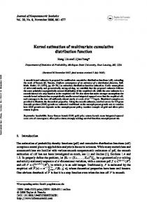
WIND CONDITION DATA The wind data used in this paper is obtained from the North Dakota Agricultural Weather Network (NDAWN) [14]. We use the daily averaged data for wind speed, wind direction, and air temperature measured at the Baker station (Fig. 1) between the year 2000 and 2009. Table 1 shows the geographical coordinates and the elevation of the station. The measurement information is listed as follows.

Multivariate Kernel Density Estimation For a d − variate random sample X1 , X2 , · · · , Xn drawn from a density f , the multivariate KDE is defined to be n

fˆ(x; H) = n−1 ∑ KH (x − Xi )

(3)

i=1

where x = (x1 , x2 , · · · , xd )T and Xi = (Xi1 , Xi2 , · · · , Xid )T , i = 1, 2, · · · , n. Here, K(x) is the kernel that is a symmetric probability density function, H is the bandwidth matrix which is symmetric and positive-definite, and KH (x) = |H|−1/2 K(H −1/2 x). The choice of K is not crucial to the accuracy of kernel density estimators [19]. In this paper, we consider K(x) = ¡ ¢ (2π )−d/2 exp − 21 xT x , the standard normal throughout. In contrast, the choice of H is crucial in determining the performance of fˆ [20].

1. Wind speed is measured at 3 meters above the soil surface with an anemometer. The value is the average of all hourly average wind speeds for a 24-hour period from midnight to midnight. 2. Wind direction is the direction from which wind is blowing (degrees clockwise from north) measured at 3 meters above the soil surface (N = 0◦ ; NE = 45◦ ; E = 90◦ ; SE = 135◦ ; S = 180◦ ; SW = 225◦ ;W = 270◦ ; NW = 315◦ ; etc.) with a wind vane. The value is the average of all measured wind directions for a 24-hour period from midnight to midnight. 3. Air temperature is measured at 1.52 meters above the soil surface with a temperature sensor. The value is the average of the maximum and minimum daily air temperatures.

Optimal Bandwidth Matrix Selection The most commonly used optimality criterion for selecting a bandwidth matrix is the Mean Integrated Squared Error (MISE) [20], which is expressed as MISE(H) = E

Z £

¤2 fˆ(x; H) − f (x) dx

Assuming neutral conditions (negligible thermal effects), the mean velocity in the surface layer (for heights less than 100m) is commonly represented by the log profile [23]. For a known recorded wind speed Um at a height zm , the log profile can be expressed as

(4)

It is usual to employ an asymptotic approximation, known as the AMISE (Asymptotic MISE), which is expressed as

ln zz0 U = zm Um ln z0

1 AMISE(H) = n−1 (4π )−d/2 |H|−1/2 + (vecT H)ψ4 (vecH) (5) 4

where where z0 is the average roughness length (terrain dependent) in the farm region, and U is the wind speed at a height z. The log-profile given by Eq. 8 was used to determine the wind speed at the hub height from the wind speed data recorded at 3m height. The density of dry air can be determined using the ideal gas law, expressed as a function of temperature and pressure [24],

where vec is the vector half operator, given by · vecH = vec

h21 h12

h12 h22

¸



 h21 = h12  h22

The general expression of ψ4 could be found in Wand and Jones [21]. An ideal optimal bandwidth is estimated to be HAMISE = arg min AMISE(H) H

ρ=

(6)

p R×T

(9)

where ρ is the air density, p represents the absolute pressure; R is the specific gas constant for dry air, which is 287.058J/(kg · K), and T represents absolute temperature. The absolute pressure above sea level is given by [24]

In this paper, we use the multivariate plug-in selector (PI(H)) developed by Wand and Jones [22], which is given by 1 PI(H) = n−1 (4π )−d/2 |H|−1/2 + (vecT H)ψˆ 4 (vecH) 4

(8)

³ ´5.25588 p = 101325 1 − 2.25577 × 10−5 × h

(7)

The plug-in estimate of the AMISE can be numerically minimized to give the plug-in bandwidth matrix, Hˆ PI .

(10)

where h is the altitude above sea level. The concerned site in this paper is at an altitude of h = 512m. 3

c 2011 by ASME Copyright °

TABLE 1. DETAILS OF NDAWN STATION: BAKER, ND [14]

Value

Location

Baker, ND

Latitude

48.167◦

Longitude

−99.648◦

Elevation

512m

Histogram MMWD Weibull Gamma Lognormal Normal Rayleigh

0.25

Probability density

Parameter

0.2

0.15

0.1

0.05

0 0

2

4

6

8

10

12

Wind speed (m/s)

FIGURE 2. WIND SPEED PROBABILITY DENSITY FUNCTIONS

FIGURE 1.

errors (MSE) associated with model parameter estimates than MM estimators for large samples considered here [7]. The expressions of the estimated parameters are listed in Appendix A.

BAKER STATION SETUP [14]

MMWD Case I: Univariate Distribution In case I, we are estimating the distribution of the wind speed. Successful modeling of univariate wind speed distribution has been reported in the literature [4,7]. The objective of this case study is to compare the MMWD model with other widely used fitting methods. In this paper, five existing wind distributions are selected, which are Weibull, Gamma, Lognormal, Normal and Rayleigh distributions. The bandwidth h of the KDE is estimated to be 0.6649 using the optimal bandwidth selection method. Figure 2 shows the distribution estimated by the MMWD model and other distribution models. In Fig. 2, the red line represents the wind speed probability distribution estimated by the MMWD model. The cdf, s of the probability distributions are shown in Fig. 3. The goodness-of-fit of the various fitted distributions to the wind speed data is evaluated using the coefficient of determination (R2 ) associated with the resulting Quantile-quantile (Q-Q) plots.

CASE STUDY: APPLICATION OF THE MMWD MODEL The MMWD technique has been applied to three different cases (I, II and III) in order to investigate the extent of wind distribution, as listed below. 1. Case I: Distribution of wind speed (univariate). 2. Case II: Distribution of wind speed and wind direction (bivariate). 3. Case III: Distribution of wind speed, wind direction, and air density (multivariate). In order to validate the effectiveness of the MMWD model, we also investigate and compare the model with standard wind speed distributions [4, 7]: (i) Weibull distribution, (ii) Gamma distribution, (iii) normal distribution, (iv) Lognormal distribution, and (v) Rayleigh distribution. The probability density function (pdf ) and cumulative distribution function (cdf ) of each distribution model are listed in Appendix A. In most of the studies presented in the specialized literature on wind energy and other renewable energy sources, the parameters of the distribution are estimated using classical methods: the method of moments (MM), the maximum likelihood estimators (MLE) and the least squares method (LSM) [25]. The maximum likelihood method has the property of maximizing the value of the probability of the randomly observed sample. MLE is adopted in this paper because it usually yields low mean squared

Quantile-quantile (Q-Q) Plot In statistics, a Q-Q plot is a probability plot, which is a graphical method for comparing two probability distributions by plotting their quantiles against each other [26]. The choice of quantiles from a theoretical distribution has occasioned much discussion. In this paper, we use 4

c 2011 by ASME Copyright °

12

10 0.8

Quantile (Model)

Cumulative distribution function

1

0.6

0.4 MMWD Weibull Gamma Lognormal Normal Rayleigh

0.2

0 0

2

4

6

8

10

8

6 Theoretical MMWD Weibull Gamma Lognormal Normal Rayleigh

4

2

0 0

12

Wind speed (m/s)

2

4

6

8

10

12

Wind speed (m/s)

FIGURE 3. WIND SPEED CUMULATIVE DISTRIBUTION FUNCTIONS

FIGURE 4. WIND SPEED QUANTILE-QUANTILE PLOT OF A SAMPLE OF DATA VERSUS A WEIBULL DISTRIBUTION

dicted) data values, which is expressed as 

the Weibull plotting position [27] in all cases, which is given by

pi = i/(n + 1) where i = 1, 2, · · · , n

R2 =  q

ˆ cov(U, U)

   

(11) =

  

ˆ var(U)var(U)

rh

2 

(12)    

n ∑ni=1 UiUˆ i − ∑ni=1 Ui ∑ni=1 Uˆ i ih ¡ ¢2 i    n ∑ni=1 Ui2 − (∑ni=1 Ui )2 n ∑ni=1 Uˆ i2 − ∑ni=1 Uˆ i

Weibull plotting position always gives an unbiased estimate of the observed cumulative probability regardless of the underlying distribution considered, and does not estimate the highest observed wind speed as the maximum possible wind speed [7]. Figure 4 shows the Q-Q plot of the distributions. The red line is the Q-Q plot of MMWD model. We observe that the MMWD distribution follows the theoretical distribution (45◦ line y = x) closer than other distributions. This observation indicates that the MMWD distribution performs better than other standard distributions for representing the univariate wind speed distribution.

where U and Uˆ are the observed and fitted quantiles; cov and var means covariance and variance, respectively. The closer the value of R2 is to one, the more the fitted distribution agrees with observed data, which indicates a better fit of the model. Table 2 and Fig. 5 show the comparison of the coefficient of determination. It can be seen that, the MMWD model has the largest R2 value. This observation illustrates the strong potential of this technique to provide accurate representation of wind distribution.

Coefficient of Determination The coefficient of determination is a quantity to measure the agreement of a fitting distribution with the recorded data [28]. In the current paper, we evaluate the coefficient of determination between the paired sample quantiles. The coefficient of determination, R2 , is the squared of correlation coefficient between the observed and modeled (pre-

Wind Power Density (WPD) Estimation The WPD expressed in Eqn. (1) is estimated using Monte Carlo integration method based on the pdf of wind speed. Monte Carlo integration is an algorithm for the approximate evaluation of definite integral using random numbers. The sample points for integration in this paper are generated using the Sobol’s quasirandom sequence generator [29]. Sobol sequences use a base of two to form successively finer uniform partitions of the unit interval, and then reorder the coordinates in each dimension. The algo5

c 2011 by ASME Copyright °

TABLE 2.

THE COEFFICIENT OF DETERMINATION, R2

Distribution model

MMWD

Weibull

Gamma

normal

Lognormal

Rayleigh

R2

0.99804

0.98011

0.99796

0.98937

0.95383

0.99511

Square of correlation coefficient, R2

1 0.995 0.99 0.985 0.98 0.975 0.97 0.965 0.96 0.955 0.95

MMWD

Weibull

Gamma Lognormal Normal

Rayleigh

Distribution models

FIGURE 5.

THE COEFFICIENT OF DETERMINATION, R2

FIGURE 8. WIND ROSE AT THREE METERS HEIGHT

rithm for generating Sobol sequences can be found in Bratley and Fox, Algorithm 659 [30]. The approximated WPD is then expressed as

W PD =

Z Umax 1 0 Np

2

Wind Rose A wind rose is a graphical tool used by meteorologists to provide a succinct illustration of how wind speed and wind direction are typically distributed at a particular location. Sixteen cardinal directions are used in this illustration. In this illustration, North corresponds to 0◦ or 360◦ , East to 90◦ , South to 180◦ and West to 270◦ . The cardinal directions are ranked (dc = 1, 2, · · · , 16) in the clockwise order (dc = 1 for North, dc = 5 for East, dc = 9 for South, and dc = 13 for West). Figure 8 shows the estimated wind rose for this location based on the ten-year wind data. We observe that winds from the Northwest and the South dominate over the whole year. Minimal wind is observed from the Northeast direction.

ρ U 3 f (U)dU

1 ' ∑ ρ Ui3 f (Ui )∆U 2 i=1

(13)

where ∆U = Umax /N p where N p is the number of sample size. In this case study, the density of the air is set to a reference value of 1.2kg/m3 at the station. The WPD is then estimated to be 87.83W /m2 based on the ten-year wind data.

Wind Power Density (WPD) Estimation In this case study, the density of the air is also set to a reference value of 1.2kg/m3 . Then, the approximated WPD is expressed as

MMWD Case II: Bivariate Distribution The effectiveness of the MMWD model was validated in case I. Case II investigates the coupled distribution of the wind speed and wind direction. Figures 6(a) and 7(a) represent the estimated wind velocity distribution for the ten-year wind data (2000-2009); Figures 6(b) and 7(b) represent the distribution for the recorded data in the year 2009. Interestingly we observe that the estimated probability distributions are multimodal in nature.

W PD =

Z 360◦ Z Umax 1 0◦ Np

0

2

ρ U 3 f (U, θ )dUd θ

1 ' ∑ ρ Ui3 f (Ui , θi )∆U∆θ i=1 2

(14)

where ∆U∆θ = Umax × 360◦ /N p The WPD is estimated to be 87.83W /m2 . The WPD for each cardinal direction, estimated using the Monte Carlo integration 6

c 2011 by ASME Copyright °

y density Probabilit

y density Probabilit

d in W

d in W

)

e)

e)

re eg (d

re eg (d

s (m/

n io ct

n io ct

re di

re di

d Win

ed spe

(a) ten-year wind data

d Win

ed spe

s (m/

)

(b) year 2009 wind data

FIGURE 6. DISTRIBUTION OF WIND SPEED AND WIND DIRECTION

(a) ten-year wind data

(b) year 2009 wind data

FIGURE 7. DISTRIBUTION OF WIND SPEED AND WIND DIRECTION (CONTOUR PLOT)

method, is shown in Table 3 and Fig. 9. We observe that the wind from northwest has relatively high WPD in this region (as also seen from the wind rose).

MMWD Case III: Multivariate Distribution In case III, we model the multivariate probability distribution of wind speed, wind direction, and air density. It can be seen from Eqn. (1) that the WPD is strongly related to all the three 7

c 2011 by ASME Copyright °

TABLE 3. WPD FOR CARDINAL DIRECTIONS

Direction W PD(W /m2 )

1

2

3

4

5

6

7

8

3.45

4.18

4.20

3.93

3.30

4.13

5.81

6.44

9

10

11

12

13

14

15

16

4.33

2.37

1.69

2.60

5.82

12.72

13.48

7.99

Direction W PD(W /m2 )

14

12

2

WPD (W/m )

10

8

6

4

2

0 0

2

4

6

8

10

12

14

16

Cardinal directions

FIGURE 9.

WPD FOR CARDINAL DIRECTIONS FIGURE 10. DISTRIBUTION OF WIND SPEED, WIND DIRECTION, AND AIR DENSITY

factors. Figure 10 shows the distribution of wind speed, wind direction and air density in a series of nested three-dimensional contours. The contours are at 25% (dark color), 50% (medium color) and 75% (light color), which are upper percentages of highest density regions. A strong correlation among the three wind condition parameters is evident form Fig. 10. This observation is the foundation of our hypothesis - an accurate representation of wind data (for power prediction & farm design) requires multivariate distribution models.

wind data (2000-2009), which is represented by the straight line in Fig. 11. In order to show the variation of wind conditions, the WPD for each single year is evaluated, which is shown in Table 4 and Fig. 11. We can see that the WPD varies significantly over years. The variation is calculated to be 39.24% using Eqn. (16), which indicates significant uncertainty of wind conditions. It is important to recognize that uncertainty anywhere in the system will potentially lead to uncertainty everywhere - thereby eventually impacting the overall power output of the wind farm. Careful modeling and characterization of these uncertainties, together with their propagation into the overall system, will allow for the credible quantification of the overall wind farm power output. Such uncertainty characterization should be an important direction for future research.

Wind Power Density (WPD) Estimation The approximated WPD estimated using Monte Carlo integration method can be expressed as W PD =

Z 360◦ Z Umax Z ρmax 1 0◦

0

ρmin

2

ρ U 3 f (U, θ , ρ )d ρ dUd θ

N

p 1 ' ∑ ρiUi3 f (Ui , θi , ρi )∆U∆θ ∆ρ i=1 2

(15) % variation =

◦

where ∆U∆θ ∆ρ = Umax × 360 × (ρmax − ρmin )/N p

W PDmax −W PDmin W PDavg

(16)

The WPD is estimated to be 84.60W /m2 using the ten-year 8

c 2011 by ASME Copyright °

TABLE 4. WPD FOR EACH SINGLE YEAR

Year

2000

2001

2002

2003

2004

2005

2006

2007

2008

2009

W PD(W /m2 )

80.78

67.31

89.39

77.66

92.64

82.27

84.44

92.37

100.45

67.25

ACKNOWLEDGMENT Support from the National Found Awards CMMI-0533330, CMII-0946765, and CBET-0730922 is gratefully acknowledged.

120 WPD for single year WPD for 10 years (2000−2009)

80

2

WPD (W/m )

100

REFERENCES [1] GWEC, 2008. The global wind 2008 report. Tech. rep., Global Wind Energy Council. [2] Burton, T., Sharpe, D., Jenkins, N., and Bossanyi, E., 2001. Wind energy handbook. Wiley. [3] Manwell, J., McGowan, J., and Rogers, A., 2010. Wind Energy Explained: Theory, Design and Application, 2 ed. Wiley. [4] Carta, J., Ram´ırez, P., and Vel´azquez, S., 2009. “A review of wind speed probability distributions used in wind energy analysis case studies in the canary islands”. Renewable and Sustainable Energy Reviews, 13(5), pp. 933–955. [5] Seguro, J., and Lambert, T., 2000. “Modern estimation of the parameters of the weibull wind speed distribution for wind energy analysis”. Journal of Wind Engineering and Industrial Aerodynamics, 85(1), pp. 75–84. [6] Dorvlo, A., 2002. “Estimating wind speed distribution”. Energy Conversion and Management, 43(17), pp. 2311– 2318. [7] Morgan, E., Lackner, M., Vogel, R., and Baise, L., 2011. “Probability distributions for offshore wind speeds”. Energy Conversion and Management, 52(1), pp. 15–26. [8] Sorensen, P., and Nielsen, T., 2006. “Recalibrating wind turbine wake model parameters - validating the wake model performance for large offshore wind farms”. In European Wind Energy Conference and Exhibition. [9] Katic, I., Hojstrup, J., and Jensen, N., 1986. “A simple model for cluster efficiency”. In Proceedings of European Wind Energy Conference and Exhibition. [10] Lackner, M. A., and Elkinton, C. N., 2007. “An analytical framework for offshore wind farm layout optimization”. Wind Engineering, 31(1), pp. 17–31. [11] Vega, R., 2008. “Wind directionality: A reliability-based approach”. PhD thesis, Texas Tech University, Lubbock, TX, August. [12] Carta, J., Ram´ırez, P., and Bueno, C., 2008. “A joint probability density function of wind speed and direction for wind energy analysis”. Energy Conversion and Management, 49(6), pp. 1309–1320. [13] Erdem, E., and Shi, J., 2011. “Comparison of bivariate distribution construction approaches for analysing wind speed

60

40

20

0

2000 2001 2002 2003 2004 2005 2006 2007 2008 2009

Year

FIGURE 11. WPD FOR EACH SINGLE YEAR (FROM 2000 TO 2009)

CONCLUDING REMARKS AND FUTURE WORK This paper developed a Multivariate and Multimodal Wind Distribution (MMWD) model to represent the distribution of wind conditions (speed, direction and air density) using recorded data. We explored univariate, bivariate and trivariate wind distributions using the MMWD model. The performance of the MMWD model was measured using the coefficient of determination (R2 ) associated with the resulting Quantile-quantile (Q-Q) plots. The effectiveness and the reliability of the MMWD model were successfully validated using the ten-year wind data from the North Dakota Agricultural Weather Network (NDAWN). A strong correlation was observed among wind speed, wind direction, and air density. In addition, the case study illustrated a multimodal wind distribution. These observations corroborate the need to develop wind distribution models that can capture both the multivariate and multimodal nature of recorded data. Such an unassuming stochastic modeling approach can provide a strong foundation to the development of methods to represent the variation in other natural energy resources as well. Specifically, the MMWD model could be helpful for evaluating the wind resource potential for farm siting. The implementation of the MMWD model in optimal planing of commercial scale wind farms should further establish the true potential of this method. 9

c 2011 by ASME Copyright °

expressed as

and direction data”. Wind Energy, 14(1), pp. 27–41. [14] NDAWN, 2010. The north dakota agricultural weather network. http://ndawn.ndsu.nodak.edu/. [15] Simonoff, J., 1996. Smoothing Methods in Statistics, 2 ed. Springer. [16] Rosenblatt, M., 1956. “Remarks on some nonparametric estimates of a density function”. The Annals of Mathematical Statistics, 27(3), pp. 832–837. [17] Parzen, E., 1962. “On estimation of a probability density function and mode”. The Annals of Mathematical Statistics, 33(3), pp. 1065–1076. [18] Jones, M., Marron, J., and Sheather, S., 1996. “A brief survey of bandwidth selection for density estimation”. Journal of the American Statistical Association, 91(433), pp. 401– 407. [19] Epanechnikov, V., 1969. “Non-parametric estimation of a multivariate probability density”. Theory of Probability and its Applications, 14, pp. 153–158. [20] Duong, T., and Hazelton, M., 2003. “Plug-in bandwidth matrices for bivariate kernel density estimation”. Nonparametric Statistics, 15(1), pp. 17–30. [21] M.P. Wand, M. J., 1995. Kernel Smoothing. CRC Press. [22] Wand, W., and Jones, M., 1994. “Multivariate plug-in bandwidth selection”. Computational Statistics, 9, pp. 97–116. [23] Crasto, G., 2007. Numerical simulations of the atmospheric boundary layer. Tech. rep., Universit degli Studi di Cagliari, Cagliari, Italy, February. [24] Kutz, M., 2006. Mechanical engineers’ handbook, 3 ed. Wiley. [25] Canavos, G., 1984. Applied Probability and Statistical Methods. Little, Brown and Company. [26] Gibbons, J., and Chakraborti, S., 2003. Nonparametric Statistical Inference. CRC Press. [27] Looney, S., and Gulledge, T., 1985. “Use of the correlation coefficient with normal probability plots”. The American Statistician, 39(1), pp. 75–79. [28] Forrester, A., S´obester, A., and Keane, A., 2008. Engineering Design via Surrogate Modelling: a Practical Guide. J. Wiley. [29] Sobol, I., 1976. “Uniformly distributed sequences with an additional uniform property”. USSR Computational Mathematics and Mathematical Physics, 16(5), pp. 236–242. [30] Bratley, P., and Fox, B., 1988. “Algorithm 659: Implementing sobol’s quasirandom sequence generator”. ACM Transactions on Mathematical Software, 14(1), pp. 88–100.

f (x; α , β ) =

· ³ ´ ¸ β ³ x ´β −1 x β exp − α α α

(17)

and · ³ ´ ¸ x β F(x; α , β ) = 1 − exp − α

(18)

where x ≥ 0. The estimated shape parameter βˆ can be solved using an iterative procedure, given by 

−1 ³ ˆ ´ β n n x ln x ∑ i 1  i=1 i  βˆ =  − ∑ ln xi  ˆ β n n i=1 ∑i=1 xi

(19)

The estimated scale parameter αˆ can be solved using Ã

αˆ =

1 n βˆ ∑ xi n i=1

!1 βˆ

(20)

Gamma Distribution The Gamma pdf and cdf are expressed as f (x; k, θ ) = xk−1

¡ ¢ exp − θx θ k Γ(k)

(21)

and ¡ ¢ γ k, θx F(x; k, θ ) = Γ(k)

(22)

where x ≥ 0 and k, θ > 0. The estimated parameter kˆ can be obtained by solving à ˆ − ψ (k) ˆ = ln ln(k)

! 1 n 1 n xi − ∑ ln(xi ) ∑ n i=1 n i=1

(23)

ˆ = Γ0 (k)/Γ( ˆ ˆ is the digamma function. The estiwhere ψ (k) k) mated scale parameter θˆ can be solved using

APPENDIX A: PROBABILITY DISTRIBUTION FUNCTIONS Weibull Distribution The 2-parameter Weibull distribution is the most widely accepted distribution for wind speed. The Weibull pdf and cdf are

1 n θˆ = ∑ xi ˆ i=1 kn 10

(24)

c 2011 by ASME Copyright °

Normal Distribution The Normal pdf and cdf are expressed as · ¸ (x − µ )2 exp − 2σ 2 2πσ 2

(25)

· µ ¶¸ 1 x−µ √ 1 + er f 2 σ 2

(26)

f (x; µ , σ ) = √

1

and F(x; µ , σ ) =

The estimated parameter µˆ and σˆ are expressed as

µˆ =

1 n ∑ xi n i=1

and

σˆ =

1 n ∑ (xi − µˆ )2 n i=1

(27)

Lognormal Distribution The Lognormal pdf and cdf are expressed as · ¸ 1 (ln(x) − µL )2 f (x; µL , σL ) = q exp − 2σL2 x 2πσL2

(28)

and F(x; µL , σL ) =

· µ ¶¸ 1 ln(x) − µL √ 1 + er f 2 σL 2

(29)

The estimated parameter µˆL and σˆL are expressed as

µˆL =

1 n ∑ xi n i=1

and

σˆL =

1 n ∑ (xi − µˆL )2 n i=1

(30)

Rayleigh Distribution The Rayleigh pdf and cdf are expressed as µ ¶ x x2 exp − b2 2b2

(31)

¶ µ x2 F(x; b) = 1 − exp − 2 2b

(32)

f (x; b) = and

where x ≥ 0. The estimated parameter bˆ is given by à bˆ =

1 n 2 ∑ xi 2n i=1

!1/2 (33)

11

c 2011 by ASME Copyright °