our multivariate clustering algorithm for large-scale data sets, we take advantage of ... each cluster to the appropriate nodes of the data set's topology tree (where ...... [11] Guha, S., Rastogi, R., Shim, K., Cure: An efficient clustering algorithm for ...
Multivariate Clustering of Large-Scale Scientific Simulation Data Tina Eliassi-Rad
Terence Critchlow
Center for Applied Scientific Computing Lawrence Livermore National Laboratory Box 808, L-560, Livermore, CA 94551 {eliassi, critchlow}@llnl.gov Abstract Simulations of complex scientific phenomena involve the execution of massively parallel computer programs. These simulation programs generate large-scale data sets over the spatio-temporal space. Modeling such massive data sets is an essential step in helping scientists discover new information from their computer simulations. In this paper, we present a simple but effective multivariate clustering algorithm for large-scale scientific simulation data sets. Our algorithm utilizes the cosine similarity measure to cluster the field variables in a data set. Field variables include all variables except the spatial (x, y, z) and temporal (time) variables. The exclusion of the spatial dimensions is important since “similar” characteristics could be located (spatially) far from each other. To scale our multivariate clustering algorithm for large-scale data sets, we take advantage of the geometrical properties of the cosine similarity measure. This allows us to reduce the modeling time from O(n2) to O(n × g(f(u))), where n is the number of data points, f(u) is a function of the user-defined clustering threshold, and g(f(u)) is the number of data points satisfying f(u). We show that on average g(f(u)) is much less than n. Finally, even though spatial variables do not play a role in building clusters, it is desirable to associate each cluster with its correct spatial region. To achieve this, we present a linking algorithm for connecting each cluster to the appropriate nodes of the data set’s topology tree (where the spatial information of the data set is stored). Our experimental evaluations on two largescale simulation data sets illustrate the value of our multivariate clustering and linking algorithms.
1. Introduction Scientists are able to simulate complex phenomena by utilizing massively parallel computer programs. Such computer programs (a.k.a., simulation codes) produce terascale data sets over the spatio-temporal space. In order to discover new information from such large-scale data sets, scientists need efficient and effective modeling techniques [1, 6, 8, 14]. This paper describes a simple yet effective multivariate clustering algorithm for large-scale scientific simulation data in mesh format. Mesh data sets usually
vary with time, consist of multiple dimensions (i.e., variables), and contain interconnected grids. Such grids break the mesh data into zones, in which data points are stored. The shape of the zones can be regular (e.g., rectilinear) or irregular (e.g., arbitrary polygons). Figure 1 depicts part of the mesh produced from an astrophysics simulation of a star exploding. Musick and Critchlow provide a nice introduction to scientific mesh data [15].
Figure 1. Part of a Mesh Data Set Representing the Explosion of a Star Our multivariate clustering algorithm uses only a data set’s field variables to find “similar” behavior. Field variables are all variables except the spatial (x, y, z) and temporal (time) variables. For example, temperature, pressure, and density are considered field variables. The exclusion of the spatial dimensions from the clustering process is important since “similar” characteristics could be far from each other in the spatial region (see Figure 2). For example, the values of the field variables in the outer zones of a star are homogeneous even though spatially the zones can be far apart. To build clusters, we utilize a variant of the cosine similarity measure, which has been used in information retrieval applications [17]. We chose the cosine similarity measure instead of other metrics (such as the Euclidean distance metric) since our clusters will be used for query retrieval.
2. Multivariate Clustering
Figure 2. A Mesh Data Set Representing a Star (Similar Zones Have Similar Colors.) To scale our multivariate clustering algorithm for largescale data sets, we take advantage of the geometrical properties of the cosine similarity measure. Specifically, we utilize the user-defined clustering threshold to place a tighter upper-bound on the similarity of zones. This allows us to reduce the clustering time from O(n2) to O(n × g(f(u))), where n is the number of data points, f(u) is a function of the user-defined clustering threshold, and g(f(u)) is the number of data points satisfying the new threshold f(u). We empirically show that on average g(f(u)) is much less than n. Section 2 describes our multivariate clustering algorithm in details. Even though spatial variables do not play a role in building our clusters, it is desirable to associate each cluster with its correct spatial region. In particular, it is important for our clustering model to frame the answers to scientists’ queries in the spatial location of the original data. To achieve this, we present a linking algorithm for connecting each cluster to the appropriate nodes of the data set’s topology tree. Such a tree stores the spatial information of a data set by utilizing the intrinsic topology of the data given in the original scientific problem [5]. Our linking technique is embedded into our clustering algorithm. That is, connections between a cluster and the correct nodes of the topology tree are made as the cluster is being constructed. In this way, we are able to avoid traversing the clusters after they are made, which in turn reduces our execution times. The main challenge for our linking algorithm is to find the best m nodes in the topology tree for a particular cluster, c, where m is much less then the number of zones in c. Section 3 presents an in-depth discussion of our linking algorithm. In Section 4, we describe our experimental evaluations on two large-scale (astrophysics) simulation data sets. We compare our results with a simple modeling technique, which propagates statistical information of the data up the topology tree. Our results illustrate the value of our multivariate clustering and linking algorithms. Sections 5 and 6 discuss some related and future works, respectively. Finally, Section 7 provides a summary of our work.
Our motivation for using a multivariate modeling algorithm is to capture the interrelationships among a mesh data set’s field variables in one metric. In this way, we are able to collectively measure the similarity between zones. Eliassi-Rad, et al [8] presents our work using univariate modeling algorithms. Table 1 describes our multivariate clustering algorithm. The inputs to our algorithm are (i) the list of zones in the mesh data set and (ii) a user-defined clustering threshold in [0,1]. A clustering threshold of 0 indicates complete dissimilarity between zones. On the other hand, a clustering threshold of 1 shows total similarity among zones. The output of our algorithm is a list of clusters, where each cluster is represented by its (zone) population, N, and the following four vectors: 1 2 = � m
1 2 = � m →
→
→
max1 max2 max = � maxm
min1 min2 min = � minm
→
, , max , and min are the mean, standard deviation, maximum, and minimum values of the zones represented in a cluster. The variable m is the number of field variables in the mesh data set. Initially, we assume that all zones are available for clustering (i.e., they are assigned the color GREEN). Then, as each zone is placed in an appropriate cluster, it becomes unavailable (i.e., its color changes from GREEN to RED). Our clustering algorithm iterates over all GREEN zones. At each iteration, a variant of the cosine similarity measure [17] is used to find an appropriate cluster for each GREEN zone. Table 1. Our Multivariate Clustering Algorithm Inputs List of zones User-defined clustering threshold in [0, 1], where 0 and 1 indicate complete dissimilarity and similarity, respectively. Output A list of clusters Assumptions A zone is either GREEN (i.e., available for clustering) or RED (i.e., already included in a cluster). Initially, the color of all zones, z, is GREEN.
Algorithm For each zone, z, do If (z.color GREEN) then a) C = new Cluster(); b) Add z to C; c) C.stats = z.stats; d) z.color = RED; e) For each zone, z , do i) If (z .color GREEN) then (1) If (CosSim(z, z ) �f(u)) then (a) Add z to C; (b) Update C.stats; (c) z .color = RED; f) Add C to the list of clusters; The standard cosine similarity measure between two & & vectors and is defined as follows: & & & & & & • & , if ≠ 0 and ≠ 0 cos( , ) = & × 2 2 & & & & CosSim( , ) = 1, if = & & & & 0, if ( = 0 & ≠ 0) or ( ≠ 0 & = 0) Since we cluster the zones of a mesh data, we need to represent each zone as a vector. The vector associated with each zone contains the mean values of the field data points & in that zone. Our CosSim normalizes the elements of
[0,1] to [-1,1].1 In particular, we use the following equation to do this mapping: new_user_threshold = (2 × user_threshold) – 1 Then, we define our new threshold, f(u), to be: f(u) = f(new_user_threshold) = cos(0.5 × (cos-1(new_user_threshold))) Based on the geometrical properties of the cosine function, the new_user_threshold is always less than f(u). So, we can use the following inequality: new_user_threshold < f(u) CosSim(z, z ) Moreover, we are guaranteed that any new zone added to a cluster, C, satisfies the user-defined similarity measure. Figure 3 pictorially illustrates this fact. Based on the user’ s & & threshold, any two vectors and are considered similar & & if and only if the cosine of the angle between and is greater than or equal to new_user_threshold. In our clustering algorithm, if the angle between an arbitrary & vector and any vector in a cluster C, is half the size of & & & the angle between and , then is safely added to the cluster C (without any additional pair-wise comparisons).
& User-Defined Threshold = cos-1(new_user_threshold) & Our Threshold =0.5 × cos-1(new_user_threshold)
&
and such that all the values of field variables are between 0 and 1. This normalization step is important since the ranges of values for our field variables differ considerably. & & Traditionally, when CosSim ( , ) user_threshold is & & true, and are placed into one cluster. Then, a new & & & vector, , is placed in the same cluster as and only if both of the following inequalities are true: & & • CosSim ( , ) �user_threshold, and & & • CosSim ( , ) �user_threshold Since we have a huge number of zones to process, calculations of all pair-wise CosSim measures can be quite burdensome. Furthermore, sampling from the mesh data is not an option since scientists are interested in outliers and do not tolerate results from sampled data. Therefore, we tighten the similarity threshold so as to eliminate the need to compute all the pair-wise comparisons. In particular, each new GREEN zone is only compared with the first zone that was added to the cluster. We get our new threshold by first mapping the user-defined threshold from
& Figure 3. User-Defined Threshold and Our Threshold The tightening of the similarity threshold helps us in two ways. First, we do not spend time on pair-wise comparisons. Second, we do not need to shuffle zones between clusters since our bound, f(u), eliminates zones that are on the cluster boundaries. In the best case, our clustering algorithm runs in O(n) time, where n is the number of zones in the mesh data sets. In the worst case, our algorithm runs in O(n2) time. However, on average, our algorithm runs in O(n × g(f(u))) times, where g(f(u)) is the number of zones that satisfy the f(u) bound. In our experimental results reported in Section 4, g(f(u)) is much less than n.
1
The original user-defined threshold is in [0,1] (and not [1,1]) since it is easier for users to think in terms of the interval [0,1].
3. Cluster-Topology Linking Even though spatial variables do not play a role in building clusters in our algorithm, it is desirable to associate each cluster with its correct spatial region. In particular, it is important for our clustering model to return answers to scientists’ queries in the spatial region of the original mesh. Since our mesh data have millions of zones, it would be very inefficient (and at times impossible) to link each cluster with all of its zones. Therefore, we present a linking algorithm for connecting each cluster to a small set (e.g., 512) of nodes in the data set’ s topology tree. A topology tree stores the spatial information of a data set by utilizing the intrinsic topology of the data given in the original scientific problem [5]. Figure 4 illustrates a topology tree, where the zones are agglomerated topologically to create interior cells. Then, the interior cells are recursively agglomerated based on their topology until one only one cell (i.e., root cell) remains.
z, then that link’ s percentage_intersection is 100. This percentage_intersection metric measures the “ quality” of a link. A threshold can be placed on the percentage_intersection metric so that the trade-off between execution time and links to the best-fitting nodes can be exploited.
Root Cell
… Link
…
…
Interior Cells
…
Link Cluster A
…
…
…
Root Cell
…
…
Cluster … B
Zones
Link List of Clusters
… Interior Cells Zones
Figure 4. A Topology Tree Figure 5 shows sample links between the list of clusters and the topology tree. Our linking technique is embedded into our clustering algorithm. That is, connections between a cluster and the correct nodes of the topology tree are made as the cluster is being constructed. In this way, we are able to avoid traversing the clusters after they are made, which in turn reduces our execution times. The main challenge for our linking algorithm is to find the “ best” k nodes in the topology tree for a particular cluster, C, where k (e.g., 512) is much less then the number of zones in C (e.g., 1,625,000). Table 2 describes our linking algorithm. When the list of links for a cluster is full, we traverse the topology and the list of links to find the lowest level topology node with the most number of descendents in the list of links. Each link between a cluster and a tree node has a metric, called percentage_intersection, which measures the percentage intersection between the zones in the clusters and the descendents of a node. For example, if a zone, z, is in cluster C and the list of links for C has a link connected to
Figure 5. Links Between List of Clusters and Topology Tree
Table 2. Our Linking Algorithm Input links = list of links for cluster, C z = zone being added to C Output Update links Algorithm If (links is not full) then • z.percentage_intersection = 100; • Add z to links; • Return links; Else • For l = 0 (leaf level) to r (root level), do (1) z.ancestor[l] = z’ s ancestor at l; (2) If (z.ancestor[l] is in links) then update z.ancestor[l].percentage_intersection; (3) Return links; • new_link = NULL; • For each link, j, in links, do (1) best_ancestor[j] = j’ s ancestor with the most number of descendents in links;
• • • • •
(2) If (best_ancestor[j].num_descendents � MAX_NUM_DESCENDENTS) then (a) new_link = best_ancestor[j]; (b) break; If (new_link NULL) then (1) new_link = argmaxj∈ links best_ancestor[j]; Clear all descendents of new_link from links; Set new_link.percentage_intersection; Add new_link to links; Return links;
o Execution time for building clusters with and without the linking algorithm • Maximum level reached when linking clusters to topology tree • Minimum percentage_intersection at the maximum level reached • Maximum percentage_intersection at the maximum level reached
Our linking algorithm performs quite well. This is due to the very small number of levels in a topology tree (usually less than 20) and the small number of links chosen to connect a cluster to the topology tree (usually less than 1000).
4. Experimental Evaluations Our experiments describe the performance of our multivariate clustering algorithm with and without the linking algorithm on two large-scale simulation data sets. We also compare these performances to the topology-based algorithm, where the statistical information of the field variables is propagated upwards in the tree [5].
Figure 6. The White-Dwarf Data Set
4.1 Data Sets Table 3 describes the two mesh data sets used in our experiments. Both data sets are a simulation of a star at a certain stage of its life and represent readings in point locations of a continuous medium. The data sets are represented as zones (i.e., small cubes with 8 nodes). Values of variables are associated either with each node (called a nodal variable) or with each zone (called a zonal variable). The White Dwarf data set (see Figure 6) is a simulation of a star exploding. The Djehuty data set (see Figure 7) is a simulation of a star at its mid-life. Table 3. Characteristics of Our Data Sets Data Set
# of Zones
# of Variables
# of Time Steps
White Dwarf
557,375
20
22
Djehuty
1,625,000
18
16
4.2 Evaluation Metrics We compare our different algorithms by using the following evaluation metrics in our experiments: • Metrics per time step o Number of clusters created o Average number of zones in clusters o Minimum number of zones in clusters o Maximum number of zones in clusters
Figure 7. The Djehuty Data Set
4.3 Results Tables 4 and 5 list the results of our clustering algorithm without linking and with a user_threshold of 0.95 (in [0,1]). An intuitive way of thinking about the user_threshold is to state that the user requires all zones in a cluster to be (user_threshold × 100) percent similar. So, when user_threshold is 0.95, the required similarity between zones in a cluster is 95%. Our threshold tightens this percentage to 98% similarity between zones in a cluster. Note the small number of clusters that we are able to build from hundreds of thousands of zones. It is also interesting to point out that for the White Dwarf data set when the star starts exploding at time step = 1, the number of clusters increases by a factor of 7.5. On the other hand, since a major event does not occur in the Djehuty data set, there is
no dramatic increase in number of clusters from one time step to the next. This behavior is also evident in the minimum, average, and maximum number of zones in clusters (per time step). Table 4. Clustering on White Dwarf (user_thresold = 95% and f(u) = 98.5%)
Time Step
Execution Time Without Linking in Seconds
0 1 2 3 4 5 6 7 8 9 10 11 12 13 14 15 16 17 18 19 20 21
86.21 204.79 136.87 179.61 121.79 158.31 146.58 119.34 124.15 129.85 142.95 94.02 131.17 143.77 193.21 150.41 149.58 125.67 140.69 78.48 144.29 154.90
# of Clusters Made from 557,375 Zones 13 98 31 30 32 32 43 41 42 42 47 33 35 32 43 45 41 41 42 34 34 30
Min # of Zones in Clusters
Avg # of Zones in Clusters
Max # of Zones in Clusters
8121 1 4 6 9 1 1 5 7 7 3 2 3 4 1 1 40 40 8 3 2 19
42875.0 5687.5 17979.8 18579.2 17418.0 17418.0 12962.2 13594.5 13270.8 13270.8 11859.0 16890.2 15925.0 17418.0 12962.2 12386.1 13594.5 13594.5 13270.8 16393.4 16393.4 18579.2
110250 136682 186088 151369 150325 149505 143488 136427 133933 133219 116237 167776 176328 217124 171179 170608 170230 169933 132618 226312 226523 235491
Tables 6 and 7 list the results of our clustering algorithm without linking and with a user_thresold of 0.99 (in [0, 1]). The bound used by our clustering algorithm is 0.995 in [-1, 1] (which is equivalent to 99.75% similarity within each cluster). Again, there is a dramatic increase (by a factor of 36.75) in the number of cluster made for the White Dwarf data set from time step = 0 to time step = 1 (because of the start of explosion in the star). As expected, the execution times are also longer with the bound of 99.75% similarity as opposed to a bound of 98.5% similarity. Table 5. Clustering on Djehuty (user_thresold = 95% and f(u) = 98.5%)
Time Step
0 1
Execution Time Without Linking in Seconds 578.95 562.46
# of Clusters Made from 1,625,000 Zones 14 16
Min # of Zones in Clusters
Avg # of Zones in Clusters
Max # of Zones in Clusters
4 8
116071 101563
387420 379529
2 3 4 5 6 7 8 9 10 11 12 13 14 15
763.35 800.39 692.21 532.98 543.35 542.96 536.54 538.26 529.28 541.39 528.73 527.83 519.78 531.86
27 46 50 49 50 53 50 52 50 48 48 48 48 48
135 96 6 36 12 1 13 4 39 196 1 102 18 3
60185.2 35326.0 32500.0 33163.3 32500.0 30660.4 32500.0 31250.0 32500.0 33854.2 33854.2 33854.2 33854.2 33854.2
383366 385078 378161 413040 420249 421951 423756 424303 423165 420973 419518 416561 414733 412607
Table 6. Clustering on White Dwarf (user_thresold = 99% and f(u) = 99.75%)
Time Step
Execution Time Without Linking in Seconds
0 1 2 3 4 5 6 7 8 9
94.10 1259.80 622.99 361.91 323.89 384.50 1750.70 2830.02 3330.36 4727.93
# of Clusters Made from 557,375 Zones 28 1029 195 201 187 178 232 251 250 262
Min # of Zones in Clusters
Avg # of Zones in Clusters
Max # of Zones in Clusters
2801 1 1 1 1 1 1 1 1 1
19906.3 541.7 2858.3 2773.0 2980.6 3131.32 2402.5 2220.6 2229.5 2127.39
58800 88947 66281 49470 48781 45454 68549 44835 43742 43486
Table 7. Clustering on Djehuty (user_thresold = 99% and f(u) = 99.75%)
Time Step
0 1 2 3 4 5 6 7 8 9 10 11 12 13 14 15
Execution Time Without Linking in Seconds 939.44 1148.61 1650.27 2288.11 3382.61 4047.15 3612.45 3924.49 3480.74 3089.25 4928.18 6628.21 7688.57 8484.75 10922.2 11319.7
# of Clusters Made from 1,625,000 Zones 101 152 288 511 628 633 639 651 657 641 635 620 627 605 597 594
Min # of Zones in Clusters
Avg # of Zones in Clusters
Max # of Zones in Clusters
2 4 1 3 1 1 2 1 1 2 2 1 1 2 1 1
16089.1 10690.8 5642.36 3180.04 2587.58 2567.14 2543.04 2496.16 2473.36 2535.10 2559.06 2620.97 2591.71 2685.95 2721.94 2735.69
360000 351174 311071 271924 288192 236610 285632 315302 320345 311419 298567 262135 191985 169082 163168 151338
Tables 8 and 9 show the execution times of our clustering algorithm with and without linking on the first six time steps of White Dwarf and Djehuty, respectively. In addition, they list the best and worst quality of links made between clusters and the topology tree. As expected, it takes longer to build clusters and connect them to the topology tree. However, the most increase is by a factor of 5.6 (see time step = 0 in Table 8). Both the White Dwarf and the Djehuty topology trees have a maximum of 11 levels. The highest level in the tree reached for a connection between a cluster and a node is 4 and 5 for White Dwarf and Djehuty, respectively. This is quite good since a link accessing a high tree level usually has a worse fit (i.e., percentage_intersection) as compared to a link connecting to a lower tree level. Even so, in both data sets, the maximum percentage_intersection at the highest level is 100% for both data sets. That is, for the Djehuty data set, there are nodes at level 5 which contain all the zones in a cluster. The minimum percentage_intersection at the highest level is 25% and 12.5% for White Dwarf and Djehuty, respectively. This minimum percentage_intersection value shows the quality of the worst links. For example, in the Djehuty data set, there are nodes at level 5 which contain only 12.5% of the zones in a cluster. Table 10 illustrates the execution times of our multivariate clustering algorithm (without linking). As was expected, the average value of g(f(u)), which is the number of zones satisfying our threshold f(u), is much less than n (the total number of zones). In fact, the average g(f(u)) is in single digits while the average n is in hundreds of thousands. Table 8. Clustering on White Dwarf (user_thresold = 99% and f(u) = 99.75%)
0 1 2 3 4 5 Max Level Reached in Topology Tree
Execution Time Without Linking in Seconds 94.10 1259.80 622.99 361.91 323.89 384.50 Max Level Reached with Linking
11
4
Time Step
Execution Time With Linking in Seconds 867.24 1489.42 763.51 712.41 672.48 753.06 Min and Max % intersection at Max Level Min = 25% and Max = 100%
Table 9. Clustering on Djehuty (user_thresold = 99% and f(u) = 99.75%) Time Step 0 1 2 3 4 5 Max Level in Topology Tree 11
Execution Time Without Linking in Seconds 939.44 1148.61 1650.27 2288.11 3382.61 4047.15 Max Level Reached with Linking 5
Execution Time With Linking in Seconds 2467.04 2569.44 2926.92 3524.46 4828.16 5597.04 Min and Max % intersection at Max Level Min = 12.5% and Max = 100%
Table 10. Execution Times for Our Multivariate Clustering Algorithm (without Linking) and Average Value for g(f(u)) Data Set
User Threshold
Avg O(n) in Seconds
Avg O(n × g(f(u))) in Seconds
Avg g(f(u))
White Dwarf
95%
232.32
732.09
3.15
White Dwarf
99%
281.33
2179.6
7.75
Djehuty
95%
351.22
1249.6
3.56
Djehuty
99%
763.91
1587.1
2.08
Tables 11 and 12 compare our clustering algorithm with linking to the topology-based agglomeration algorithm (which produces the topology tree). The number of nodes made by the topology-based agglomeration algorithm (in one level) is much larger than the number of clusters made by our clustering algorithm. This is mostly due to the design of the topology-based agglomeration algorithm, which combines no more than eight zones at a time. This strategy of agglomerating only small number of zones based solely on their topology also makes the topology-based agglomeration algorithm run faster than our clustering algorithm. In short, Tables 11 and 12 show how well our clustering algorithm is able to agglomerate “ similar” zones.
Table 11. White Dwarf Data Set: Comparison of Our Multivariate Clustering Algorithm (with Linking) Versus the Topology-Based Agglomeration Data Set = White Dwarf Time Step = 0 User Threshold = 99%
Execution Time in Seconds
Number of Agglomerations Made from 557,375 Zones
Topology-Based Agglomeration Algorithm
753.44
73924
Multivariate Clustering with Linking
867.24
28
Table 12. Djehuty Data Set: Comparison of Our Multivariate Clustering Algorithm (with Linking) Versus the Topology-Based Agglomeration Data Set = Djehuty Time Step = 0 User Threshold = 99%
Execution Time in Seconds
Number of Agglomerations Made from 1,625,000 Zones
Topology-Based Agglomeration Algorithm
946.57
203125
Multivariate Clustering with Linking
2467.04
101
5. Related Work Clustering algorithm such as BIRCH [20], CHAMELEON [13], CLARANS [16], CLIQUE [3], CURE [11], and DBSCAN [9] cannot be either used or scaled to our data sets for one or more of the following reasons: 1. Our modeling techniques cannot require sampling. Scientists already sample the data produced by their simulation programs. They do not accept models that sample the sampled data, particularly since they are mostly interested in outliers. 2. We can not build clusters from zones in a subspace of the data since global properties are important. 3. It is not desirable to use binning or histograms techniques since we are not supposed to assume an a priori distribution on the data. Moreover, histograms are computationally expensive on highdimensional data sets. Our work is similar to Freitag and Loy [10]. Their system builds distributed octrees from large scientific data sets. They, however, reduce their data by constraining the points to their spatial locations. STING [19] is also similar to our work except that it assumes that the distribution of the data is known. Also, it has been tested only on small data sets containing only tens of thousands of data points. DuMouchel, et al [7] present a method for compressing flat files; however, they use binning techniques to “ squash” files, which impose an a
priori distribution on the data Finally, AQUA [2] uses cached summary data in an OLAP domain. They also use sampling and histogram techniques, which are not acceptable in our models.
6. Current and Future Work We are extending our algorithm to capture “ similar” behavior across time steps. In particular, we would like to build a cluster hierarchy from the clusters made at each time step. We conjecture that such hierarchies will speedup response times for queries on both the clusters and the topology tree since the cluster hierarchy will be shallow with manageable number of links to the topology tree. Moreover, we plan to develop tools, which track a particular zone across time steps. Such tools will not only help scientists’ in their queries but also will provide us with insight into our clustering algorithm. We are examining other measures of interest to see how they compare to the normalized cosine similarity measure [12, 18]. In addition, we are looking into ways in which the inputted list of zones is efficiently perturbed before each clustering step. Finally, we are investigating other modeling techniques for large-scale simulation data sets [4]. Specifically, we are interested in models that (i) require only one sweep of data, (ii) are good at finding outliers, (iii) can be easily parallelized, and (iv) can efficiently answer a wide variety of queries.
7. Conclusion Massively parallel computer programs (which simulate complex scientific phenomena) generate large-scale data sets over the spatio-temporal space. Modeling such massive data sets is an essential step in helping scientists discover new information from these computer simulations. We present a simple but effective multivariate clustering algorithm for large-scale scientific simulation data sets. Our algorithm utilizes the cosine similarity measure to cluster the field variables in a data set. The exclusion of the spatial location is important since “ similar” characteristics could be located (spatially) far from each other. To scale our multivariate clustering algorithm for large-scale data sets, we take advantage of the geometrical properties of the cosine similarity measure. This allows us to reduce the modeling time from O(n2) to O(n × g(f(u))), where n is the number of data points, f(u) is a function of the user-defined clustering threshold, and g(f(u)) is the number of data points satisfying the threshold f(u). We show that on average g(f(u)) is much less than n. Finally, even though spatial variables do not play a role in building a cluster, it is desirable to associate each cluster with its correct spatial location. To achieve this, we present a linking algorithm for connecting each cluster to the appropriate nodes of the data set’ s topology tree. Our experimental evaluations on
two large-scale astro-physics simulation data sets illustrate the value of our multivariate clustering and linking algorithms.
[9] Ester, M., Kriegel, H.-P., Sander, J., and Xu, X., A density-based algorithm for discovering clusters in large spatial databases with noise, In Proceedings of KDD 1996 (Portland OR, August 1996), 226-231.
8. Acknowledgments
[10] Freitag, L.A., and Loy, R.M. Adaptive, multiresolution visualization of large data sets using a distributed memory octree, In Proceedings of SC 1999 (Portland OR, November 1999), ACM Press, Article 60.
This work was performed under the auspices of the U.S. Department of Energy by the University of California Lawrence Livermore National Laboratory under contract No. W-7405-ENG-48.1. UCRL-JC-151860-REV-1. Our thanks to Ghaleb Abdulla, Bill Arrighi, Chuck Baldwin, Kevin Durrenberger, Nu Ai Tang, and Megan Thomas for their assistance.
9. References [1] Abdulla, G., Baldwin, C., Critchlow, T., Kamimura, R., Lozares, I., Musick, R., Tang, N.A., Lee, B., and Snapp, R. Approximate ad-hoc query engine for simulation data, In Proceedings of JCDL 2001 (Roanoke VA, June 2001), ACM Press, 255-256. [2] Acharya, S., Gibbsons, P.B., Poosala, V., and Ramaswamy, S. The Aqua approximate query answering system, In Proceedings of the 1999 ACM SIGMOD, ACM Press, 574-576. [3] Agrawal, R., Gehrke, J., Gunopulos, D., Raghavan, P., Automatic subspace clustering of high dimensional data for data mining applications, In Proceedings of SIDMOD 1998 (June 1998), ACM Press, 94-105. [4] Baldwin, C., Abdulla, G., and Critchlow, T. MultiResolution Modeling of Large Scale Scientific Simulation Data, LLNL Technical Report, UCRL-JC147225, 2003. [5] Baldwin, C., Eliassi-Rad, T., Adbulla, G., and Critchlow, T., The evolution of a hierarchical partitioning algorithm for large-scale scientific data: three steps of increasing complexity, In Proceedings of SSDBM 2003 (July 2003). [6] Chakrabarti, K., Garofalakis, M., Rastogi, R., and Shim, K. Approximate query processing using wavelets, In Proceedings of VLDB 2000 (Cairo Egypt, September 2000), ACM Press, 111-122.
[11] Guha, S., Rastogi, R., Shim, K., Cure: An efficient clustering algorithm for large databases, In Proceedings of SIGMOD 1998 (Seattle WA), ACM Press, 73-84. [12] Hilderman, R.J., and Hamilton, H.J., Knowledge Discovery and Measures of Interest, Kluwer Academic Publishers, Boston, MA, 2001. [13] Karypis, G., Han, E.-H., Kumar, V., Chameleon: Hierarchical clustering using dynamic modeling, IEEE Computer (August 1999), 68-75. [14] Lee, B., Critchlow, T., Abdulla, G., Baldwin, C., Kamimura, R., Musick, R., Snapp, R., and Tang, N.A., The framework for approximate queries on simulation data, International Journal of Information Sciences, Elsevier Sciences, forthcoming. [15] Musick, R., and Critchlow, T. Practical lessons in supporting large-scale computational science, In Proceedings of SIGMOD Record 1999, ACM Press, 28(4):49-57. [16] Ng, R.T., and Han, J., Efficient and effective clustering methods for spatial data mining, In Proceedings of VLDB 1994 (Santiago Chile, September 1994), Morgan Kaufmann Publisher, 144-155. [17] Van Rijsbergen, C.J., Information Retrieval, 2nd edition, Butterworths, London, UK, 1979. [18] Wang, J., Wang, X., Lin, K.-I., Shasha, D., Shapiro, B.A., Zhang, K., Evaluating a class of distancemapping algorithms for data mining and clustering, In Proceedings of KDD 1999 (San Diego CA), ACM Press, 307-311.
[7] DuMouchel, W., Volinsky, CH., Johnson, T., Cortes, C., and Pregibon, D., Squashing flat files flatter, In KDD 1999 (San Diego CA), ACM Press, 6-15
[19] Wang, W., Yang, J., and Muntz, R. STING: A statistical information grid approach to spatial data mining, In Proceedings of VLDB 1997 (Athens Greece, August 1997), Morgan Kaufmann Publishers, 186-195.
[8] Eliassi-Rad, T., Critchlow, T., and Abdulla, G., Statistical modeling of large-scale simulation data, In Proceedings of ACM SIGKDD 2002 (Edmonton Canada, July 2002), ACM Press, 488-494.
[20] Zhang, T., Ramakrishnan, R., and Livny, M., BIRCH: An efficient data clustering method for very large databases, In Proceedings of SIGMOD 1996 (June 1996), ACM Press, 103-114.