To appear in the proceedings of the BISC FLINT-CIBI 2003 workshop, Berkeley, Dec. 2003.
Multivariate Non-Linear Feature Selection with Kernel Multiplicative Updates and Gram-Schmidt Relief
Isabelle Guyon Clopinet, 955 Creston Road, Berkeley, CA94708,
[email protected] and Hans-Marcus Bitter, Zulfikar Ahmed, Michael Brown, and Jonathan Heller Biospect, 201 Gateway Blvd, So. San Francisco, CA 94080
We address problems of classification in which the number of input components (variables, features) is very large compared to the number of training samples. In this setting, it is often desirable to perform a feature selection to reduce the number of inputs, either for efficiency, performance, or to gain understanding of the data and the classifiers. We compare a number of methods on mass-spectrometric data of human protein sera from asymptomatic patients and prostate cancer patients. We show empirical evidence that, in spite of the high danger of overfitting, non-linear methods can outperform linear methods, both in performance and number of features selected.
1 Background on the Problem of Feature Selection The problem of variable and feature selection has been tackled from many perspectives. For a review, see (Guyon and Elisseeff 2003) and references therein. This problem has recently attracted a lot of attention because new application domains produce data with huge numbers of features (10,000, 100,000, or even millions), e.g. in bioinformatics for the study of the genome and the proteome, in pharmacology for high throughput drug screening, and in text processing. A recent benchmark that we have organized presents results on a variety of datasets (http://clopinet.com/isabelle/Projects/NIPS2003/). We limit ourselves here to presenting some basic notions that outline the need for non-linear multivariate feature selection. A first set of methods that are commonly used in bioinformatics and text processing consist in ranking features according to their individual predictive power. Such techniques include correlation methods, T-test, Fisher score, etc. A state-of-the art version of this generic approach has been proposed recently by (Tibshirani et al 2002). We refer to such methods as “linear univariate” because they make a convex combination of linear classifiers that are built using single variables. While it is also possible to use “non-linear univariate” methods, we do not consider these in this study because they are rarely used, particularly in our application domain. A second set of methods, which we investigate, are “linear multivariate” and make use of linear discriminant classifiers. Such classifiers are built with a subset of features. They are used to score feature subsets, according to classification performance.
1
To appear in the proceedings of the BISC FLINT-CIBI 2003 workshop, Berkeley, Dec. 2003.
Finally, a third set of methods use non-linear discriminant classifiers to perform the same task. We refer to those as “non-linear multivariate”. It is common in the literature to make the distinction between “filters” and “wrappers” for feature selection. However, this distinction is not relevant to our study. Filters are methods that select features without the direct goal of optimizing the performance of a particular classifier. The resulting features are used with any classifier. Wrappers and embedded methods are directly tied to a given classifier: they use the performance of the classifier (or a prediction of its performance) to select subsets of features, eventually conducting a search in the space of all possible feature subsets. In this study, we make use of a filter (the shrunken centroid method) that can be considered a wrapper if the input statistical independence assumptions are actually verified. Conversely, we use wrappers as filters to select features for other methods. Table 1. Color coding for method attribute combinations. Linear univariate Non-linear univariate
Linear multivariate Non-linear multivariate
In our tutorial (Guyon and Elisseff 2003), we have shown simple examples of problems that are inherently multivariate and cannot be solved with univariate techniques: the data separation lies in a subspace of dimension greater than one. We have shown cases in which a particular feature taken alone carries no class-separation power, yet it can improve classification performance when taken together with another one. Additionally, some problems have strong non-linearities. The optimum non-linear decision surface may lie in a multi-dimensional subspace. We have seen examples in which two (or more) features that individually carry no class-separation power can improve classification performance when considered simultaneously. Table 1 summarizes the various cases under consideration. Even though multivariate methods lead to more universal predictors than univariate methods and non-linear methods more universal predictors than linear methods, they may turn out to provide poorer performance. This is due to the problem of overfitting. In large dimensional spaces, with the availability of a small number of training examples, being able to learn a broader class of functions is often synonymous to providing poor generalization capabilities on test data (distinct from the training data). For a theoretical treatment of this problem, see e.g. (Vapnik 1998). The purpose of this paper is to see whether pessimistic theoretical predictions hold in practice. We show in this study that in fact they don’t: non-linear multivariate methods perform better than linear multivariate methods, that, in turn perform better that linear univariate methods. These results do not really contradict the theory, since it is known that, with proper regularization, overfitting can be overcome: It shows that the proposed algorithms have indeed regularization mechanisms that ensure their good generalization performance.
2
To appear in the proceedings of the BISC FLINT-CIBI 2003 workshop, Berkeley, Dec. 2003.
2 Material and Methods
2.1 Data and preprocessing
We analyze mass-spectrometric prostate cancer data collected at the Eastern Virginia Medical School using SELDI time-of-flight mass spectrometry. The raw data is downloadable from: http://www.evms.edu/vpc/seldi/. In this study, the data includes 326 spectra (the duplicates are not included) corresponding to 159 controls (77 benign prostate hyperplasia, and 82 age-matched normals) and 167 cancer spectra (84 state 1 and 2; 83 stage 3 and 4). The 60-sample test set used by the EVMS is not available for this study. The total original number of features is 48538, representing the number of ions measured at regular time intervals. It is desirable to reduce the number of features for computational reasons. Also, selecting useful peaks is a first step in identifying proteins that are useful for diagnosis (biomarkers). Small and inexpensive diagnosis kits using just a few biomarkers may then be designed. Biomarkers can be used in the drug discovery process. Results from the original paper of the EVMS on that data are described in (Adam et al 2002). We cite the paper: “Surface enhanced laser desorption/ionization mass spectrometry protein profiles of serum from 167 PCA (prostate cancer) patients, 77 patients with benign prostate hyperplasia, and 82 age-matched unaffected healthy men were used to train and develop a decision tree classification algorithm that used a nine-protein mass pattern that correctly classified 96% of the samples. A blinded test set, separated from the training set by a stratified random sampling before the analysis, was used to determine the sensitivity and specificity of the classification system. A sensitivity of 83%, a specificity of 97%, and a positive predictive value of 96% for the study population and 91% for the general population were obtained when comparing the PCA versus noncancer (benign prostate hyperplasia/healthy men) groups.” We use a preprocessing that we have developed for other similar mass-spectrometric datasets. This preprocessing has proved to enhance performance and allows us to eliminate features with low information content. The preprocessing consists of the following steps: - Limiting the mas s range: Indices in the range 1401:11100 were used. This corresponds roughly to eliminating small masses under m/z=200 and large masses over m/z=10000. - Removing the baseline: We subtract in a window the median of the 20% smallest values. An example of baseline detection is shown in Figure 1. - Smoothing: The spectra were slightly smoothed with an exponential kernel in a window of size 9. - Re-scaling/Normalization: The spectra were divided by the median of the 5% top values. - Taking the square root. The square root of the all values was taken to stabilize variances. - Limiting more the mass range: To eliminate border effects, of the remaining variables, the index range 101:9600 was selected. The resulting data set has 326 patterns from 2 classes and 9500 features.
3
To appear in the proceedings of the BISC FLINT-CIBI 2003 workshop, Berkeley, Dec. 2003.
100
90
80
70
60
50
40
30
20
10
0
0
2000
4000
6000
8000
10000
12000
14000
16000
Fig. 1. Example spectrum. We show one spectrum from our data set (in blue). The estimated baseline is shown in red. The horizontal axis corresponds to time of arrival of proteins in the SELDI TOF mass-spectrometer. We plot the intensity of the signal detected as a function of time. Each intensity value, after preprocessing, is an input feature.
2.2 Performance assessment
The patterns were divided into three folds. Three non-overlapping test subsets of 108 spectra were drawn randomly from the 326 spectra. The complementary subsets of 218 spectra were used as training sets. For performance assessment, we group together feature selection and classification, i.e. a separate feature selection is performed on each of the three folds. We refer to a system performing feature selection and classification as a “classifier”. For each pair of classifiers we wish to compare, we compute an index to assess the statistical significance of the difference in performance. For each fold, we perform a McNemar test (see e.g. Guyon et al 1998). To do so, we need to keep track of the errors made by the classifiers and compute for each pair of classifiers the number of errors that one makes and the other does not, ν1 and ν2. We use the fact that, if the null hypothesis is true, z=(ν2- ν1)/sqrt(ν1+ ν2) obeys approximately the Normal law. We compute p-values according to: 0.5*(1-erf(z/sqrt(2))). This allows us to make a decision: 1 for significantly better (pvalue0.95). We then sum the decisions for the three folds to obtain an overall score.
4
To appear in the proceedings of the BISC FLINT-CIBI 2003 workshop, Berkeley, Dec. 2003.
Note that unlike other tests performed with cross-validation methods that blend the results of all the folds, our test does not violate independence assumptions of the test examples because we perform separate tests on each of the 3 folds. When we need to adjust hyperparameters, we use another internal cross-validation loop that assesses classification performance using training data only, on each of the three folds. 2.3 Non-linear feature selection algorithms
Non-linear feature selection methods are often complex to implement and/or computationally expensive. We explore two non-linear feature selection algorithms that are simple and fast: - Non-linear kernel multiplicative updates. - A variant of Relief. The non-linear multiplicative updates algorithm extends the linear version (Weston et al, 2003) by using the same idea used in non-linear backward elimination for SVM (Guyon et al 2002): eliminate the weights that change the cost function least. Relief is an algorithm proposed by Kira and Rendell that is quite popular (Kira and Rendell 1992). We propose two extensions of Relief: one adding some regularization, one removing correlations between features selected. 2.3.1 Non-linear multiplicative updates
The multiplicative updates method consists in iteratively training a classifier and rescaling the input features by multiplying them by scaling factors that de-emphasize the least promising features (from the point of view of classification accuracy). We use a generalization to the non-linear case of the method described in (Weston et al 2003), with a different way of computing the input scaling factors. For the linear multiplicative updates, the inputs are rescaled iteratively by the weights of a linear discriminant classifier (e.g. an optimum margin classifier or linear SVM, see e.g. Boser et al 1992). For the non-linear multiplicative updates, we consider the case of kernel classifiers for the type: f(x) = Σ k α k yk K(x, x k ), where x is an input vector, x k is a training pattern with target values yk (±1). The scaling factors are obtained as: si = sqrt(Σ k Σ l α k α l yk yl K(xki , xli )) where the α k are obtained by training and K(xki , xli ) is the kernel function evaluated on examples projected in the single dimension of the feature xi considered. This is a variant that is computationally inexpensive of the criterion proposed in (Guyon et al 2002) for non-linear recursive feature elimination. Note that in the case where the kernel is K(x,x’)=x.x’ (linear classifier), we obtain the scaling factors that are advocated by Weston at al: si = abs(wi ) = sqrt[(Σ k α k yk xki )(Σ l α l yl xli )] since wi = Σ k α k yk xki
2.3.2 Relief
We use a slightly modified version of the original Relief algorithm that combines ideas developed by several authors. The main idea of Relief is to compute a score for each feature measuring how well this feature separates neighboring examples in the original space. The nearest neighbor version seeks for every example its nearest example from the same class (nearest hit) and its nearest example from the opposite class (nearest miss), in the original feature space. The score is then the difference (or the ratio) between the average over all examples of the distance to the nearest miss and the
5
To appear in the proceedings of the BISC FLINT-CIBI 2003 workshop, Berkeley, Dec. 2003.
average distance to the nearest hit, in projection on that feature. We use the ratio because it selfnormalizes the scores. We use an extension to that idea to K nearest hits and misses, in which we use averages of the distances to the K nearest hits and to the K nearest misses. In our experiments, we use K=4. A particularity of our method in application to mass-spectrometric spectral data is that we eliminate features that are close to one another in time of flight to remove some of the redundancy. 2.3.3 Gram-Schmidt Relief
We combine the Relief criterion with the Gram-Schmidt orthogonalization method (see e.g. Stoppiglia et al 2003) in the following way: - The first feature is selected according to the Relief criterion (K-nearest neighbor version). - All remaining feature vectors (columns of the training data matrix, the index varying over all training examples) are projected onto the subspace orthogonal to the feature sele cted. - The next feature is selected by applying the Relief criterion in that subspace. The procedure is iterated by projecting the remaining features into the subspace orthogonal to all the features previously selected and applying again the Relief criterion in such subspace. In this way, we select Relief features that are uncorrelated with one another. 2.3.4 Interval selection
We implemented a simple greedy algorithm that selects an optimum number of contiguous features in the spectrum. Let us call ‘algo’ the learning algorithm selected (e.g. linear SVM): - Divide the feature range in 2m+1 overlapping intervals. - Compute the cross-validation error of algo, e.g. 5x2CV on the training data (Dietterich 1998) on every interval. - Replace the feature range by the interval with the smallest CV error. - Iterate. Note that this CV loop is an “internal” loop . It uses the training data only of each of the three folds whose tests sets are used to assess the final performance. The parameter m defines the dividing factor. We chose m=2 in the experiments, which means that the number of features is divided by 2 at every iteration. There are 3 intervals of identical length: left half, right half, middle interval with half the features. 2.4 Acronyms of methods used
In our experiments, we compare the proposed methods with a number of baseline methods. The acronyms for the methods are explained below: No feature selection: OM: Optimum Margin classifier (linear SVM). SVM_P2: Polynomial SVM of order 2 classifier (Boser et al 1992). RBF: Radial Basis Function SVM, exponential kernel, gamma=0.1 (Boser et al 1992). NN: K-nearest neighbor classifier, K=7. Linear feature selection: OMMU100_OM: OM multiplicative updates, 100 features, OM classifier. OMMU7_OM: OM multiplicative updates to 100 features, keep top 7, OM classifier. GS100_OM: Gram-Schmidt 100 features, Optimum Margin classifier. GS7_OM: Gram-Schmidt, 7 features, OM classifier. SC100_OM: Shrunken centroids (Tibshirani et al 2002), 100 features, OM classifier.
6
To appear in the proceedings of the BISC FLINT-CIBI 2003 workshop, Berkeley, Dec. 2003.
SC7_OM: Shrunken centroids, 7 features, OM classifier. Random feature selection: rand100_OM: random feature set, 100 features, OM classifier. rand7_OM: random feature set, 7 features, OM classifier. rand100_RBF: random feature set, 100 features, RBF classifier. rand7_RBF: random feature set, 7 features, RBF classifier. Interval feature selection: Linear: INTERCV_OM: Interval selected by CV, stop when CV error increases, Optimum Margin classifier (both for selection and classification). INTERCV100_OM: Interval selected by CV, go down to 100 features, OM classifier (both for selection and classification). Non-linear: INTER_RBF: Interval selected by CV, stop when CV error increases, RBF classifier (both for selection and classification). INTER100_RBF: Interval selected by CV, go down to 100 features, RBF classifier (both for selection and classification). Non-linear feature selection: Non-linear multiplicative updates: NLMU100_RBF: Non-linear multiplicative updates, Radial Basis Function (both for feature selection and classifier), 100 features selected. NLMU100_OM: Non-linear multiplicative updates, RBF feature selection to 100 features, OM classifier. NLMU7_RBF: Non-linear multiplicative updates RBF up to 100 features, keep only top 7, RBF classifier. NLMU7_OM: Non-linear multiplicative updates RBF up to 100 features, keep only top 7, OM classifier. Relief (nearest hit, nearest miss): R100_NN: Relief, 100 features, nearest neighbor classifier. R100_OM: Relief, 100 features, OM classifier. R100_P2: Relief 100 features, polynomial SVM order 2 classifier. R100_P4: Relief, 100 features, polynomial SVM order 4 classifier. R100_RBF: Relief, 100 features, RBF SVM classifier. R7_RBF: Relief, 7 features, RBF SVM classifier. Modified Relief (4 nearest hits, 4 nearest misses). R100_K4_P4: Relief 4 nearest, 100 features, polynomial SVM order 4 classifier. R100_K4_RBF: Relief 4 nearest, 100 features, RBF SVM classifier. R100_K4_OM: Relief 4 nearest, 100 features, OM classifier. R100_K4_NN: Relief 4 nearest, 100 features, Nearest Neighbor classifier. R7_K4_RBF: Relief 4 nearest, 7 features, RBF classifier. Modified Relief combined with Gram-Schmidt: GSR_K4_PV1_RBF: Gram-Schmidt Relief 4 nearest, pvalue 1%, RBF SVM.
7
To appear in the proceedings of the BISC FLINT-CIBI 2003 workshop, Berkeley, Dec. 2003.
GSR_K4_PV10_RBF: Gram-Schmidt Relief 4 nearest, pvalue 10%, RBF SVM. GSR7_K4_RBF: Gram-Schmidt Relief 4 nearest, 7 features, RBF SVM. RBF on linear features: OMMU100_RBF: OM multiplicative updates, 100 features, RBF classifier. OMMU7_RBF: OM mult. updates to100 features, keep top 7, RBF classifier. GS100_ RBF: Gram-Schmidt 100 features, RBF classifier. GS7_ RBF: Gram-Schmidt, 7 features, RBF classifier. SC100_ RBF: Shrunken centroids, 100 features, RBF classifier. SC7_RBF: Shrunken centroids, 7 features, RBF classifier. Combined methods: INTER2373_GSR7_K4_RBF: GSR7_K4 applied to the first 2373 features to select 7 features, RBF classifier. INTER2373_GSR30_K4_RBF: GSR7_K4 applied to the first 2373 features to select 30 features, RBF classifier.
3 Experiments The results of our experiments are shown in Tables 2 and 3. We show only the top ranking methods in these matrices. 3.1 Results for 100 features
We show in Table 2 a comparison of the results for the selection of 100 features. We restrict the set of experiments to linear SVMs (OM) and RBF SVMs (exponentia l kernel, gamma=0.1). The observations include: - The interval selection method does not allow us to select small numbers of features, it performs poorly. - RBF (a non-linear multivariate classifier) outperforms OM (a linear multivariate classifier). - Features selected with a non-linear method may perform poorly with a linear classifier. Here this is the case for Relief (R and R_K4), but not for the multiplicative updates. - Features selected with a linear method may perform better with a non-linear classifier (true here for all selection methods: Gram-Schmidt (GS), Shrunken centroids (SC), and multiplicative updates (MU)). - The best method is Relief, but it is followed closely by Gram-Schmidt and non-linear multiplicative updates. - Overall, we see a performance trend, be it for feature selection or classification: nonlinear multivariate > linear multivariate > non-linear univariate. 3.2 Result for 7 features
We show in Table 3 a comparison of the results for the selection of 7 features. We restrict the set of experiments to linear SVMs (OM) and RBF SVMs (exponential kernel, gamma=0.1). The
8
To appear in the proceedings of the BISC FLINT-CIBI 2003 workshop, Berkeley, Dec. 2003.
Relief features are not tried with OM (since they performed so poorly with OM on 100 features). We also do not include the “interval” selection method that performed poorly on 100 features. The observations include: - RBF still outperforms OM. - Here NLMU performs better with the RBF SVM classifier that the linear SVM (contrarily to the 100 feature case). - The best features are Relief features, but non-linear multiplicative updates performs well too. - The very best is obtained with the combined method: select first an interval using CV, then reduce further the feature set using Gram-Schmidt Relief. - Overall, we see confirm the performance trend: non-linear multivariate > linear multivariate > non-linear univariate.
4 Conclusions We presented a set of classification experiments on a particular dataset for which input features greatly outnumber the number of training examples. In spite of the risk of overfitting, our results provide empirical evidence that non-linear multivariate methods can perform better than linear multivariate methods, which in turn perform better than linear univariate methods. From this study, we cannot draw general conclusions. In fact, with other preprocessings, we found that the linear multivariate method gave better results on the same dataset. However, we have confirmed experimentally results already reported elsewhere that multivariate methods (linear and nonlinear) do not necessarily overfit the data, even in very adverse cases when the number of features is very large compared to the number of examples. Therefore, multivariate methods are worth keeping in the data analysis toolkit for such problems. They may provide more compact feature subsets for identical or even better performance.
Acknowledgements We would like to thank Masoud Nikravesh for challenging us with the idea that non-linear multivariate feature selection can provide more compact and better feature subsets.
9
To appear in the proceedings of the BISC FLINT-CIBI 2003 workshop, Berkeley, Dec. 2003.
Table 2. Statistical significance of the difference in performance of the best ranking methods using 100 features according to McNemard tests on the three folds. The scores shown are the sum of the scores of the three folds: 1 for significantly better, 0 for undistinguishable, -1 for significantly worse. The matrix is antisymmetric. The circles at the top are color coding multivariate non-linear methods (orange), multivariate linear methods (green), and univariate linear methods (yellow). The center codes for the feature selection method and the outside circle for the classification method.
... 1 1. R100_RBF 2. R100_K4_RBF 3. GS100_RBF
5.25
2
3
4
5
6
7
8
9
0 5.25
0 0 6.17
0 0 0 6.48
2 1 0 1 7.41
1 0 0 1 0 7.72
1 1 0 1 1 0 8.02
1 1 0 1 1 0 0 8.64
1 2 1 1 1 0 0 0 9.57
4. NLMU100_OM 5. GS100_OM 6. NLMU100_RBF 7.OMMU100_RBF 8. SC100_RBF 9. OMMU100_OM 10. R100_OM
10
11
2 3 0 1 1 0 0 0 0 10.49
11. R100K4_OM
2 2 0 1 0 0 1 0 1 0 10.80
12. SC100_OM
12
3 3 1 2 1 1 1 0 0 0 1 12.65
13.INTER100_RBF
13
3 3 3 3 3 3 3 3 3 2 2 1 19.75
14. INTER100_OM
14
3 3 3 3 3 3 3 3 3 2 2 1 0 20.06
Table 3. Statistical significance of the difference in performance of the best ranking methods using 7 features according to McNemard tests on the three folds. We use the same conventions as in Table 2.
... 1
2
1. INTER2373_GSR7_K4_RBF 8.02
0 8.95
2. GSR7_K4_RBF 3. NLMU7_RBF 4. R7K4_RBF 5. R7_RBF 6. SC7_RBF 7. GS7_RBF 8. NLMU7_OM 9. GS7_OM 10. OMMU7_RBF 11. OMMU7_OM 12. SC7_OM
3
1 0 12.35
4
1 1 0 13.58
5
1 1 0 0 13.89
6
3 3 0 1 1 17.28
7
2 2 0 0 0 0 17.90
8
3 3 3 2 1 0 0 22.53
9
3 3 2 2 2 2 1 0 23.46
10
11
12
3 3 2 2 2 2 0 0 0 23.46
3 3 2 3 3 2 1 0 0 0 25.62
3 3 3 3 3 3 3 0 1 1 1 29.01
10
To appear in the proceedings of the BISC FLINT-CIBI 2003 workshop, Berkeley, Dec. 2003.
References Adam et al (2002) Serum Protein Fingerprinting Coupled with a Pattern-matching Algorithm Distinguishes Prostate Cancer from Benign Prostate Hyperplasia and Healthy Men, Bao-Ling Adam, et al., CANCER RESEARCH 62, 3609–3614, July 1, 2002. Boser et al (1992) An training algorithm for optimal margin classifiers. B. Boser, I. Guyon, and V. Vapnik. In Fifth Annual Workshop on Computational Learning Theory, pages 144--152, Pittsburgh, ACM. 1992. Dietterich (1998). Dietterich, T. G. Approximate Statistical Tests for Comparing Supervised Classification Learning Algorithms. Neural Computation, 10 (7) 1895-1924. Guyon et al (1998) What size test set gives good error rate estimates? I. Guyon, J. Makhoul, R. Schwartz, and V. Vapnik. PAMI, 20 (1), pages 52--64, IEEE. 1998. Guyon et al (2002) Gene selection for cancer classification using support vector machines. I. Guyon, J. Weston, S. Barnhill, and V. Vapnik. Machine Learning, 46 (1-3), pages 389--422, 2002. Guyon and Elisseeff (2003) An Introduction to Variable and Feature Selection. Isabelle Guyon, André Elisseeff; JMLR, 3(Mar):1157-1182, 2003. Stoppiglia et al (2003) Ranking a Random Feature for Variable and Feature Selection Hervé Stoppiglia, Gérard Dreyfus, Rémi Dubois, Yacine Oussar; JMLR, 3(Mar):1399-1414, 2003. Kira and Rendell (1992) A practical approach to feature selection. Kira, K. and Rendell, L. In D. Sleeman and P. Edwards (Eds.), Proceedings of the Ninth International Workshop on Machine Learning (ML92) (pp. 249-256). San Mateo, California: Morgan Kaufmann. Tibshirani et al (2002) Diagnosis of multiple cancer types by shrunken centroids of gene expression. R. Tibshirani, T. Hastie, B. Narasimhan, and G. Chu. PNAS, 99(10):6567--6572, 2002. Vapnik (1998) Statistical Learning Theory. V. Vapnik. John Wiley & Sons, N.Y., 1998. Weston et al (2003) Use of the Zero-Norm with Linear Models and Kernel Methods.Jason Weston, André Elisseeff, Bernhard Schölkopf, Mike Tipping; JMLR, 3(Mar):1439-1461, 2003.
11