Hindawi Publishing Corporation Mathematical Problems in Engineering Volume 2015, Article ID 145323, 7 pages http://dx.doi.org/10.1155/2015/145323
Research Article Multivariate Spectral Gradient Algorithm for Nonsmooth Convex Optimization Problems Yaping Hu School of Science, East China University of Science and Technology, Shanghai 200237, China Correspondence should be addressed to Yaping Hu;
[email protected] Received 20 April 2015; Revised 4 July 2015; Accepted 5 July 2015 Academic Editor: Dapeng P. Du Copyright © 2015 Yaping Hu. This is an open access article distributed under the Creative Commons Attribution License, which permits unrestricted use, distribution, and reproduction in any medium, provided the original work is properly cited. We propose an extended multivariate spectral gradient algorithm to solve the nonsmooth convex optimization problem. First, by using Moreau-Yosida regularization, we convert the original objective function to a continuously differentiable function; then we use approximate function and gradient values of the Moreau-Yosida regularization to substitute the corresponding exact values in the algorithm. The global convergence is proved under suitable assumptions. Numerical experiments are presented to show the effectiveness of this algorithm.
Proposition 1 (see Chapter XV, Theorem 4.1.4, [1]). The Moreau-Yosida regularization function 𝐹 is convex, finitevalued, and differentiable everywhere with gradient
1. Introduction Consider the unconstrained minimization problem min 𝑓 (𝑥) ,
𝑥∈R𝑛
(1)
where 𝑓 : R𝑛 → R is a nonsmooth convex function. The Moreau-Yosida regularization [1] of 𝑓 at 𝑥 ∈ R𝑛 associated with 𝑧 ∈ R𝑛 is defined by 1 𝐹 (𝑥) = min𝑛 {𝑓 (𝑧) + ‖𝑧 − 𝑥‖2 } , 𝑧∈R 2𝜆
min 𝐹 (𝑥)
1 (𝑥 − 𝑝 (𝑥)) , 𝜆
(2)
(3)
and the original problem (1) are equivalent in the sense that the two corresponding solution sets coincidentally are the same. The following proposition shows some properties of the Moreau-Yosida regularization function 𝐹(𝑥).
(4)
where 𝑝 (𝑥) = arg min𝑛 {𝑓 (𝑧) + 𝑧∈R
where ‖⋅‖ is the Euclidean norm and 𝜆 is a positive parameter. The function minimized on the right-hand side is strongly convex and differentiable, so it has a unique minimizer for every 𝑧 ∈ R𝑛 . Under some reasonable conditions, the gradient function of 𝐹(𝑥) can be proved to be semismooth [2, 3], though generally 𝐹(𝑥) is not twice differentiable. It is widely known that the problem 𝑥∈R𝑛
𝑔 (𝑥) ≡ ∇𝐹 (𝑥) =
1 ‖𝑧 − 𝑥‖2 } 2𝜆
(5)
is the unique minimizer in (2). Moreover, for all 𝑥, 𝑦 ∈ R𝑛 , one has 1 𝑔 (𝑥) − 𝑔 (𝑦) ≤ 𝑥 − 𝑦 . 𝜆
(6)
This proposition shows that the gradient function 𝑔 : R𝑛 → R𝑛 is Lipschitz continuous with modulus 1/𝜆. In this case, the gradient function 𝑔 is differentiable almost everywhere by the Rademacher theorem; then the Bsubdifferential [4] of 𝑔 at 𝑥 ∈ R𝑛 is defined by 𝜕𝐵 𝑔 (𝑥) = {𝑉 ∈ R𝑛×𝑛 : 𝑉 = lim ∇𝑔 (𝑥𝑘 ) , 𝑥𝑘 ∈ 𝐷𝑔 } , 𝑥𝑘 → 𝑥
(7)
where 𝐷𝑔 = {𝑥 ∈ R𝑛 : 𝑔 is differentiable at 𝑥}, and the next property of BD-regularity holds [4–6].
2
Mathematical Problems in Engineering
Proposition 2. If 𝑔 is BD-regular at 𝑥, then
Proposition 4. Let 𝜀 be arbitrary positive number and let 𝑝𝑎 (𝑥, 𝜀) be a vector satisfying (9). Then, one gets
(i) all matrices 𝑉 ∈ 𝜕𝐵 𝑔(𝑥) are nonsingular;
(ii) there exists a neighborhood N of 𝑥 ∈ R𝑛 , 𝜅1 > 0, and 𝜅2 > 0; for all 𝑦 ∈ N, one has 𝑇
−1 𝑉 ≤ 𝜅2 ,
2
𝑑 𝑉𝑑 ≥ 𝜅1 ‖𝑑‖ ,
∀𝑑 ∈ R𝑛 , 𝑉 ∈ 𝜕𝐵 𝑔 (𝑦) .
(8)
Instead of the corresponding exact values, we often use the approximate value of function 𝐹(𝑥) and gradient 𝑔(𝑥) in the practical computation, because 𝑝(𝑥) is difficult and sometimes impossible to be solved precisely. Suppose that, for any 𝜀 > 0 and for each 𝑥 ∈ R𝑛 , there exists an approximate vector 𝑝𝑎 (𝑥, 𝜀) ∈ R𝑛 of the unique minimizer 𝑝(𝑥) in (2) such that 𝑓 (𝑝𝑎 (𝑥, 𝜀)) +
1 𝑎 2 𝑝 (𝑥, 𝜀) − 𝑥 ≤ 𝐹 (𝑥) + 𝜀. 2𝜆
(9)
The implementable algorithms to find such approximate vector 𝑝𝑎 (𝑥, 𝜀) ∈ R𝑛 can be found, for example, in [7, 8]. The existence theorem of the approximate vector 𝑝𝑎 (𝑥, 𝜀) is presented as follows. Proposition 3 (see Lemma 2.1 in [7]). Let {𝑥𝑘 } be generated according to the formula 𝑥𝑘+1 = 𝑥𝑘 − 𝛼𝑘 𝜐𝑘 ,
𝑓𝑜𝑟 𝑘 = 1, 2, . . . ,
(10)
where 𝛼𝑘 > 0 is a stepsize and 𝜐𝑘 is an approximate subgradient at 𝑥𝑘 ; that is, 𝜐𝑘 ∈ 𝜕𝜀𝑘 𝑓 (𝑥𝑘 ) = {𝜐 | 𝑓 (𝜐) − ⟨𝜐, 𝑥𝑘 ⟩ ≤ 𝑓 (𝑥𝑘 ) + 𝜀𝑘 } , 𝑓𝑜𝑟 𝑘 = 1, 2, . . . .
𝑓𝑜𝑟 𝑘 = 1, 2, . . . ,
(12)
(13)
(ii) Conversely, if (11) holds with 𝜀𝑘 given by (13), then (12) holds: 𝑥𝑘+1 = 𝑝𝑎 (𝑥𝑘 , 𝜀𝑘 ). 𝑎
We use the approximate vector 𝑝 (𝑥, 𝜀) to define approximation function and gradient values of the Moreau-Yosida regularization, respectively, by 𝐹𝑎 (𝑥, 𝜀) = 𝑓 (𝑝𝑎 (𝑥, 𝜀)) + 𝑔𝑎 (𝑥, 𝜀) =
1 𝑎 2 𝑝 (𝑥, 𝜀) − 𝑥 , 2𝜆
(14)
𝑎
(𝑥 − 𝑝 (𝑥, 𝜀)) . 𝜆
(17)
𝑎 (18) 𝑝 (𝑥, 𝜀) − 𝑝 (𝑥) ≤ √2𝜆𝜀. Algorithms which combine the proximal techniques with Moreau-Yosida regularization for solving the nonsmooth problem (1) have been proved to be effective [7, 9, 10], and also some trust region algorithms for solving (1) have been proposed in [5, 11, 12], and so forth. Recently, Yuan et al. [13, 14] and Li [15] have extended the spectral gradient method and conjugate gradient-type method to solve (1), respectively. Multivariate spectral gradient (MSG) method was first proposed by Han et al. [16] for optimization problems. This method has a nice property that it converges quadratically for objective function with positive definite diagonal Hessian matrix [16]. Further studies on such method for nonlinear equations and bound constrained optimization can be found, for instance, in [17, 18]. By using nonmonotone technique, some effective spectral gradient methods are presented in [13, 16, 17, 19]. In this paper, we extend the multivariate spectral gradient method by combining with a nonmonotone line search technique as well as the Moreau-Yosida regulation function to solve the nonsmooth problem (1) and do some numerical experiments to test its efficiency. The rest of this paper is organized as follows. In Section 2, we propose multivariate spectral gradient algorithm to solve (1). In Section 3, we prove the global convergence of the proposed algorithm; then some numerical results are presented in Section 4. Finally, we have a conclusion section.
2. Algorithm
then (11) holds with 2 𝜀𝑘 = 𝑓 (𝑥𝑘 ) − 𝑓 (𝑥𝑘+1 ) − 𝛼𝑘 𝜐𝑘 ≥ 0.
2𝜀 𝑎 𝑔 (𝑥, 𝜀) − 𝑔 (𝑥) ≤ √ , 𝜆
(16)
(11)
(i) If 𝜐𝑘 satisfies 𝜐𝑘 ∈ 𝜕𝑓 (𝑥𝑘+1 ) ,
𝐹 (𝑥) ≤ 𝐹𝑎 (𝑥, 𝜀) ≤ 𝐹 (𝑥) + 𝜀,
(15)
The following proposition is crucial in the convergence analysis. The proof of this proposition can be found in [2].
In this section, we present the multivariate spectral gradient algorithm to solve the nonsmooth convex unconstrained optimization problem (1). Our approach is using the tool of the Moreau-Yosida regularization to smoothen the nonsmooth function and then make use of the approximate values of function 𝐹 and gradient 𝑔 in multivariate spectral gradient algorithm. We first recall the multivariate spectral gradient algorithm [16] for smooth optimization problem: min {𝑓 (𝑥) | 𝑥 ∈ R𝑛 } ,
(19)
𝑛
where 𝑓 : R → R is continuously differentiable and its gradient is denoted by 𝑔. Let 𝑥𝑘 be the current iteration; multivariate spectral gradient algorithm is defined by 𝑥𝑘+1 = 𝑥𝑘 − diag {
1 1 1 , , . . . , 𝑛 } 𝑔𝑘 , 𝜆𝑘 𝜆1𝑘 𝜆2𝑘
(20)
where 𝑔𝑘 is the gradient vector of 𝑓 at 𝑥𝑘 and diag{𝜆1𝑘 , 𝜆2𝑘 , . . . , 𝜆𝑛𝑘 } is solved by minimizing diag {𝜆1 , 𝜆2 , . . . , 𝜆𝑛 } 𝑠 − 𝑢 (21) 𝑘−1 𝑘−1 2
Mathematical Problems in Engineering
3
with respect to {𝜆𝑖 }𝑛𝑖=1 , where 𝑠𝑘−1 = 𝑥𝑘 − 𝑥𝑘−1 , 𝑢𝑘−1 = 𝑔𝑘 − 𝑔𝑘−1 . Denote the 𝑖th element of 𝑠𝑘 and 𝑦𝑘 by 𝑠𝑘𝑖 and 𝑦𝑘𝑖 , respectively. We present the following multivariate spectral gradient (MSG) algorithm. 𝑛
Algorithm 5. Set 𝑥0 ∈ R , 𝜎 ∈ (0, 1), 𝛽 > 0, 𝜆 > 0, 𝛾 ≥ 0, 𝛿 > 0, 𝜌 ∈ [0, 1], 𝜖 ∈ (0, 1), 𝐸0 = 1, and 𝜏0 ∈ (0, 1]; {𝜏𝑘 } is a strictly decreasing sequence with lim𝑘 → 0 𝜏𝑘 = 0, 𝑘 := 0. Step 1. Set 𝜀0 = 𝜏0 . Calculate 𝐹𝑎 (𝑥0 , 𝜀0 ) by (14) as well as 𝑔𝑎 (𝑥0 , 𝜀0 ) by (15). Let 𝐽0 = 𝐹𝑎 (𝑥0 , 𝜀0 ), 𝑑0 = −𝑔𝑎 (𝑥0 , 𝜀0 ). Step 2. Stop if ‖𝑔𝑎 (𝑥𝑘 , 𝜀𝑘 )‖ = 0. Otherwise, go to Step 3. Step 3. Choose 𝜀𝑘+1 satisfying 0 < 𝜏𝑘 ‖𝑔𝑎 (𝑥𝑘 , 𝜀𝑘 )‖2 }; find 𝛼𝑘 which satisfies
𝜀𝑘+1
≤ 𝑇
𝐹𝑎 (𝑥𝑘 + 𝛼𝑘 𝑑𝑘 , 𝜀𝑘+1 ) − 𝐽𝑘 ≤ 𝜎𝛼𝑘 𝑔𝑎 (𝑥𝑘 , 𝜀𝑘 ) 𝑑𝑘 ,
min{𝜏𝑘 ,
role in manipulating the degree of nonmonotonicity in the nonmonotone line search technique, with 𝜌 = 0 yielding a strictly monotone scheme and with 𝜌 = 1 yielding 𝐽𝑘 = 𝐶𝑘 , where 𝐶𝑘 =
1 𝑘 𝑎 ∑𝐹 (𝑥𝑖 , 𝜀𝑖 ) 𝑘 + 1 𝑖=0
(25)
is the average function value. (iii) From Step 6, we can obtain that 1 min {𝜖, } 𝑔𝑎 (𝑥𝑘 , 𝜀𝑘 ) ≤ 𝑑𝑘 𝛿 1 1 ≤ max { , } 𝑔𝑎 (𝑥𝑘 , 𝜀𝑘 ) ; 𝜖 𝛿
(26)
then there is a positive constant 𝜇 such that, for all 𝑘, (22)
where 𝛼𝑘 = 𝛽2−𝑖𝑘 and 𝑖𝑘 is the smallest nonnegative integer such that (22) holds.
𝑇 2 𝑔𝑎 (𝑥𝑘 , 𝜀𝑘 ) 𝑑𝑘 ≤ − 𝜇 𝑔𝑎 (𝑥𝑘 , 𝜀𝑘 ) ,
(27)
which shows that the proposed multivariate spectral gradient algorithm possesses the sufficient descent property.
Step 4. Let 𝑥𝑘+1 = 𝑥𝑘 + 𝛼𝑘 𝑑𝑘 . Stop if ‖𝑔𝑎 (𝑥𝑘+1 , 𝜀𝑘+1 )‖ = 0.
3. Global Convergence
Step 5. Update 𝐽𝑘+1 by the following formula: 𝐸𝑘+1 = 𝜌𝐸𝑘 + 1, 𝐽𝑘+1 =
𝜌𝐸𝑘 𝐽𝑘 + 𝐹𝑎 (𝑥𝑘 + 𝛼𝑘 𝑑𝑘 , 𝜀𝑘+1 ) . 𝐸𝑘+1
(23)
Step 6. Compute the search direction 𝑑𝑘+1 by the following: (a) If 𝑦𝑘𝑖 /𝑠𝑘𝑖 > 0, then set 𝜆𝑖𝑘+1 = 𝑦𝑘𝑖 /𝑠𝑘𝑖 ; otherwise set 𝜆𝑖𝑘+1 = 𝑠𝑘𝑇 𝑦𝑘 /𝑠𝑘𝑇 𝑠𝑘 for 𝑖 = 1, 2, . . . , 𝑛, where 𝑦𝑘 = 𝑔𝑎 (𝑥𝑘+1 , 𝜀𝑘+1 ) − 𝑔𝑎 (𝑥𝑘 , 𝜀𝑘 ) + 𝛾𝑠𝑘 , 𝑠𝑘 = 𝑥𝑘+1 − 𝑥𝑘 . (b) If 𝜆𝑖𝑘+1 ≤ 𝜖 or 𝜆𝑖𝑘+1 ≥ 1/𝜖, then set 𝜆𝑖𝑘+1 = 𝛿 for 𝑖 = 1, 2, . . . , 𝑛. Let 𝑑𝑘+1 = −diag{1/𝜆1𝑘+1 , 1/𝜆2𝑘+1 , . . . , 1/𝜆𝑛𝑘+1 }𝑔𝑎 (𝑥𝑘+1 , 𝜀𝑘+1 ). Step 7. Set 𝑘 := 𝑘 + 1; go back to Step 2. Remarks. (i) The definition of 𝜀𝑘+1 = 𝑜(‖𝑔𝑎 (𝑥𝑘 , 𝜀𝑘 )‖2 ) in Algorithm 5, together with (15) and Proposition 3, deduces that 2 2 𝜀𝑘+1 = 𝑜 (𝑥𝑘 − 𝑝𝑎 (𝑥𝑘 , 𝜀𝑘 ) ) = 𝑜 (𝑥𝑘 − 𝑥𝑘+1 ) 2 = 𝑜 (𝛼𝑘2 𝑑𝑘 ) ;
(24)
then, with the decreasing property of 𝜀𝑘+1 , the assumed condition 𝜀𝑘 = 𝑜(𝛼𝑘2 ‖𝑑𝑘 ‖2 ) in Lemma 7 holds. (ii) From the nonmonotone line search technique (22), we can see that 𝐽𝑘+1 is a convex combination of the function value 𝐹𝑎 (𝑥𝑘+1 , 𝜀𝑘+1 ) and 𝐽𝑘 . Also 𝐽𝑘 is a convex combination of the function values 𝐹𝑎 (𝑥𝑘 , 𝜀𝑘 ), . . ., 𝐹𝑎 (𝑥1 , 𝜀1 ), 𝐹𝑎 (𝑥0 , 𝜀0 ) as 𝐽0 = 𝐹𝑎 (𝑥0 , 𝜀0 ). 𝜌 is a positive value that plays an important
In this section, we provide a global convergence analysis for the multivariate spectral gradient algorithm. To begin with, we make the following assumptions which have been given in [5, 12–14]. Assumption A. (i) 𝐹 is bounded from below. (ii) The sequence {𝑉𝑘 }, 𝑉𝑘 ∈ 𝜕𝐵 𝑔(𝑥𝑘 ), is bounded; that is, there exists a constant 𝑀 > 0 such that, for all 𝑘, 𝑉𝑘 ≤ 𝑀.
(28)
The following two lemmas play crucial roles in establishing the convergence theorem for the proposed algorithm. By using (26) and (27) and Assumption A, similar to Lemma 1.1 in [20], we can get the next lemma which shows that Algorithm 5 is well defined. The proof ideas of this lemma and Lemma 1.1 in [20] are similar, hence omitted. Lemma 6. Let {𝐹𝑎 (𝑥𝑘 , 𝜀𝑘 )} be the sequence generated by Algorithm 5. Suppose that Assumption A holds and 𝐶𝑘 is defined by (25). Then one has 𝐹𝑎 (𝑥𝑘 , 𝜀𝑘 ) ≤ 𝐽𝑘 ≤ 𝐶𝑘 for all 𝑘. Also, there exists a stepsize 𝛼𝑘 satisfying the nonmonotone line search condition. Lemma 7. Let {(𝑥𝑘 , 𝜀𝑘 )} be the sequence generated by Algorithm 5. Suppose that Assumption A and 𝜀𝑘 = 𝑜(𝛼𝑘2 ‖𝑑𝑘 ‖2 ) hold. Then, for all 𝑘, one has 𝛼𝑘 ≥ 𝑚0 ,
(29)
where 𝑚0 > 0 is a constant. Proof (Proof by Contradiction). Let 𝛼𝑘 satisfy the nonmonotone Armijo-type line search (22). Assume on the contrary
4
Mathematical Problems in Engineering 𝑇
𝜎𝛼𝑘 𝑔𝑎 (𝑥𝑘 , 𝜀𝑘 ) 𝑑𝑘 < 𝐹𝑎 (𝑥𝑘 + 𝛼𝑘 𝑑𝑘 , 𝜀𝑘+1 )
that lim inf 𝑘 → ∞ 𝛼𝑘 = 0 does hold; then there exists a subsequence {𝛼𝑘 }𝐾 such that 𝛼𝑘 → 0 as 𝑘 → ∞. From the nonmonotone line search rule (22), 𝛼𝑘 = 𝛼𝑘 /2 satisfies 𝑇
𝐹𝑎 (𝑥𝑘 + 𝛼𝑘 𝑑𝑘 , 𝜀𝑘+1 ) − 𝐽𝑘 > 𝜎𝛼𝑘 𝑔𝑎 (𝑥𝑘 , 𝜀𝑘 ) 𝑑𝑘 ;
− 𝐹𝑎 (𝑥𝑘 , 𝜀𝑘 ) ≤ 𝐹 (𝑥𝑘 + 𝛼𝑘 𝑑𝑘 ) − 𝐹 (𝑥𝑘 ) + 𝜀𝑘+1
(30)
= 𝛼𝑘 𝑑𝑘𝑇 𝑔 (𝑥𝑘 )
together with 𝐹𝑎 (𝑥𝑘 , 𝜀𝑘 ) ≤ 𝐽𝑘 ≤ 𝐶𝑘 in Lemma 6, we have 𝑎
𝐹
(𝑥𝑘 + 𝛼𝑘 𝑑𝑘 , 𝜀𝑘+1 ) − 𝐹𝑎 ≥𝐹
𝑎
+
(𝑥𝑘 , 𝜀𝑘 )
(𝑥𝑘 + 𝛼𝑘 𝑑𝑘 , 𝜀𝑘+1 ) − 𝐽𝑘
>
𝜎𝛼𝑘 𝑔𝑎
𝑇
(𝑥𝑘 , 𝜀𝑘 ) 𝑑𝑘 .
𝑇
(32)
𝑑𝑘𝑇 𝑉 (𝑢𝑘 ) 𝑑𝑘 + 𝜀𝑘+1
≤ 𝛼𝑘 𝑑𝑘𝑇 𝑔 (𝑥𝑘 ) +
(31)
By (28) and (31) and Proposition 4 and using Taylor’s formula, there is
1 2
2 (𝛼𝑘 )
𝑀 2 2 (𝛼𝑘 ) 𝑑𝑘 2
+ 𝜀𝑘+1 , where 𝑢𝑘 ∈ (𝑥𝑘 , 𝑥𝑘+1 ). From (32) and Proposition 4, we have 𝑇
(𝑔𝑎 (𝑥𝑘 , 𝜀𝑘 ) − 𝑔 (𝑥𝑘 )) 𝑑𝑘 − (1 − 𝜎) 𝑔𝑎 (𝑥𝑘 , 𝜀𝑘 ) 𝑑𝑘 − 𝜀𝑘+1 /𝛼𝑘 2 𝛼𝑘 ] = 𝛼𝑘 > [ 2 2 𝑀 𝑑𝑘 2 2 𝜇 (1 − 𝜎) 𝑔𝑎 (𝑥𝑘 , 𝜀𝑘 ) − √2𝜀𝑘 /𝜆 𝑑𝑘 − 𝜀𝑘 /𝛼𝑘 2 𝑜 (𝛼𝑘 ) 𝜇 (1 − 𝜎) 𝑔𝑎 (𝑥𝑘 , 𝜀𝑘 ) 2 ≥[ − 𝑜 (𝛼𝑘 )] ] − = [ 2 2 𝑑𝑘 √𝜆 𝑀 𝑀 𝑑𝑘 ≥[
𝜇 (1 − 𝜎) (max {1/𝜖, 1/𝛿})
2
−
(33)
𝑜 (𝛼𝑘 ) 2 − 𝑜 (𝛼𝑘 )] , √𝜆 𝑀
where the second inequality follows from (26), Part 3 in Proposition 4, and 𝜀𝑘+1 ≤ 𝜀𝑘 , the equality follows from 𝜀𝑘 = 𝑜(𝛼𝑘2 ‖𝑑𝑘 ‖2 ), and the last inequality follows from (27). Dividing each side by 𝛼𝑘 and letting 𝑘 → ∞ in the above inequality, we can deduce that 2𝜇 (1 − 𝜎) 1 1 ) = + ∞, ≥ lim ( 2 2 𝑘 → ∞ (max {1/𝜖, 1/𝛿}) 𝑀 𝛼𝑘
Therefore, it follows from the definition of 𝐽𝑘+1 and (23) that 𝐽𝑘+1 = ≤
(34)
which is impossible, so the conclusion is obtained.
sequence {𝑥𝑘 }∞ 𝑘=0 has accumulation point, and every accumulation point of {𝑥𝑘 }∞ 𝑘=0 is optimal solution of problem (1). Proof. Suppose that there exist 𝜖0 > 0 and 𝑘0 > 0 such that 𝑎 (36) 𝑔 (𝑥𝑘 , 𝜀𝑘 ) ≥ 𝜖0 , ∀𝑘 > 𝑘0 . From (22), (26), and (29), we get 𝑇
𝐹𝑎 (𝑥𝑘 + 𝛼𝑘 𝑑𝑘 , 𝜀𝑘+1 ) − 𝐽𝑘 ≤ 𝜎𝛼𝑘 𝑔𝑎 (𝑥𝑘 , 𝜀𝑘 ) 𝑑𝑘 1 2 ≤ − 𝜎𝛼𝑘 min {𝜖, } 𝑔𝑎 (𝑥𝑘 , 𝜀𝑘 ) 𝛿 1 ≤ − 𝜎𝑚0 𝜖0 min {𝜖, } , ∀𝑘 > 𝑘0 . 𝛿
(38)
𝜎𝑚0 𝜖0 min {𝜖, 1/𝛿} . 𝐸𝑘+1
By Assumption A, 𝐹 is bounded from below. Further by Proposition 4, 𝐹(𝑥𝑘 ) ≤ 𝐹𝑎 (𝑥𝑘 , 𝜀𝑘 ) for all 𝑘, we see that 𝐹𝑎 (𝑥𝑘 , 𝜀𝑘 ) is bounded from below. Together with 𝐹𝑎 (𝑥𝑘 , 𝜀𝑘 ) ≤ 𝐽𝑘 for all 𝑘 from Lemma 6, it shows that 𝐽𝑘 is also bounded from below. By (38), we obtain ∞
∑ 𝑘=𝑘0
𝜎𝑚0 𝜖0 min {𝜖, 1/𝛿} < ∞. 𝐸𝑘+1
(39)
On the other hand, the definition of 𝐸𝑘+1 implies that 𝐸𝑘+1 ≤ 𝑘 + 2, and it follows that ∞
(37)
𝜌𝐸𝑘 𝐽𝑘 + 𝐽𝑘 − 𝜎𝑚0 𝜖0 min {𝜖, 1/𝛿} 𝐸𝑘+1
≤ 𝐽𝑘 −
By using the above lemmas, we are now ready to prove the global convergence of Algorithm 5. Theorem 8. Let {𝑥𝑘 } be generated by Algorithm 5 and suppose that the conditions of Lemma 7 hold. Then one has lim 𝑔 (𝑥𝑘 ) = 0; (35) 𝑘→∞
𝜌𝐸𝑘 𝐽𝑘 + 𝐹𝑎 (𝑥𝑘 + 𝛼𝑘 𝑑𝑘 , 𝜀𝑘+1 ) 𝐸𝑘+1
∑ 𝑘=𝑘0
∞ 𝜎𝑚0 𝜖0 min {𝜖, 1/𝛿} 𝜎𝑚0 𝜖0 min {𝜖, 1/𝛿} ≥ ∑ 𝐸𝑘+1 𝑘+2 𝑘=𝑘
= + ∞.
0
(40)
Mathematical Problems in Engineering
5
This is a contradiction. Therefore, we should have lim 𝑔𝑎 (𝑥𝑘 , 𝜀𝑘 ) = 0. 𝑘→∞
Table 1: Test problems.
(41)
From (17) in Proposition 4 together with 𝜀𝑘 as 𝑘 → ∞, which comes from the definition of 𝜀𝑘 and lim𝑘 → 0 𝜏𝑘 = 0 in Algorithm 5, we obtain lim 𝑔 (𝑥𝑘 ) = 0.
𝑘→∞
(42)
Set 𝑥∗ as an accumulation point of sequence {𝑥𝑘 }∞ 𝑘=0 ; there is a convergent subsequence {𝑥𝑘𝑙 }∞ 𝑙=0 such that lim 𝑥𝑘𝑙 = 𝑥∗ .
𝑙→∞
(43)
Nr. 1 2 3 4 5 6 7 8 9 10 11 12
Problems Rosenbrock Crescent CB2 CB3 DEM QL LQ Mifflin 1 Mifflin 2 Wolfe Rosen-Suzuki Shor
Dim. 2 2 2 2 2 2 2 2 2 2 4 5
𝑓ops (𝑥) 0 0 1.9522245 2.0 −3 7.20 −1.4142136 −1.0 −1.0 −8.0 −44 22.600162
From (4) we know that 𝑔(𝑥𝑘 ) = (𝑥𝑘 −𝑝(𝑥𝑘 ))/𝜆. Consequently, (42) and (43) show that 𝑥∗ = 𝑝(𝑥∗ ). Hence, 𝑥∗ is an optimal solution of problem (1).
4. Numerical Results This section presents some numerical results from experiments using our multivariate spectral gradient algorithm for the given test nonsmooth problems which come from [21]. We also list the results of [14] (modified Polak-Ribi`erePolyak gradient method, MPRP) and [22] (proximal bundle method, PBL) to make a comparison with the result of Algorithm 5. All codes were written in MATLAB R2010a and were implemented on a PC with 2.8 GHz CPU, 2 GB of memory, and Windows 8. We set 𝛽 = 𝜆 = 1, 𝜎 = 0.9, 𝜖 = 10−10 , and 𝛾 = 0.01, and the parameter 𝛿 is chosen as 1 { { { { { 𝑎 −1 𝛿 = {𝑔 (𝑥𝑘 , 𝜀𝑘 ) { { { { −5 {10
if 𝑔𝑎 (𝑥𝑘 , 𝜀𝑘 ) > 1, if 10−5 ≤ 𝑔𝑎 (𝑥𝑘 , 𝜀𝑘 ) ≤ 1, if 𝑔𝑎 (𝑥𝑘 , 𝜀𝑘 ) < 10−5 ;
(44)
then we adopt the termination condition ‖𝑔𝑎 (𝑥𝑘 , 𝜀𝑘 )‖ ≤ 10−10 . For subproblem (5), the classical PRP CG method (called subalgorithm) is used to solve it; the algorithm stops if ‖𝜕𝑓(𝑥𝑘 )‖ ≤ 10−4 or 𝑓(𝑥𝑘+1 )−𝑓(𝑥𝑘 )+‖𝜕𝑓(𝑥𝑘+1 )‖2 −‖𝜕𝑓(𝑥𝑘 )‖2 ≤ 10−3 holds, where 𝜕𝑓(𝑥𝑘 ) is the subgradient of 𝑓(𝑥) at the point 𝑥𝑘 . The subalgorithm will also stop if the iteration number is larger than fifteen. In its line search, the Armijo line search technique is used and the step length is accepted if the search number is larger than five. Table 1 contains problem names, problem dimensions, and the optimal values. The summary of the test results is presented in Tables 23, where “Nr.” denotes the name of the tested problem, “NF” denotes the number of function evaluations, “NI” denotes the number of iterations, and “𝑓(𝑥)” denotes the function value at the final iteration.
The value of 𝜌 controls the nonmonotonicity of line search which may affect the performance of the MSG algorithm. Table 2 shows the results for different parameter 𝜌, as well as different values of the parameter 𝜏𝑘 ranging from 1/6(𝑘 + 2)6 to 1/2𝑘2 on problem Rosenbrock, respectively. We can conclude from the table that the proposed algorithm works reasonably well for all the test cases. This table also illustrates that the value of 𝜌 can influence the performance of the algorithm significantly if the value of 𝜀 is within a certain range, and the choice 𝜌 = 0.75 is better than 𝜌 = 0. Then, we compare the performance of MSG to that of the algorithms MPRP and PBL. In this test, we fix 𝜏𝑘 = 1/2𝑘2 and 𝜌 = 0.75. To illustrate the performance of each algorithm more specifically, we present three comparison results in terms of number of iterations, number of function evaluations, and the final objective function value in Table 3. The numerical results indicate that Algorithm 5 can successfully solve the test problems. From the number of iterations in Table 3, we see that Algorithm 5 performs best among these three methods, and the final function value obtained by Algorithm 5 is closer to the optimal function value than those obtained by MPRP and PBL. In a word, the numerical experiments show that the proposed algorithm provides an efficient approach to solve nonsmooth problems.
5. Conclusions We extend the multivariate spectral gradient algorithm to solve nonsmooth convex optimization problems. The proposed algorithm combines a nonmonotone line search technique and the idea of Moreau-Yosida regularization. The algorithm satisfies the sufficient descent property and its global convergence can be established. Numerical results show the efficiency of the proposed algorithm.
6
Mathematical Problems in Engineering Table 2: Results on Rosenbrock with different 𝜌 and 𝜀. 𝜌=0 NI/NF/𝑓(𝑥) 30/46/1.581752e − 9 28/38/5.207744e − 9 29/37/1.502034e − 9 27/37/1.903969e − 9 27/36/4.859901e − 9
𝜏𝑘 1/2𝑘2 1/3(𝑘 + 2)3 1/4(𝑘 + 2)4 1/5(𝑘 + 2)5 1/6(𝑘 + 2)6
Time 1.794 1.420 1.388 1.451 1.376
𝜌 = 0.75 NI/NF/𝑓(𝑥) 29/30/7.778992e − 9 26/27/6.541087e − 9 27/28/5.112699e − 9 27/28/6.329141e − 9 27/28/6.073222e − 9
Time 1.076 1.023 1.030 1.092 1.025
Table 3: Numerical results for MSG/MPRP/PBL on problems 1–12. Nr. 1 2 3 4 5 6 7 8 9 10 11 12
MSG NI/NF/𝑓(𝑥) 29/30/7.778992e − 9 9/10/1.450669e − 5 9/10/1.9522245 4/9/2.000009 3/4/−2.999949 11/12/7.200000 3/4/−1.4142136 9/10/−0.9999638 12/13/−0.9999978 5/6/−7.999999 6/7/−43.99797 12/13/2.260017
MPRP NI/NF/𝑓(𝑥) 46/48/7.091824e − 7 11/13/6.735123e − 5 12/14/1.952225 2/6/2.000098 4/6/−2.999866 10/12/7.200011 2/3/−1.414214 4/6/−0.9919815 20/23/−0.9999925 — 28/58/−43.99986 33/91/22.60023
Conflict of Interests The author declares that there is no conflict of interests regarding the publication of this paper.
Acknowledgments The author would like to thank the anonymous referees for their valuable comments and suggestions which help a lot to improve the paper greatly. The author also thanks Professor Gong-lin Yuan for his kind offer of the source BB codes on nonsmooth problems. This work is supported by the National Natural Science Foundation of China (Grant no. 11161003).
References [1] J. B. Hiriart-Urruty and C. Lemar´echal, Convex Analysis and Minimization Algorithms, Springer, Berlin, Germany, 1993. [2] M. Fukushima and L. Qi, “A globally and superlinearly convergent algorithm for nonsmooth convex minimization,” SIAM Journal on Optimization, vol. 6, no. 4, pp. 1106–1120, 1996. [3] L. Q. Qi and J. Sun, “A nonsmooth version of Newton’s method,” Mathematical Programming, vol. 58, no. 3, pp. 353–367, 1993. [4] F. H. Clarke, Optimization and Nonsmooth Analysis, Wiley, New York, NY, USA, 1983. [5] S. Lu, Z. Wei, and L. Li, “A trust region algorithm with adaptive cubic regularization methods for nonsmooth convex minimization,” Computational Optimization and Applications, vol. 51, no. 2, pp. 551–573, 2012.
PBL NI/NF/𝑓(𝑥) 42/45/0.381e − 6 18/20/0.679e − 6 32/34/1.9522245 14/16/2.0000000 17/19/−3.0000000 13/15/7.2000015 11/12/−1.4142136 66/68/−0.9999994 13/15/−1.0000000 43/46/−8.0000000 43/45/−43.999999 27/29/22.600162
𝑓ops (𝑥) 0 0 1.9522245 2.0 −3 7.20 −1.4142136 −1.0 −1.0 −8.0 −44 22.600162
[6] L. Q. Qi, “Convergence analysis of some algorithms for solving nonsmooth equations,” Mathematics of Operations Research, vol. 18, no. 1, pp. 227–244, 1993. [7] R. Correa and C. Lemar´echal, “Convergence of some algorithms for convex minimization,” Mathematical Programming, vol. 62, no. 1–3, pp. 261–275, 1993. [8] M. Fukushima, “A descent algorithm for nonsmooth convex optimization,” Mathematical Programming, vol. 30, no. 2, pp. 163–175, 1984. [9] J. R. Birge, L. Qi, and Z. Wei, “Convergence analysis of some methods for minimizing a nonsmooth convex function,” Journal of Optimization Theory and Applications, vol. 97, no. 2, pp. 357–383, 1998. [10] Z. Wei, L. Qi, and J. R. Birge, “A new method for nonsmooth convex optimization,” Journal of Inequalities and Applications, vol. 2, no. 2, pp. 157–179, 1998. [11] N. Sagara and M. Fukushima, “A trust region method for nonsmooth convex optimization,” Journal of Industrial and Management Optimization, vol. 1, no. 2, pp. 171–180, 2005. [12] G. Yuan, Z. Wei, and Z. Wang, “Gradient trust region algorithm with limited memory BFGS update for nonsmooth convex minimization,” Computational Optimization and Applications, vol. 54, no. 1, pp. 45–64, 2013. [13] G. Yuan and Z. Wei, “The Barzilai and Borwein gradient method with nonmonotone line search for nonsmooth convex optimization problems,” Mathematical Modelling and Analysis, vol. 17, no. 2, pp. 203–216, 2012. [14] G. Yuan, Z. Wei, and G. Li, “A modified Polak-Ribi`ere-Polyak conjugate gradient algorithm for nonsmooth convex programs,” Journal of Computational and Applied Mathematics, vol. 255, pp. 86–96, 2014.
Mathematical Problems in Engineering [15] Q. Li, “Conjugate gradient type methods for the nondifferentiable convex minimization,” Optimization Letters, vol. 7, no. 3, pp. 533–545, 2013. [16] L. Han, G. Yu, and L. Guan, “Multivariate spectral gradient method for unconstrained optimization,” Applied Mathematics and Computation, vol. 201, no. 1-2, pp. 621–630, 2008. [17] G. Yu, S. Niu, and J. Ma, “Multivariate spectral gradient projection method for nonlinear monotone equations with convex constraints,” Journal of Industrial and Management Optimization, vol. 9, no. 1, pp. 117–129, 2013. [18] Z. Yu, J. Sun, and Y. Qin, “A multivariate spectral projected gradient method for bound constrained optimization,” Journal of Computational and Applied Mathematics, vol. 235, no. 8, pp. 2263–2269, 2011. [19] Y. Xiao and Q. Hu, “Subspace Barzilai-Borwein gradient method for large-scale bound constrained optimization,” Applied Mathematics and Optimization, vol. 58, no. 2, pp. 275– 290, 2008. [20] H. Zhang and W. W. Hager, “A nonmonotone line search technique and its application to unconstrained optimization,” SIAM Journal on Optimization, vol. 14, no. 4, pp. 1043–1056, 2004. [21] L. Lukˇsan and J. Vlˇcek, “Test problems for nonsmooth unconstrained and linearly constrained optimization,” Tech. Rep. 798, Institute of Computer Science, Academy of Sciences of the Czech Republic, Praha, Czech Republic, 2000. [22] L. Lukˇsan and J. Vlˇcek, “A bundle-Newton method for nonsmooth unconstrained minimization,” Mathematical Programming, vol. 83, no. 3, pp. 373–391, 1998.
7
Advances in
Operations Research Hindawi Publishing Corporation http://www.hindawi.com
Volume 2014
Advances in
Decision Sciences Hindawi Publishing Corporation http://www.hindawi.com
Volume 2014
Journal of
Applied Mathematics
Algebra
Hindawi Publishing Corporation http://www.hindawi.com
Hindawi Publishing Corporation http://www.hindawi.com
Volume 2014
Journal of
Probability and Statistics Volume 2014
The Scientific World Journal Hindawi Publishing Corporation http://www.hindawi.com
Hindawi Publishing Corporation http://www.hindawi.com
Volume 2014
International Journal of
Differential Equations Hindawi Publishing Corporation http://www.hindawi.com
Volume 2014
Volume 2014
Submit your manuscripts at http://www.hindawi.com International Journal of
Advances in
Combinatorics Hindawi Publishing Corporation http://www.hindawi.com
Mathematical Physics Hindawi Publishing Corporation http://www.hindawi.com
Volume 2014
Journal of
Complex Analysis Hindawi Publishing Corporation http://www.hindawi.com
Volume 2014
International Journal of Mathematics and Mathematical Sciences
Mathematical Problems in Engineering
Journal of
Mathematics Hindawi Publishing Corporation http://www.hindawi.com
Volume 2014
Hindawi Publishing Corporation http://www.hindawi.com
Volume 2014
Volume 2014
Hindawi Publishing Corporation http://www.hindawi.com
Volume 2014
Discrete Mathematics
Journal of
Volume 2014
Hindawi Publishing Corporation http://www.hindawi.com
Discrete Dynamics in Nature and Society
Journal of
Function Spaces Hindawi Publishing Corporation http://www.hindawi.com
Abstract and Applied Analysis
Volume 2014
Hindawi Publishing Corporation http://www.hindawi.com
Volume 2014
Hindawi Publishing Corporation http://www.hindawi.com
Volume 2014
International Journal of
Journal of
Stochastic Analysis
Optimization
Hindawi Publishing Corporation http://www.hindawi.com
Hindawi Publishing Corporation http://www.hindawi.com
Volume 2014
Volume 2014