Mutual Information Based Methods to Localize ... - Semantic Scholar

Mutual Information Based Methods to Localize Image Registration by Kathleen P. Wilkie

A thesis presented to the University of Waterloo in fulfilment of the thesis requirement for the degree of Master of Mathematics in Applied Mathematics

Waterloo, Ontario, Canada, 2005 c Kathleen P. Wilkie 2005

AUTHOR’S DECLARATION FOR ELECTRONIC SUBMISSION OF A THESIS I hereby declare that I am the sole author of this thesis. This is a true copy of the thesis, including any required final revisions, as accepted by my examiners. I understand that my thesis may be made electronically available to the public.

iii

Abstract Modern medicine has become reliant on medical imaging. Multiple modalities, e.g. magnetic resonance imaging (MRI), computed tomography (CT), etc., are used to provide as much information about the patient as possible. The problem of geometrically aligning the resulting images is called image registration. Mutual information, an information theoretic similarity measure, allows for automated intermodal image registration algorithms. In applications such as cancer therapy, diagnosticians are more concerned with the alignment of images over a region of interest such as a cancerous lesion, than over an entire image set. Attempts to register only the regions of interest, defined manually by diagnosticians, fail due to inaccurate mutual information estimation over the region of overlap of these small regions. This thesis examines the region of union as an alternative to the region of overlap. We demonstrate that the region of union improves the accuracy and reliability of mutual information estimation over small regions. We also present two new mutual information based similarity measures which allow for localized image registration by combining local and global image information. The new similarity measures are based on convex combinations of the information contained in the regions of interest and the information contained in the global images. Preliminary results indicate that the proposed similarity measures are capable of localizing image registration. Experiments using medical images from computer tomography and positron emission tomography demonstrate the initial success of these measures. Finally, in other applications, auto-detection of regions of interest may prove useful and would allow for fully automated localized image registration. We examine methods to automatically detect potential regions of interest based on local activity level and present some encouraging results. v

Acknowledgements I would first like to thank my supervisor Dr. Edward Vrscay for his unending enthusiasm, motivation, and support. I would also like to thank Dr. Rob Barnett for sharing his knowledge and experience in the areas of medical imaging, and for the images of course. Dr. Jeff Orchard, Dr. Claude Lemaire, and Dr. Rick Holly, thank you also for the images, without them I would not have been able to complete this work. I would like to thank my examining committee: Dr. Vrscay, Dr. Barnett, Dr. Orchard, and Dr. Wan. Also, thank you to my parents, Eva and Bob, for supporting me and allowing me to come back home whenever I want. To my sisters and friends, thank you. Special thanks to my long time friend and exceptional massage therapist, Nikola Lang RMT, without you I would surely be a mess. And finally, thank you Mike.

vii

Contents 1 Introduction

1

2 Medical Imaging and Image Registration 2.1 Medical Imaging . . . . . . . . . . . . . . . . . . 2.2 Image Registration . . . . . . . . . . . . . . . . . 2.2.1 Classification and Validation . . . . . . . . 2.2.2 Landmark- and Surface-Based Registration 2.3 Similarity Measures . . . . . . . . . . . . . . . . . 2.3.1 Intramodal Similarity Measures . . . . . . 2.3.2 Intermodal Similarity Measures . . . . . . 2.4 Image Fusion . . . . . . . . . . . . . . . . . . . .

. . . . . . . .

. . . . . . . .

. . . . . . . .

. . . . . . . .

. . . . . . . .

. . . . . . . .

. . . . . . . .

7 8 11 12 14 16 17 20 22

3 Basics of Information Theory 25 3.1 Entropy and Information . . . . . . . . . . . . . . . . . . . . . 26 3.2 Joint Entropy and Mutual Information . . . . . . . . . . . . . 29 3.3 Properties of Information . . . . . . . . . . . . . . . . . . . . . 32 4 Image Registration Using Information Theory 4.1 Distribution Estimation . . . . . . . . . . . . . 4.1.1 Image Distributions . . . . . . . . . . . . 4.1.2 Joint Distributions . . . . . . . . . . . . 4.2 Joint Entropy . . . . . . . . . . . . . . . . . . . 4.2.1 Regions of Overlap . . . . . . . . . . . . 4.2.2 Region of Union . . . . . . . . . . . . . . 4.2.3 Advantages and Disadvantages . . . . . 4.3 Mutual Information . . . . . . . . . . . . . . . . 4.3.1 Normalized Mutual Information . . . . . 4.3.2 Registration Experiments . . . . . . . . ix

. . . . . . . . . .

. . . . . . . . . .

. . . . . . . . . .

. . . . . . . . . .

. . . . . . . . . .

. . . . . . . . . .

. . . . . . . . . .

. . . . . . . . . .

41 41 42 54 58 58 61 65 66 68 72

4.3.3

Challenges of Mutual Information Registration . . . . . 76

5 Localized Image Registration 5.1 Methods to Localize Registration . . . . . . . . . . . 5.1.1 Weighted Mutual Information . . . . . . . . . 5.1.2 Mutual Information of Weighted Distributions 5.2 Registration Algorithm . . . . . . . . . . . . . . . . . 5.3 Defining Regions of Interest . . . . . . . . . . . . . . 5.3.1 Automated Region of Interest Detection . . .

. . . . . .

. . . . . .

. . . . . .

. . . . . .

. . . . . .

79 79 81 82 84 87 94

6 Localized Registration Results 6.1 One-Dimensional Transformations . . . . . . . . . . 6.1.1 Localized Registration and Degraded Images 6.1.2 Registering Auto-Detected ROIs . . . . . . . 6.1.3 Testing the Localizing Similarity Measures . 6.2 Two-Dimensional Transformations . . . . . . . . . . 6.2.1 Registration of PET and CT Images . . . .

. . . . . .

. . . . . .

. . . . . .

. . . . . .

. . . . . .

99 100 100 102 103 107 107

. . . . . .

7 Discussion and Conclusions 115 7.1 Future Possibilities . . . . . . . . . . . . . . . . . . . . . . . . 117 A Useful Formulas

119

B Rigid-Body Registration of Wood Images 121 B.1 Micro-MRI Wood Images . . . . . . . . . . . . . . . . . . . . . 121 B.2 ESEM Wood Images . . . . . . . . . . . . . . . . . . . . . . . 124 Bibliography

127

x

List of Figures 2.1 2.2 2.3

CT and PET transaxial chest images. . . . . . . . . . . . . . . 9 PD-MR and T2-MR transaxial brain images. . . . . . . . . . . 10 Registration by minimizing overlayed image information. . . . 21

3.1 3.2 3.3

Histogram and probability distribution for an image. . . . . . 28 The relationship between entropy and mutual information. . . 32 The entropy of a binary random variable. . . . . . . . . . . . . 40

4.1 4.2 4.3 4.4 4.5 4.6 4.7 4.8 4.9 4.10 4.11 4.12 4.13 4.14 4.15 4.16 4.17 4.18 4.19 4.20 4.21

Half black, half white and checkerboard binary images. . . . . High and low resolution micro-MRI lime images. . . . . . . . . lime 256 distribution estimate using 216 bins . . . . . . . . . . lime 256 distribution estimates using 256, 128, and 64 bins. . Clean, noisy, and blurred horse images. . . . . . . . . . . . . . Clean, noisy, and blurred horse image distributions. . . . . . . lime 64 enhanced using three interpolation methods. . . . . . Distributions of enhanced resolution lime 64 images. . . . . . Distributions for decreased resolution lime 256 images. . . . . Custom binned distributions for decreased resolution images. . Distributions of the uncropped and cropped MR images. . . . Joint and product distributions for the PD-MR image. . . . . Joint and product distributions for the MR images. . . . . . . Joint distributions for the MR images misaligned. . . . . . . . The region of overlap with periodic and finite images. . . . . . Entropy curves using the region of overlap of the MR images. The region of union with zero padded images. . . . . . . . . . Entropy curves using the region of union for the MR images. . Images and alignment positions for Example 4.2.1. . . . . . . . Images and alignment positions for Example 4.3.3. . . . . . . . Images and alignment positions for Example 4.3.4. . . . . . . . xi

42 43 44 45 47 48 49 50 51 53 55 56 57 59 60 60 62 62 65 68 71

4.22 4.23 4.24 4.25

MI MI MI MI

and NMI curves for the MR images. . . . . . . and NMI curves for the horse images. . . . . . surfaces for increased resolution lime images. . surfaces for decreased resolution lime images. .

5.1 5.2 5.3 5.4 5.5 5.6 5.7 5.8 5.9

MI and NMI curves for regions of interest in the MR images. . High and low activity regions in the MR images. . . . . . . . . Sample distributions of high and low activity regions. . . . . . Edge detection images of high and low activity regions. . . . . The dependence of WMI and MIWD on the parameter c. . . . Local intensity variance histograms for the MR images. . . . . Regions of interest determined by local intensity variance. . . Local intensity variance histograms using raster scanned blocks. Local entropy value histograms using raster scanned blocks. .

6.1 6.2 6.3 6.4 6.5 6.6 6.7

MI, WMI, and MIWD curves for the horse images. . . . . . T2-MR and rotated PD-MR images and ROIs. . . . . . . . . Localized registration curves for the rotated MR images. . . Localized registration results for the rotated MR images. . . CT and PET transaxial chest images and tumor ROIs. . . . Localized registration surfaces for the CT and PET images. . Localized registration results for the CT and PET images. .

. . . . . . .

101 104 105 107 108 110 112

B.1 B.2 B.3 B.4 B.5 B.6

Micro-MRI wood images. . . . . . . . . . . . . . . . . Registration surfaces for the micro-MRI wood images. Registration results for the micro-MRI wood images. ESEM wood images. . . . . . . . . . . . . . . . . . . Registration surfaces for the ESEM wood images. . . Registration results for the ESEM wood images. . . .

. . . . . .

122 123 123 125 126 126

xii

. . . .

. . . .

. . . .

. . . . . .

. . . .

. . . . . .

. . . .

. . . . . .

. . . .

. . . . . .

. . . .

73 73 74 75 80 88 89 91 93 95 95 96 97

List of Tables 4.1

Similarity measure values for Example 4.3.4. . . . . . . . . . . 72

5.1

Activity measures for the high and low activity MR regions. . 90

6.1 6.2 6.3 6.4 6.5

Peak magnitude for the registration curves from Figure 6.1. . Peak magnitudes of MIWD using auto-detected ROIs. . . . . Registration translations for rotated MR images. . . . . . . . Registration transformations for the CT and PET images. . Accuracy measure of the localized registration results. . . . .

. . . . .

102 103 106 111 112

B.1 Registration transformations for the micro-MRI wood images. 124 B.2 Registration transformations for the ESEM wood images. . . . 125

xiii

Chapter 1 Introduction In modern medicine, medical imaging information is vital for quick and accurate diagnoses and treatments. Often, different imaging information is obtained from multiple modalities to improve the accuracy of diagnosis. To easily relate the information displayed by each imaging modality, the image spaces of the resulting images are geometrically aligned. The process of aligning images to share a common coordinate system is called image registration. Many techniques for image registration have been proposed. Some techniques choose key points of interest, or landmarks, between the two images and attempt to align the images by minimizing the distance between these points. Other techniques apply the same idea to curves or surfaces. Most of these techniques involve manual detection or refinement of the landmark, curve, or surface definitions. A different approach to image registration is to use the values of the pixels contained in the images. For images of the same modality, direct comparison of the pixel intensity values has proved successful by searching for linear or constant relationships between corresponding intensity values [15]. Unfortunately, for images from different modalities, or intermodal images, the assumption of a linear or constant relation fails. The search for a technique to register intermodal images without user interaction 1

led to the use of information theory. Information theoretic quantities are used to measure the similarity of images in a statistical framework. Mutual information, and other information theoretic similarity measures, allow for fully automated registration algorithms for intermodal images [37]. The geometric alignment of images involves a spatial transformation that may be rigid-body, affine, or nonlinear. For simple registration problems, rigid-body or affine transformations are sufficient. Nonlinear transformations are often required to account for deformations caused by, for example, inconsistent patient positioning during image acquisition, growth, and internal organ movement. Mutual information is estimated from image statistics (probability distributions) computed over the region of overlap, i.e., the intersection of the image spaces. In general, the region of overlap grows as the images become aligned and shrinks as the images become misaligned. The region of overlap determines the overlap statistics, or which image pixels contribute to the computation of the statistics. Limited overlap statistics can cause mutual information to artificially increase as images misalign, which falsely indicates correct alignment. Normalized mutual information [31] is a similarity measure that is less affected by overlap statistics. In radiation treatment for cancer therapy, computer tomography (CT) and positron emission tomography (PET) are commonly used modalities to define cancerous lesions and plan treatment strategies. CT is an anatomical modality that displays geometric features of the object. (CT numbers are proportional to the physical and electron density of the object.) PET is a functional modality that displays a metabolic map of the object. The two modalities display different, but complementary information and involve different acquisition processes: These differences make registering CT and PET data one of the most challenging medical image registration problems. It is common for medical diagnosticians to be more concerned with a

2

specific region of an image, for example, the fracture in a broken bone or a cancerous lesion in an organ. For a diagnostician, when dealing with multiple imaging information, it is important that the images be more accurately aligned over the common regions of interest (ROIs) than over the global image spaces. Often, diagnosticians perturb registration results to align regions of interest to their satisfaction. Registering intermodal regions of interest on their own is neither desirable nor reliable. Regions of interest are typically small, with respect to the global image size, and thus suffer from insufficient samples to accurately estimate mutual information. The presence of noise and the limiting effects of the region of overlap only compound this problem. Also, as will be shown in this thesis, the limited statistics of small internal regions inhibit the effectiveness of normalized mutual information in combating the effects of limited overlap statistics. In this thesis, we are concerned with the local registration of images from multiple modalities over defined regions of interest. We use mutual information to define two new similarity measures that allow for the localization of registration results. The new similarity measures combine local and global image information using convex combinations. The limits of these combinations correspond to registering the global images in one limit and registering the local regions of interest in the other. Also presented in this thesis is an alternative to the region of overlap. Instead of restricting the computation area by taking the intersection of the image spaces, or the region of overlap, we propose the use of the union of the image spaces, or the region of union. In general, the region of union grows as the images become misaligned and shrinks (to the image space) as the images become aligned. Thus, the region of union avoids the problem of limited overlap statistics. As will be demonstrated later, the region of union improves the ability to register small regions by mutual information.

3

The new localizing similarity measures presented here, with the use of the region of union to compute local statistics, seem to improve registration results over regions of interest when compared to global image registration by mutual information. In applications where the regions of interest do not require manual definition, automatic detection of regions of interest could prove useful to improve registration results. This thesis presents methods to automatically detect regions of interest based on local activity level. Activity in a region is determined by intensity variance, edge variance, or entropy. The remainder of this thesis is structured in the following manner. Chapter 2 starts with a discussion of medical imaging in order to motivate image registration. The problem of image registration is then formally defined with a brief mention of problem classification and algorithm validation. Simple landmark- and surface-based registration algorithms are presented for background purposes. Intramodal and intermodal similarity measures are also presented with specific attention to information theoretic similarity measures. The chapter concludes with a brief discussion of image fusion techniques. Chapter 3 presents the information theoretic quantities useful to image registration. In order to apply information theory to imaging problems, a brief discussion of random variables is required. Next, the information quantities entropy, joint entropy, relative entropy, and mutual information are defined. Examples and theorems are given to develop a thorough understanding of the behaviour of these quantities. Chapter 4 first discusses the process of estimating image probability distributions and some of the factors that affect the accuracy of the estimates. Such factors include the number of intensity bins used in the image histogram, the presence of degradations, the resolution of the image, and the interpolation methods used to transform the images. The importance of the joint histogram is then discussed, which leads to the discussion of joint entropy as

4

a similarity measure. The effects of the region of overlap are examined and the region of union is presented as an alternative computation region. Mutual information and normalized mutual information are then presented with a discussion of the effects of overlap statistics. Registration experiments are included to highlight the advantages and disadvantages of these information theoretic similarity measures. Chapter 5 starts with a brief discussion of the problems associated with registering small regions of interest. Two new localizing similarity measures are then introduced: weighted mutual information and mutual information of weighted distributions. Weighted mutual information is a convex combination of the mutual information of the regions of interest and the mutual information of the global images. Mutual information of weighted distributions first forms weighted distributions via convex combinations of the probability distributions of the regions of interest and the global images, and then takes the mutual information of these new distributions. Normalized versions of these measures are also presented to incorporate the invariance to overlap statistics. The general algorithm for localizing registration is then presented. The chapter concludes with a discussion on automatically detecting regions of interest based on local activity level in the image. Chapter 6 presents a two stage registration process for registering intermodal images locally. The first stage requires a nonlinear transformation to account for the deformations that may exist between the images. This stage is not discussed in detail. The second stage refines the registration using a localizing similarity measure and a rigid-body transformation. Several test experiments are presented to demonstrate the behaviour of the localizing similarity measures. Results are also presented for a CT and PET registration problem which demonstrate the effectiveness of the measures in achieving local registration. The thesis concludes with a brief discussion of the work and ideas presented as well as some suggestions of possible directions for the future. 5

Chapter 2 Medical Imaging and Image Registration Imaging has become a fundamental tool in modern medicine. The use of imaging technology helps physicians in many ways, such as the diagnosis of broken bones, the detection of cancerous lesions, and image guided surgeries. Numerous modalities are used in medical imaging, and each modality creates a different picture of the object being imaged. Although different modalities generally provide different information, there are similarities. For instance, medical images are generally noisy intensity images with the background or air surrounding the patient black, they also generally display the same external contour. In mathematics, an intensity (or greyscale) image can be interpreted as a function f (x, y), where x and y are the spatial coordinates of a plane, and the amplitude of f at the point (x, y) is the intensity or greyscale value of the image at that point [10]. For digital images, x, y, and f are discrete quantities. Since we are only concerned with digital images, we drop the descriptor ‘digital’ for convenience. Two-dimensional (2D) images are composed of a finite number of picture elements, or pixels, located at points (x, y) in the 7

image array, usually an M × N matrix. Three-dimensional (3D) images, or volumes, are functions f (x, y, z), and are composed of a finite number of volume elements, or voxels, located at points (x, y, z) in the image array, usually an M × N × S matrix. The range of f is the range of allowable intensity values in the image. For example, a typical image is encoded at 8 bits/pixel which allows intensity values ranging from 0 (black) to 28 − 1 (white). Medical images are commonly encoded at 8 or 16 bits/pixel, and possibly other rates as well.

2.1

Medical Imaging

Images arise from image sensors which detect properties of the patient being imaged. To create an image, the values of the detected properties are mapped into intensity, or possibly colour, scales. The focus here is medical imaging, which employs many different modalities that are displayed as either intensity or colour images. Medical imaging modalities can be divided into two categories: anatomical and functional. Anatomical modalities image anatomical information such as the geometric extent and location of organs and tissues. Examples of anatomical modalities include magnetic resonance imaging (MRI), computed tomography (CT), x-rays, and ultrasound. Functional modalities image functional information such as brain activity during a specific task. Examples of functional modalities include functional magnetic resonance imaging (fMRI), positron emission tomography (PET), and single photon emission computed tomography (SPECT). See Figure 2.1 for an example of an anatomical image and a functional image. Multiple medical imaging modalities are useful because each modality measures and displays different properties of the patient, in this case, the body. MRI is a special modality since different pulse sequences used in 8

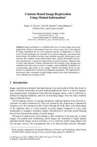
CT Transaxial Chest Image

PET Transaxial Chest Image

Figure 2.1: Transaxial chest images from an anatomical modality (CT) (left), and a functional modality (PET) (right). Images courtesy of Dr. Rob Barnett, Medical Physics Department, Grand River Regional Cancer Center.

the imaging process will produce different images. For example, consider two contrasts: proton density weighted MRI (PD-MRI) and T2 relaxation time weighted MRI (T2-MRI). A proton density sequence used in MR imaging detects the proton density of the object to create a PD-MR image. In comparison, a T2 relaxation time sequence used in MR imaging detects the transverse relaxation time of a proton in its environment to create a T2-MR image [13]. As can be seen in Figure 2.2, the PD-MR image displays dense tissues quite well, but shows little detail in the brain tissue. The T2-MR image, on the other hand, displays brain tissue details quite well. Imaging an object with multiple modalities provides different yet complementary information about the object. Therefore, combining imaging information from several modalities creates a collection of information from which, for example, improved diagnoses and treatments may hopefully be determined. Alternatively, time series information can be collected by using the same imaging modality at multiple times, with time scales ranging from minutes to years. Combining time series imaging information from the same modality creates a collection of information from which, for example, growth 9

PD−weighted MR image

T2−weighted MR image

Figure 2.2: Transaxial brain images from proton density weighted MRI (PD-MRI) (left), and T2 relaxation time weighted MRI (T2-MRI) (right). The images are from the National Library of Medicine’s Visible Human Project via Dr. Jeff Orchard, School of Computer Science, University of Waterloo.

rates may be determined. When either multiple modality (multimodal) or single modality (monomodal) imaging is performed, the result is a collection of images (or data volumes) that contain corresponding complementary information. For example, in cancer treatment strategies, it is common to use multiple modalities to determine diagnoses and treatment plans. This is because different modalities detect and display the extent and position of cancerous lesions differently. For radiation therapy, CT and MR or CT and PET image data are often obtained of the cancerous region. CT data is used to initially locate the target region and to plan the radiation treatment dosages. MR or PET data is used to improve the target region definition. Combining multimodal image information allows diagnosticians to better determine the affected areas, and thus the best treatment plans. It is not guaranteed that the images to be combined have the same resolution or contain the same field of view of the object. Also, the object may appear to be deformed, for example, twisted or enlarged, from one image

10

to the other. Therefore, in order to easily interpret the corresponding information contained in two images, the image space of one image must be aligned to the image space of the other. This process is called registration. Image registration involves finding a transformation of one image space onto the other which best aligns the common features contained in both images. Once the images are registered, the corresponding features of the images are more easily related [15]. Registration of images from the same modality is called intramodal registration and registration of images from different modalities is called intermodal registration.

2.2

Image Registration

We now formally pose the image registration problem. Suppose there are two images, A and B, to be registered. The aim of image registration is to find the transformation, T, which best aligns the position of features in image B, the study image, to the position of the corresponding features in image A, the target image. An image may be considered a mapping of points in the field of view, or domain, Ω, to intensity values [15], that is, A : xA ∈ ΩA → A(xA ) B : xB ∈ ΩB → B(xB ).

(2.1)

Since medical images typically have different fields of view, ΩA and ΩB are different. For an object O, imaged by both A and B, a position x ∈ O is mapped to xA by image A and to xB by image B. Registration finds the spatial transformation, T, which maps xB to xA over the region of overlap, or the intersection of the target image space with the transformed study image space. More specifically, T maps from ΩB to ΩA within the region of overlap

11

ΩT A,B [15], defined as: −1 ΩT A,B = {xA ∈ ΩA : T (xA ) ∈ ΩB }.

(2.2)

This notation emphasizes the dependence of the region of overlap on the original images A and B, as well as the transformation T.

2.2.1

Classification and Validation

Each image registration problem is different and can be characterized by a long list of classifications. The main classifications include: the dimensionality - the inputs may be two- or three-dimensional images; the transformation type, T, which may be specified as a rigid-body, affine, or nonlinear transformation; and the optimization procedure - most methods involve iteratively determining T while optimizing a cost function. Image registration may be performed on 2D to 2D images, 3D to 3D volumes, and 2D images to 3D volumes. 2D to 3D registration is necessary when the 2D image is projective. For example, x-rays are projective since 3D information is projected onto a 2D film. Rigid-body transformations involve the translation and rotation of one image with respect to the other. Affine transformations add scalings and skews to rigid-body transformations. Nonlinear transformations typically follow laws of dynamics described by thin-plate, elastic, or fluid motions, for example. Generally, nonlinear transformations must be regularized to ensure object geometry is not destroyed. For most registration methods, a cost function is optimized using an optimization strategy, such as gradient descent, and iteratively determining the transformation. To evaluate the cost function at each step, the current transformation, T, is applied to image B to adjust the alignment and resample the image into the image space of image A. Transforming the image involves 12

interpolating between data points of image B to determine the transformed image, B T , which lies in ΩT A,B . The interpolation method used to transform the image will affect the registration result since interpolation introduces errors and tends to blur data [15]. The cost function, in general, is a function of A and B T over ΩT A,B . A major problem with some optimization strategies is that the transformation may converge to an incorrect solution, or local optimum of the cost function, instead of the desired solution [15]. As we show in Chapter 4, however, there is no guarantee that the desired solution lies at the global optimum. Image registration problems tend to have many degrees of freedom, thus the parameter space of the optimization method is quite large. As a result, the time required for convergence may also be quite large. Multiresolution approaches [32] have been successfully used to speed up the optimization process and avoid unwanted local optima. Two stage registration methods have also been used to this effect [29]. The best way to ensure correct and quick convergence, however, is to start the optimization strategy with a good initial guess for the transformation. In clinical settings, image registration should ideally be performed in real-time. This demand requires registration algorithms to be computationally efficient, stable, and robust. A major concern with new registration algorithms is validation, i.e., how fast and stable is the algorithm and how accurate is the resulting registration. Existing validation techniques include visual inspection of the registration result, comparison with a gold standard, and evaluation of quantitative measures [15]. Visual inspection evaluation studies involve surveying multiple diagnosticians to rate registration results. The most straight forward validation technique is comparison to a gold standard. A gold standard is a registration technique with proven stability and accuracy. The performance of a new registration algorithm is measured against the existing standard in categories such as the number of successful alignments and the quality of each 13

alignment. Quantitative measures often use statistical analyses of anatomical landmark differences to determine registration accuracy [35]. In [9], the discrete wavelet transform is applied to the problem of quantitatively comparing various registration algorithms. In this thesis, we use visual inspection, the L2 norm, and mutual information to measure the accuracy of registration results. The L2 norm assumes a constant relationship exists between corresponding image intensity values, therefore, registered images with differing intensity maps may not necessarily result in good accuracy ratings, see Section 2.3.1 for more details. The use of mutual information to measure accuracy avoids the issue of dependence on intensity maps, however, mutual information is affected by limited samples contained in the region of overlap. This problem will be discussed more thoroughly in Chapter 4 and Chapter 5.

2.2.2

Landmark- and Surface-Based Registration

For landmark-based registration, a diagnostician is required to manually define landmarks, or points of reference, in one image, and the corresponding points in the other image. Landmark points may be internal, such as bifurcation points of vessels [21] or bones, or external, such as fiducial markers placed on the skin or immobilization frame used in the imaging process. Fiducial markers are small, inert bead-like objects placed in bone, on skin, or on the frame, which have special properties to make them visible in the resulting image. The registration transformation is formed by extrapolating the transformation that aligns the sets of corresponding points. Landmark-based registration has evolved from simple, non-iterative, rigid-body transformation methods to complex, iterative, nonlinear transformation methods. Most nonlinear registrations use landmarks to define the initial and final positions of the transformation and modelled dynamics to govern the deformations. 14

Large deformations typically require the use of fluid dynamics [3], [4], while small deformations can use linear elasticity [5], thin-plate splines [2], etc.. A simple non-iterative, rigid-body transformation, landmark-based registration algorithm involves computing the average or centroid of each set of points (each set containing at least three points) [15]. The distance between the centroids gives the translation required for the registration transformation. The point set is then rotated about the translated centroid until the cost function is minimized. A common cost function for landmark registration is the discrete L2 norm, see Formula A.2 in Appendix A, or sum of squared distances (SSD), Equation (2.5) below, between corresponding point pairs. The root mean square error (RM SE), Formula A.3 in Appendix A, of corresponding points provides a quantitative measure of the registration result and is a common feature in many commercial registration packages [15]. RM SE does not, however, give any indication of the accuracy of alignment between corresponding features. In fact, it may be misleading since a change in landmark location which reduces RM SE may actually increase alignment errors between corresponding features. Including more points in the landmark sets is one way of reducing landmark location identification errors [15]. Landmark-based registration algorithms, by design, use a limited amount of information from the images in order to determine the transformation. Because fiducial markers are reliable and easy to identify, fiducial landmarkbased image registration has long been considered the gold standard of image registration [17]. Similar to landmark-based registration, curve- or surface-based registration determines the transformation which minimizes a cost function that is typically a measure of distance between two corresponding curves or surfaces [15]. In medical images, boundaries are usually more distinct than individual points, and segmentation tools can be used to automatically detect and extract significant curves or surfaces from the images. Auto-segmentation

15

mostly eliminates the necessity of user interaction, although manual editing or adjusting may be required. Most surface-based registration techniques are based on the iterative closest point algorithm [15]. In medical image registration, the iterative closest point algorithm typically represents one surface as a set of points and the corresponding surface as a set of triangular patches. The algorithm has two steps and then iterates until a threshold is reached. The first step identifies the closest point in the set of triangular patches to each of the points on the surface. The closest point is found by linearly interpolating across the facets of each triangle. The second step is to find the least square rigid-body transformation for these point sets (a landmark-based registration). The algorithm then redetermines the closest point set and continues until the minimum distance threshold is achieved. Nonlinear transformations have been implemented into surface-based registration algorithms but generally require good initial conditions in order to converge properly [23]. Surface-based registration uses more image information than landmark-based registration. Unfortunately, it is highly dependent on the segmentation process and user interaction may be required to manually adjust segmentation results. One problem with surface-based registration is that surfaces that have natural symmetries with respect to certain rotations can result in multiple solutions. One possible way to resolve this problem is to perform the surface-based registration several times with various initial rotation estimates. The best alignment of the resulting transformations is then chosen as the final solution.

2.3

Similarity Measures

A different approach to image registration is that of pixel (or voxel) similarity measures. These methods are not based on segmented or delineated features 16

contained in the images, but rather on the intensities of the pixels or voxels contained in the region of overlap of the images. Thus, no user interaction is required and image information is not reduced to a sparse set for registration. The registration transformation is found by optimizing a similarity measure computed from the pixel intensity values of both images over the region of overlap. Therefore, a large portion of the information in each image is used in the alignment process. This tends to average out noise and other errors that may be present in images [15]. Pixel- and voxel-based methods are slowly replacing frame and invasive fiducial landmark-based methods as the gold standard for registration accuracy [23]. Sub-pixel and sub-voxel accuracy is often attainable by similarity measure optimizing registration algorithms [24]. Such algorithms are typically robust, meaning small variations in initial conditions result in small variations in resulting registration transformations. The main disadvantages to registration using similarity measures are the high computational cost associated with optimization algorithms and the inherent limitations associated with subject general similarity [1]. The demand for accuracy and the increasing power of computers, however, makes similarity measure optimizing registration algorithms clinically feasible.

2.3.1

Intramodal Similarity Measures

The similarity measure chosen for a particular registration problem will depend on the type of images involved. If the images are of the same modality, then measures that look for linear or constant relationships between intensity values of corresponding pixel pairs are typically used. Such measures tend to be the simplest measures used for registration. Examples include the correlation coefficient (2.3) and the sum of squared differences (2.5). The correlation coefficient (CC), a normalized version of the cross correlation measure (Formula A.4 in Appendix A), involves the product of the 17

difference from the image mean of corresponding intensity values [22]: − A)(B T (xA ) − B T ) CC =   21 , P P 2 T T 2 xA (B (xA ) − B ) xA (A(xA ) − A) P

xA (A(xA )

(2.3)

where the summations occur over xA ∈ ΩT A,B , A is the mean of image A T is the mean of the transformed image B T over ΩT . over ΩT A,B , and B A,B To register images, the correlation coefficient is maximized. The maximum value corresponds to the strongest linear relationship between corresponding pairs of intensity values [15]. We can consider the correlation coefficient to be the cosine of the angle between the zero-mean vectors (A − A) and (B T − B T ). The maximum value of the cosine of the angle occurs when the angle is minimized, thus implying that the two vectors are as close to being linearly related as possible. Intramodal registration is most commonly used for time series analysis in order to detect subtle changes or contrast enhancements. For images of the same modality, a subtraction image can be formed after registration by subtracting the registered study image from the target image. If the subtraction image shows only noise with no structure, then no changes have occurred. If the subtraction image shows structure, then either small changes have occurred in the object over the imaging period, or, the images were misregistered. Subtraction images can only be used when the images are of the same modality; this ensures that the intensity maps of the images are consistent. If the intensity maps are different, the subtraction image would show structure everywhere, even if no changes in the object had occurred. To register images for subtraction purposes, it is common to use measures based on the discrete L1 and L2 norms, Formula A.1 and Formula A.2 respectively, in Appendix A. In the image registration literature, measures based on these norms are the sum of absolute differences (SAD) and the sum of squared differences (SSD), respectively. Let N be the number of pixels in 18

ΩT A,B , then, SAD = and SSD =

1 N

1 N

X

|A(xA ) − B T (xA )|,

(2.4)


2 A(xA ) − B T (xA ) .

(2.5)

xA ∈ΩT A,B

X xA ∈ΩT A,B

These measures are normalized to be invariant of the number of pixels in the overlap region ΩT A,B . The registration transformation is found by minimizing the measure, i.e., minimizing the structures visible in the subtraction image. It was shown in [36] that the L2 norm is the optimal similarity measure for registering images that differ by Gaussian noise, see Formula A.5 in Appendix A. Since the noise present in medical images is not, in general, Gaussian, the L2 norm is not guaranteed to be the optimal measure for registration. The L2 norm is a satisfactory similarity measure for images with the same intensity maps (i.e., images from the same modality and contrast), and it is commonly used because of its relatively easy implementation. Since the L2 norm is highly sensitive to outliers, the L1 norm is often used to reduce the effect of these large intensity differences [15]. In summary, the correlation coefficient assumes that a linear relationship exists between corresponding pixel intensity values in the images, while the L2 norm assumes the images differ only by Gaussian noise [26]. These assumptions are not always valid: In particular, for intermodal registration these assumptions fail. Intermodal registration demands more complex similarity measures to account for the vastly different intensity maps the imaging modalities create.

19

2.3.2

Intermodal Similarity Measures

Intermodal images display complementary and shared information about the object in images with different intensity maps. For example, what appears as white in one image may appear as dark grey in the other image, or not appear at all. Therefore, similarity measures used for intermodal registration must be insensitive to differing intensity maps. A simple idea for registering CT and MR images, as suggested by Van den Elsen [34], is to transform the CT intensity map into a map that resembles the MR intensity map. For example, soft tissue which appears dark in CT may be remapped to bright intensity values, and bone which appears bright in CT may be remapped to dark intensity values. Once the two image intensity maps are similar, intramodal similarity measures, such as correlation coefficient, can be used to perform the registration. Partitioned intensity uniformity (P IU ), proposed by Woods [40] for MR and PET image registration, was the first similarity measure for intermodal registration that achieved mainstream use [15]. It is based on the idea that all pixels in image A with a particular intensity value represent the same tissue type, thus, the corresponding pixels in image B should also share a particular intensity value [15]. This assumption holds fairly well for the registration of MR and PET images, but requires the scalp to be removed from the MR images. The assumption does not hold for other intermodal registrations, however, the success of P IU as a similarity measure for MR and PET images created great interest and research in intermodal similarity measures [15]. In 1994, a breakthrough in intermodal similarity measures occurred when Hill et al. [16] proposed the use of the 2D frequency of occurrence histogram to measure image alignment. The 2D histogram, when normalized, is an estimate of the joint probability distribution of intensity values between two images over the region of overlap. The joint probability distribution, r(i, j), 20

of a pair of intensity values, (i, j), gives the probability that intensity value j will occur at a point in image B, when intensity value i occurs at the corresponding point in image A. As the alignment of the images changes, the joint probability distribution changes, becoming more disordered as the images move out of alignment. One way of measuring the disorder of the joint probability distribution is to use information theoretic quantities, specifically, Shannon’s entropy function [28]. A simple information theoretic similarity measure, proposed by Studholme et al. [30] and Collignon et al. [6], is the joint entropy function. Registration is performed by minimizing the joint entropy between the images. If we think of entropy as a measure of information, then the registration problem becomes a minimization problem, that is, we attempt to minimize the information present in the overlayed images, see Figure 2.3. Unfortunately, joint entropy is not robust, since often misalignments result in lower joint entropy values than the desired alignment.

+

=

Figure 2.3: Two images to be registered displaying complementary and shared information. At registration, the overlayed images contains less information (two eyes) than the unregistered images (four eyes).

Mutual information, also borrowed from information theory, was proposed as a similarity measure independently by Collignon et al. [6] in 1995 and Wells et al. [39] in 1996. Mutual information is the difference between the information contained in each image over the region of overlap (the entropies) and the information contained in the overlayed images over the region of overlap (the joint entropy). Image registration is performed by maximizing mutual information. This involves maximizing the information contained in each image while minimizing the information contained in the overlayed 21

images. Normalized mutual information, proposed by Studholme et al. [31], is a robust similarity measure that allows for fully automated intermodal image registration algorithms. Similarity measures borrowed from information theory are applicable to both intramodal and intermodal registration problems. The algorithms are usually fully automated and make no assumptions about the relationship between image intensity maps. Registration problems using joint entropy or mutual information become optimization problems, and are computationally expensive since there are no analytic optimizers for these measures [26]. The next chapter provides a more detailed discussion of information theory and some of these similarity measures. Many similarity measures have been proposed for image registration. A good list can be found in [23]. Some methods of interest not discussed above employ tools such as the Fourier transform, optical flow theory, and Taylor expansions. In general, normalized mutual information is used with rigidbody and affine transformation registration problems, whereas landmarks or surfaces are used with nonlinear transformation registration problems.

2.4

Image Fusion

Once image registration has been performed, the problem of how to meaningfully display the registered images remains. This problem is called image fusion. Simple visualization techniques generally used in commercial software packages include: cutaways, checkerboards, outline overlays, and colour overlays [15]. These methods do not combine image information, but rather display information from either one image or the other. Cutaways display half the image information from one image, and the other half of the information from the other image. The dividing line can generally be interactively adjusted to alter the ratio of the displayed image information. 22

Checkerboards use a similar technique but alternate the image information in a checkerboard pattern. Outline overlays display the outline of a structure from one image over top of the other image, while colour overlays display one image in one colour, say red, with the other image placed over top in a different colour, say blue. Other visualization techniques attempt to use mathematical tools to construct one combined, or fused, image. Such techniques may involve operators such as add, subtract, average, or maximum of corresponding intensity values [7], or transformations such as the wavelet transform [38]. The main problem with attempting to combine medical images in these ways is that the image information used by diagnosticians to determine diagnoses and treatments may be lost in the fusion process. For instance, a CT image represents attenuation coefficients of radiation while a PD-MR image represents proton density. If these two images are combined, for example, by choosing the maximum intensity value for each corresponding pixel pair, the meaning of the pixel intensity value in the fused image is lost, i.e., the fused image no longer represents attenuation coefficients or proton density. Nevertheless, image fusion is a useful tool for medical image analysis. Unfortunately, it is highly dependent on registration since misaligned images create poor fused images. To simplify registration problems, modalities such as CT and PET are being combined into one imaging device to reduce the occurrence of deformations, and thus facilitate image registration and fusion [33].

23

Chapter 3 Basics of Information Theory Information theory attempts to characterize the information of random variables. It was developed out of Shannon’s pioneering work in the 1940’s at Bell Laboratories [28]. His work focused on characterizing information for communication systems by finding ways of measuring data based on the uncertainty or randomness present in the given system. Shannon proved that for probabilities pi , X pi log pi − i

is the only functional form that satisfies all the conditions that a measure of uncertainty should satisfy. For a discussion of these conditions see [15, page 57]. Shannon named this quantity entropy because it shares the same mathematical form as the entropy of statistical mechanics. Entropy is one of the main building blocks of information theory. From it, are obtained two other major building blocks, relative entropy and mutual information (MI). These quantities are functionals of probability distribution functions for random variables. Entropy is a measure of uncertainty (or information) in a random variable; relative entropy is a distance measure between one probability distribution and another; and mutual information

25

is the amount of information that one random variable contains about another [8]. We present these information theoretic quantities in relation to mathematical imaging and discuss some of their useful properties. Examples are also presented to demonstrate the behaviour of these quantities.

3.1

Entropy and Information

In mathematical imaging, an intensity image X is represented as a matrix of intensity values. For an n bits/pixel image, the intensity values are the discrete greyscale values X = {x1 , x2 , . . . , xN }, where N = 2n and xk = k−1. A histogram can be constructed from an image by looking at each pixel intensity value and counting the number of times a pixel intensity value occurs, or the number of times a pixel intensity value lies in a range, or bin, of intensity values. Dividing the histogram of occurrences by the total number of pixels in the image gives the frequency of occurrence of each intensity value, or each intensity value bin. Normalizing the histogram in this way gives an estimate of the probability distribution function of pixel intensity values for the image. Given an image X, we use p to denote the corresponding estimated intensity value probability distribution function, where p(x) = Pr(Xi,j = x), for x ∈ X and Xi,j a pixel in image X. A result of the histogram normalization P is that x p(x) = 1. In statistical literature, this function p is commonly referred to as the probability density function, or the probability mass function. Here we follow the notation used in [8], [15], and [27] and refer to p as the probability distribution function, or simply, the distribution. In order to apply information theory to imaging applications, we must consider an image as a collection of independent observations of a random variable. A random variable is a mapping that assigns a number to each element of a sample space [27]. 26

Definition 3.1.1. Let S be a sample space with elements {ωi }. Then the random variable X is a mapping X:S→R where R is the real number line, i.e., for ωi ∈ S and r ∈ R X(ωi ) = r. Note that X represents both the image and the random variable that determines the image. For images, the random variable X is simply the identity mapping, that is, X(xi ) = xi for xi ∈ X . Furthermore, since the sample space X contains only discrete quantities, the random variable X is discrete. An image is therefore an array of the elements x ∈ X as determined by independent observations of the discrete random variable X. For example, an 8 bits/pixel image has 28 = 256 elements in the sample space of the random variable X, i.e., X = {0, 1, . . . , 255}. The value of X at each of these elements is equal to the value of the element, so that X(0) = 0, X(1) = 1, . . . , and X(255) = 255. An M × M pixel image is thus M 2 independent observations of the discrete random variable X organized into a square matrix. From this matrix, the frequency of occurrence method can be used to estimate the probability distribution of the random variable. Example 3.1.2. Consider the 8 bits/pixel image shown on the left of Figure 3.1. Starting from the upper left hand corner, the associated histogram is constructed by traversing through each row and column counting the number of times a pixel intensity value occurs. The associated histogram is shown in the middle of Figure 3.1. Dividing each count by the total number of pixels contained in the image creates an estimate of the probability distribution of the image. The estimated probability distribution is shown on the right of Figure 3.1.

27

Image Histogram

Image Distribution 0.08

Image

0.06

1000

0.04 500 0.02 0 0

100

200

0

0

100

200

Figure 3.1: An image of the author (left) and the associated histogram (middle) and probability distribution estimate (right).

Entropy uses probability distribution functions to measure the randomness or uncertainty of a random variable. Under the assumption that each observation in the image matrix is independent and occurs with the probability determined by the frequency of occurrence, the entropy of the random variable X, or the entropy of the image, can be computed [27]. Definition 3.1.3. The entropy, H(X), for the discrete random variable X, with probability distribution function p, is defined as H(X) = H(p) = −

X

p(x) log p(x),

x∈X

where, for reasons of continuity, we define 0 log 0 = 0. Note the entropy of X, H(X), may also be denoted H(p). The notation H(p) emphasizes the dependence of entropy on the probability distribution of X, as opposed to the actual intensity values of X. For example, an image that is half black and half white has the same entropy as an image that is half black and half grey. The notation H(X) is ambiguous so that X can be interpreted as either the image or the discrete random variable that determines the image. 28

In Definition 3.1.3, log is taken to mean log2 so that entropy is measured in bits (binary digits). Changing the base of the logarithm will rescale the entropy and change the measurement units. A logarithm with base e is measured in nats, while a logarithm with base 10 is measured in hartleys. In this work, we assume the base to be 2 so that entropy represents the amount of binary information required on average to describe the random variable [8]. Example 3.1.4. Returning to Example 3.1.2, the entropy of the probability distribution estimate shown on the right of Figure 3.1, computed using Definition 3.1.3, is 6.71 bits.

3.2

Joint Entropy and Mutual Information

We now move on to consider information measures for multiple images. Following the ideas outlined above, we consider two images (over their region of overlap) to be observations of two discrete random variables, X and Y , with probability distributions p and q respectively. In general, random variable X will have sample space X and random variable Y will have sample space Y . For imaging purposes, the modality-specific intensity maps determine X and Y . The 2D joint histogram can be constructed from images X and Y over their region of overlap by counting the number of times the intensity pair (x, y) occurs in corresponding pixel pairs (Xi,j , Yi,j ). Normalizing the joint histogram gives an estimate of the joint probability distribution r, where r(x, y) = P r(Xi,j = x, Yi,j = y), for x ∈ X , y ∈ Y and (Xi,j , Yi,j ) corresponding pixels contained in the region of overlap. A result of the joint P P histogram normalization is that x y r(x, y) = 1. The image distributions are related to the joint distribution by (3.1), and in this respect are termed

29

the marginals of the joint distribution: X

r(x, y) = q(y)

and

x∈X

X

r(x, y) = p(x).

(3.1)

y∈Y

Joint entropy, H(X, Y ), is a functional of the joint probability distribution r, and is a measure of the combined randomness of the discrete random variables X and Y . It is a simple extension of entropy since the pair of random variables (X, Y ) may be considered a single vector-valued random variable [8]. Definition 3.2.1. The joint entropy, H(X, Y ), for the discrete random variables X and Y , with joint probability distribution r, is defined as XX

H(X, Y ) = H(r) = −

r(x, y) log r(x, y).

x∈X y∈Y

If two random variables are independent, then the joint probability distribution becomes the product distribution d, that is, r(x, y) = d(x, y) = p(x)q(y). In this situation, joint entropy simplifies to: H(X, Y ) = −

X

=−

X

r(x, y) log r(x, y)

x,y

p(x)q(y) log p(x) −

x,y

X

p(x)q(y) log q(y)

x,y

= H(X) + H(Y ). In general H(X, Y ) ≤ H(X) + H(Y ), with equality if and only if X and Y are independent. This result follows from Corollary 3.3.4, to be presented below. Relative entropy, or Kullback-Leibler distance, is a measure of the distance between one probability distribution and another. It measures the error of using an estimated distribution q over the true distribution p [8]. 30

Definition 3.2.2. The relative entropy, D(p k q), of two probability distributions p and q over X , is defined as D(p k q) =

X x∈X

p(x) log

p(x) , q(x)

where, for reasons of continuity, we define 0 log 0q = 0 and p log p0 = ∞. A special case of relative entropy is mutual information. Mutual information measures the amount of information shared between two random variables, or the decrease in randomness of one random variable due to the knowledge of another [8]. Definition 3.2.3. Let X and Y be two random variables with probability distributions p and q, respectively, and joint probability distribution r. Mutual information, I(X; Y ), is the relative entropy between the joint probability distribution, r, and the product distribution, d, where d(x, y) = p(x)q(y). That is, I(X; Y ) = D(r k d) XX r(x, y) = . r(x, y) log p(x)q(y) x∈X y∈Y Recall that if the random variables X and Y are independent, then the joint probability distribution is equal to the product distribution, i.e., r = d. Thus, mutual information measures the correlation between X and Y , with respect to X and Y being independent. Using (3.1) in Definition 3.2.3 allows mutual information to be expressed in terms of entropy: I(X; Y ) = H(X) + H(Y ) − H(X, Y ).

(3.2)

This relationship is expressed by the Venn diagram [8] shown in Figure 3.2. 31

H(X,Y)

I(X;Y)

H(X)

H(Y)

Figure 3.2: The relationship between entropy, joint entropy, and mutual information.

3.3

Properties of Information

In order to gain a better understanding of entropy, relative entropy, and mutual information, some properties and simple examples are presented below. Non-negativity is an important property of information measures since negative information is not physically meaningful. Lemma 3.3.1. Entropy is a non-negative quantity, i.e., H(p) ≥ 0. Proof. Since p is a normalized probability distribution, 0 ≤ p(x) ≤ 1 for all x ∈ X . Thus, −p(x) log p(x) ≥ 0 so that H(p) ≥ 0. It can also be shown that relative entropy is non-negative. This theorem is the basis of many fundamental results in information theory [11]. Theorem 3.3.2. Let p and q be two probability distributions over X , then D(p k q) ≥ 0 and equality holds if and only if p(x) = q(x) for all x ∈ X . 32

Proof. Let A = {x ∈ X : p(x) > 0} be the support of p. Then −D(p k q) = −

X

p(x) log

x∈X

=

X

p(x) log

x∈A

p(x) q(x)

q(x) p(x)



 q(x) ≤ p(x) −1 p(x) x∈A X X = q(x) − p(x) X

x∈A

≤

X

x∈A

q(x) −

x∈X

X

p(x)

x∈A

= 1 − 1 = 0, where we have used the fact that log t ≤ t − 1 and equality holds if and only q(x) if t = 1, i.e., p(x) = 1 for all x ∈ A, or p = q. Since relative entropy is a measure of distance, it would be convenient if it was a distance metric. Unfortunately, relative entropy is not a metric since it satisfies neither the symmetry property nor the triangle inequality. We demonstrate the failure of symmetry with the following example. Example 3.3.3. Consider two binary random variables X and Y , with sample spaces X = Y = {0, 1} and probability distributions p = (s, 1 − s) and q = (t, 1 − t), respectively, (0 ≤ s, t ≤ 1). The relative entropy between p and q is s 1−s D(p k q) = s log + (1 − s) log , t 1−t while the relative entropy between q and p is D(q k p) = t log

t 1−t + (1 − t) log . s 1−s

It is easy to see that if s = t then D(p k q) = D(q k p) = 0. If s = 0 and 33

t = 12 , however, then D(p k q) = 1 while D(q k p) = ∞. The following corollary is a direct result of Theorem 3.3.2 and states that mutual information is non-negative. Corollary 3.3.4. The mutual information for any two random variables X and Y is non-negative, i.e., I(X; Y ) ≥ 0, with equality if and only if X and Y are independent. Proof. Using Theorem 3.3.2, I(X; Y ) = D(r(x, y) k p(x)q(y)) ≥ 0 with equality if and only if r(x, y) = p(x)q(y), or the random variables are independent. Combining (3.2) and Corollary 3.3.4, we can now relate the entropy of two random variables to their joint entropy. That is, from 0 ≤ I(X; Y ) = H(X) + H(Y ) − H(X, Y ), we get H(X, Y ) ≤ H(X) + H(Y ), with equality if and only if X and Y are independent. Thus, the combined information of two dependent random variables must be less than the sum of the information of each variable on its own. Definition 3.3.5. A concave function f : R → R is a function that satisfies: f (λx1 + (1 − λ)x2 ) ≥ λf (x1 ) + (1 − λ)f (x2 ) for 0 ≤ λ ≤ 1 and for all x1 , x2 in the domain of f . 34

Concavity is also known as concave down or convex down. Examples √ of concave functions include ln x, x, and −x log x, for x ≥ 0. Theorem 3.3.6 states that entropy is a concave function and provides upper and lower bounds on the entropy of a linear combination of probability distributions. Theorem 3.3.6. For two random variables X and Y with sample space X , respective probability distributions p and q, and some parameter c, 0 ≤ c ≤ 1, entropy satisfies cH(p) + (1 − c)H(q) ≤ H(cp + (1 − c)q) ≤ cH(p) + (1 − c)H(q) + h(c), where h(c) is the entropy of a binary random variable with probability distribution (c, 1 − c). The first inequality shows that entropy is a concave function of p [11]. Proof. This proof follows similar reasoning to the proof presented in [11]. First note that cp(x) + (1 − c)q(x) ≥ cp(x), and similarly for q(x). Thus, − log (cp(x) + (1 − c)q(x)) ≤ − log (cp(x)) and − log (cp(x) + (1 − c)q(x)) ≤ − log ((1 − c)q(x)) .

35

To prove the right hand inequality we have, H(cp + (1 − c)q) = −

X

(cp(x) + (1 − c)q(x)) log (cp(x) + (1 − c)q(x))

x∈X

= −c

X

p(x) log (cp(x) + (1 − c)q(x))

x∈X

− (1 − c)

X

q(x) log (cp(x) + (1 − c)q(x))

x∈X

≤ −c

X

p(x) log (cp(x))

x∈X

− (1 − c)

X

q(x) log ((1 − c)q(x))

x∈X

= cH(p) + (1 − c)H(q) + h(c), where h(c) = − c log(c) − (1 − c) log(1 − c). To prove the left hand inequality let A = {x ∈ X : p(x) > 0} be the support of p and let B = {x ∈ X : q(x) > 0} be the support of q. Starting

36

from the second line above, we have that, H(cp + (1 − c)q) = − c

X

p(x) log (cp(x) + (1 − c)q(x))

x∈X

− (1 − c)

X

q(x) log (cp(x) + (1 − c)q(x))

x∈X



 q(x) = −c p(x) log p(x) c + (1 − c) p(x) x∈A    X p(x) − (1 − c) q(x) log q(x) c + (1 − c) q(x) x∈B X



= cH(p) + (1 − c)H(q)   X q(x) −c p(x) log c + (1 − c) p(x) x∈A   X p(x) − (1 − c) q(x) log c + (1 − c) . q(x) x∈B

Using log t ≤ t − 1 for t ≥ 0, we can simplify the last two terms as follows: −c

X x∈A



q(x) p(x) log c + (1 − c) p(x)

 ≥ −c

X x∈A

= −c

X



 q(x) p(x) c + (1 − c) −1 p(x) (cp(x) + (1 − c)q(x) − p(x))

x∈A

≥ − c (c + 1 − c − 1) = 0, where we have used the fact that

P

x∈A

 p(x) − (1 − c) q(x) log c + (1 − c) ≥ 0. q(x) x∈B X



q(x) ≤ 1. Similarly,

37

We will return to the above result later in this thesis. The next theorem provides an upper bound on the entropy of a probability distribution, and gives insight into the nature of this information measure. The theorem shows that the maximal value of entropy occurs when the probability distribution is the uniform distribution. That is, the random variable X is most random, i.e., entropy or information is maximized, when each element of X is equally likely. Theorem 3.3.7. The maximal value of entropy is log N , where N is the number of elements in X . This maximal value occurs when p is the uniform distribution over X , i.e., p = u, where u(x) = N1 for all x ∈ X . Proof. Let p be a probability distribution over X , and let u be the uniform distribution over X , i.e., u(x) = N1 for all x ∈ X , where N is the number of elements in X . From Theorem 3.3.2 we have, 0 ≤ D(p k u) X p(x) = p(x) log u(x) x∈X X X 1 = p(x) log p(x) − p(x) log N x∈X x∈X = −H(p) + log N.

Thus, H(p) ≤ log N with equality if and only if p = u. We conclude this discussion with the following example which demonstrates a few of the properties of entropy using a simple binary random variable.

38

Example 3.3.8. Consider the binary random variable X, such that ( X=

0 with probability p, 1 with probability 1 − p.

Here p = (p, 1 − p), so the entropy of X is H(p) = −p log p − (1 − p) log(1 − p). Differentiating with respect to p and simplifying we get dH(p) 1−p = log . dp p = 0 gives p = 12 , with H(p) = log 2 = 1. The second derivative Solving dH(p) dp with respect to p is −1 d2 H(p) = < 0 ∀p. 2 dp p(1 − p) Thus, by the second derivative test, the entropy of a binary random variable is concave, with a maximum value of 1 at p = 12 . A plot of H(p) as a function of p is shown in Figure 3.3. To relate this example to Theorem 3.3.7, p = (p, 1 − p), X = {0, 1}, and N = 2. As expected, the maximum value of H(p) is log N = log 2 = 1, which occurs when the distribution is uniform, i.e., p = ( 12 , 21 ). Notice that when p = (0, 1) or p = (1, 0), the entropy is zero. Since these two limiting cases correspond to fixed variables, X = 0 or X = 1 always, there is no uncertainty in the random variable, and hence information (entropy) is zero. The above example demonstrates that the entropy of a random variable is maximum when the random variable is most unpredictable, or most uncertain. Thus, the entropy of an image will be maximal when the probability distribution is uniform. In this case, each intensity value will be equally likely 39

Entropy of Binary Random Variable 1

Entropy

0.8 0.6 0.4 0.2 0

0

0.5 p

1

Figure 3.3: The entropy of a binary random variable as a function of p.

to occur in a given pixel of the image. We now move on to apply information theory to the problem of image registration.

40

Chapter 4 Image Registration Using Information Theory This chapter discusses the information theoretic similarity measures, joint entropy and mutual information. We begin with a discussion of probability distribution estimation with specific attention to the region of overlap and then move on to discuss joint entropy and mutual information as similarity measures with examples to highlight their advantages and disadvantages in image registration.

4.1

Distribution Estimation

In this work, image distributions are estimated by normalizing the frequency of occurrence histogram. This simple technique must be computed for every iteration of the registration process and is affected by factors such as, the number of intensity bins used in the histogram, degradations present in the images, and the interpolation method used to transform the images. Therefore, consistency is important among these, and other, factors during

41

distribution estimation. For large scale medical imaging problems, estimating distributions in this fashion is computationally expensive. Thus, it is common to use image distribution estimates based on a sample drawn from the image. Such distribution estimates are usually a mixture of Gaussians, see Formula A.5 in Appendix A, and are found by Parzen window density estimation with Gaussian window functions [36].

4.1.1

Image Distributions

As discussed in the previous chapter, information theoretic similarity measures are functions of probability distributions of images. An important consequence of using similarity measures based on image statistics, instead of image intensity values, is that images that do not look similar may have similar distributions. Fortunately, since joint distributions incorporate spatial dependence, such images are recognized as being dissimilar. Image X

Image Y

Figure 4.1: The half black, half white binary image X (left), and the checkerboard binary image Y (right).

Example 4.1.1. Consider the binary images X and Y shown in Figure 4.1. Both images have the same distribution, that is, p = q = ( 12 , 21 ). The joint 42

distribution, however, which takes into account spatial dependence between images, is: ! r=

1 4 1 4

1 4 1 4

.

(4.1)

Note the image distributions and their joint distribution are uniform, so all entropies are maximized. The entropy of each image is 1 bit, the joint entropy is 2 bits, and the mutual information is 0 bits, indicating that the images are independent. Intensity Binning In the above example, two intensity bins were used in the histograms of the binary images. For intensity images, the number of intensity bins used can affect the distribution estimates, and hence the entropy estimates. To demonstrate the effects of intensity binning on entropy estimation, we use images of a lime obtained by micro-MRI at two different resolutions: a 256 × 256 pixel image (lime 256 ) and a 64 × 64 pixel image (lime 64 ). The lime images are 16 bits/pixel and are shown in Figure 4.2. 256 X 256 Pixel Lime Image

64 X 64 Pixel Lime Image

Figure 4.2: 256 × 256 pixel lime image, lime 256, (left) and 64 × 64 pixel lime image, lime 64, (right). Images courtesy of Dr. Claude Lemaire, Physics Department, University of Waterloo.

43

The maximum number of intensity bins used in a histogram is equal to the total number of intensity levels in the image. For a 16 bits/pixel image, the maximum number of intensity bins is 216 . For image lime 256, which contains 256 × 256 = 216 pixels, using the maximum number of intensity bins results in a sparse distribution estimate, and thus an inaccurate estimate of the distribution and entropy, see Figure 4.3. To avoid sparse distributions, it is common to use 32 to 256 intensity bins [15]. −3

x 10

16

Distribution with 2

Bins

2 1.5 1 0.5 0

0

2 4 Entropy = 9.38

6 4

x 10

Figure 4.3: Image lime 256 distribution and entropy estimate using 216 intensity bins.

The effects of reducing the number of intensity bins on distribution estimation are shown in Figure 4.4. As the number of histogram intensity bins decreases, the entropy of the distribution estimate also decreases. In the limit, when there is only one histogram intensity bin, the entropy is zero. As the number of intensity bins decreases, the histogram count in each bin increases or stays constant, since the range of intensities associated with each bin widens. This causes the distribution to become less sparse and to appear smoother with larger maxima: entropy is lower since the distribution is less uniform. 44

Distribution with 256 Bins

Distribution with 128 Bins

Distribution with 64 Bins

0.2

0.2

0.2

0.15

0.15

0.15

0.1

0.1

0.1

0.05

0.05

0.05

0

0

100 200 Entropy = 4.07

0

0

50 100 Entropy = 3.39

0

0

20 40 Entropy = 2.72

60

Figure 4.4: Image lime 256 distribution and entropy estimates using 256 (left), 128 (middle), and 64 (right) intensity bins.

To achieve accurate distribution, and hence entropy, estimates, the number of intensity bins should be chosen to avoid sparseness. In this work, 256 intensity bins are used unless otherwise stated. For image lime 256, 256 intensity bins allots 256 intensity levels to each bin with 216 pixel intensity values to distribute among the bins. This is sufficient to create a non sparse distribution estimate. Degraded Images Clinical images are degraded by the presence of noise and blur. For example, images are blurred by patient movement during the imaging process: In PET imaging, the acquisition time is typically about 30 minutes, so the entire breathing cycle occurs many times during acquisition which results in averaging of the collected data. Noise, prevalent in all medical images, is largely introduced by the sensors during acquisition. In MRI, the noise present in the foreground image can be modelled as Rician distributed noise [25], see Formula A.6 in Appendix A. If the signal mean is much greater than the noise variance, then Rician distributed noise can be approximately modelled as Gaussian distributed noise [25]. The inherent degradations of clinical images inhibit accurate estimation of distributions, and hence entropies [14]. 45

To demonstrate the effects of noise and blur on image distribution estimation, we use the horse images shown in Figure 4.5. Zero-mean white Gaussian noise of variance 25.5 has been added to the horse image to create the noisy image, and a Gaussian low-pass filter of standard deviation 10 has been applied to the horse image to create the blurred image. The distributions of the three horse images are shown in Figure 4.6. The presence of noise in the horse image causes the distribution to spread, becoming more uniform over the centre intensity bins and piling up slightly (probability about 0.01) in the limiting intensity bins (bins 0 and 255). As a result of the distribution becoming more uniform, the entropy estimate increases. The presence of blur in the horse image, on the other hand, sharpens the peaks and fills in intermediate intensity bins in the distribution, making the peaks more pronounced and the distribution less uniform which results in an entropy estimate decrease. Resolution and Interpolation Image resolution also affects distribution estimation. Intuitively, since higher resolution images more accurately represent the imaged object than lower resolution images, the entropy estimates based on higher resolution images should more accurately estimate the true entropy. During image registration, it may be necessary to increase (or decrease) the resolution of the study image to match the resolution of the target image. Interpolation, used to transform and resample the study image, introduces artifacts and hence perturbs the image and joint distribution estimates. To examine the effects of increasing resolution, we use image lime 64 and three interpolation methods: nearest neighbour, bilinear, and bicubic. In nearest neighbour interpolation, the intensity value of an interpolated pixel is equal to the intensity value of the closest original pixel. The special case of increasing resolution an integer number of times reduces nearest neighbour 46

Horse Image

Noisy Horse Image

Blurred Horse Image

Figure 4.5: The horse image (left), the noisy horse image (middle), and the blurred horse image (right).

47

0.04

Horse Image Distribution

Noisy Horse Image Distribution Blurred Horse Image Distribution 0.04 0.04

0.03

0.03

0.03

0.02

0.02

0.02

0.01

0.01

0.01

0

0

100 200 Entropy = 7.32

0

0

100 200 Entropy = 7.89

0

0

100 200 Entropy = 7.25

Figure 4.6: Distribution estimates for the horse image (left), the noisy horse image (middle), and the blurred horse image (right).

interpolation to pixel replication. For example, to double the resolution of an image, each row and then each column is duplicated [10]. In bilinear interpolation, the intensity value of an interpolated pixel is equal to the value at that point of a bilinear surface (or hyperboloid) fit through the intensity values of the four closest original pixels. Finally, in bicubic interpolation, the intensity value of an interpolated pixel is equal to the value at that point of a bicubic surface fit through the intensity values of the sixteen closest original pixels [19]. The use of more pixel neighbours and the fitting of more complex surfaces gives smoother interpolation results but results in higher computational costs [10]. In Figure 4.7, the resolution of image lime 64 was increased by a factor of 4 to 256 × 256 pixels using the interpolation methods described above. Nearest neighbour interpolation creates pixel block artifacts in the enhanced image, whereas bilinear and bicubic interpolation create enhanced but blurred images. Image lime 64 was increased in resolution to a 128 × 128 pixel image, a 256 × 256 pixel image, and a 512 × 512 pixel image using each of the interpolation methods discussed above. The distributions of these images are shown in Figure 4.8 with the entropy of each distribution estimate included below the plot. Notice that for nearest neighbour interpolation, neither the 48

Nearest Neighbour Interpolation

Bilinear Interpolation

Bicubic Interpolation

Figure 4.7: Image lime 64 enhanced to 256 × 256 resolution using nearest neighbour (left), bilinear (middle), and bicubic (right) interpolation.

49

Nearest Neighbour Interpolation Bilinear Interpolation Bicubic Interpolation

Lime 64

Increased to 128

Increased to 256

Increased to 512

0.1

0.1

0.1

0.1

0.05

0.05

0.05

0.05

0

0

100 200 Entropy = 3.87

0

0

100 200 Entropy = 3.87

0

0

100 200 Entropy = 3.87

0

0.1

0.1

0.1

0.1

0.05

0.05

0.05

0.05

0

0

100 200 Entropy = 3.87

0

0

100 200 Entropy = 3.83

0

0

100 200 Entropy = 3.84

0

0.1

0.1

0.1

0.1

0.05

0.05

0.05

0.05

0

0

100 200 Entropy = 3.87

0

0

100 200 Entropy = 3.87

0

0

100 200 Entropy = 3.89

0

0

100 200 Entropy = 3.87

0

100 200 Entropy = 3.85

0

100 200 Entropy = 3.90

Figure 4.8: Distribution estimates of image lime 64 (column 1 ) and image lime 64 enhanced to 128 × 128 pixels (column 2 ), 256 × 256 pixels (column 3 ), and 512 × 512 pixels (column 4 ), using nearest neighbour (row 1 ), bilinear (row 2 ), and bicubic (row 3 ) interpolation.

50

distribution nor the entropy changes as the resolution is increased. This is because each pixel is duplicated, triplicated, or quadrupled, depending on the level of resolution enhancement, so the frequencies of occurrence remain constant. For bilinear and bicubic interpolation, as resolution is increased, the images are enhanced, but blurred. As a result, the distributions become smeared due to the re-binning of interpolated intensity values, and slightly sharper due to the presence of blur. For image lime 64, the entropy of the bilinear and bicubic interpolated images varies, with entropy being higher for bicubic interpolation.

256 Bins

Lime 256

Decreased to 64

Decreased to 32

0.2

0.2

0.2

0.2

0.15

0.15

0.15

0.15

0.1

0.1

0.1

0.1

0.05

0.05

0.05

0.05

0

64 Bins

Decreased to 128

0

100 200 Entropy = 4.07

0

0

100 200 Entropy = 4.07

0

0

100 200 Entropy = 4.06

0

0.2

0.2

0.2

0.2

0.15

0.15

0.15

0.15

0.1

0.1

0.1

0.1

0.05

0.05

0.05

0.05

0

0

50 Entropy = 2.72

0

0

0

50 Entropy = 2.72

0

50 Entropy = 2.71

0

0

100 200 Entropy = 4.03

0

50 Entropy = 2.72

Figure 4.9: Distribution estimates using 256 intensity bins (top row ) and 64 intensity bins (bottom row ) of the image lime 256 (column 1 ), and image lime 256 decreased to 128×128 pixels (column 2 ), 64 × 64 pixels (column 3 ), and 32 × 32 pixels (column 4 ) using nearest neighbour interpolation.

The top row of Figure 4.9 shows the distribution estimates using 256 intensity bins for image lime 256 decreased in resolution to 128×128, 64×64, and 32 × 32 pixels by nearest neighbour interpolation. The distribution 51

estimates become increasingly sparse as resolution is decreased. For the 32 × 32 pixel image (and possibly the 64 × 64 pixel image), there are too many intensity bins. As a result, the distribution estimates are jagged and unreliable. The bottom row of Figure 4.9 shows the distribution estimates computed using 64 intensity bins. Even with the reduced number of intensity bins, the 32 × 32 pixel image still creates a jagged distribution estimate. Decreasing image resolution causes distribution estimates to become increasingly jagged due to the diminishing number of pixels, and hence pixel intensity values, to count in the histograms. In general, the entropies of the decreased resolution images are lower than the entropy of the original image because the distributions have become jagged and less uniform. This effect is accentuated by the fact that half of the intensity value range is unused by the lime images. Selective Intensity Binning A better way to estimate the distributions of the lime images from Figure 4.2 is to use selectively spaced intensity bins instead of equally spaced intensity bins, as done above. Since the lime images are encoded at 16 bits/pixel, but only use 215 intensity values, half of the intensity bins in the distribution estimates are empty. Note in Figure 4.9 that the distributions extend over the first half of the intensity bins (x-axis), but are zero for the remaining half. Selective intensity bin spacing can stretch distributions to use all available bins and can group related intensity values into custom bins. Figure 4.10 shows the distributions for image lime 256 decreased in resolution to 128 × 128, 64 × 64, and 32 × 32 pixels using 256 selectively spaced intensity bins. Starting from intensity level 0, each bin contains 128 intensity values while the last bin contains the remaining 32896 intensity values. The effect of these selectively spaced intensity bins is that the distributions are spread across the 52

256 Bins

Lime 256

Decreased to 128

Decreased to 64

Decreased to 32

0.03

0.03

0.03

0.03

0.025

0.025

0.025

0.025

0.02

0.02

0.02

0.02

0.015

0.015

0.015

0.015

0.01

0.01

0.01

0.01

0.005

0.005

0.005

0.005

0

0

0

0

100 200 Entropy = 4.77

0

100 200 Entropy = 4.81

0

100 200 Entropy = 4.79

0

0

100 200 Entropy = 4.78

Figure 4.10: Distribution estimates using 256 selectively spaced intensity bins of image lime 256 (column 1 ) and image lime 256 decreased to 128 × 128 pixels (column 2 ), 64 × 64 pixels (column 3 ), and 32 × 32 pixels (column 4 ) using nearest neighbour interpolation.

entire bin range. The increasing jaggedness of the distributions as resolution decreases is now more pronounced. Note that the entropies of the decreased resolution images are now slightly higher than the original lime 256 image in contrast to the results shown in Figure 4.9. This is because the distributions are more uniform since they extend over the entire bin range. In medical imaging, it might be advantageous to use selective intensity binning when computing distributions. For instance, intensity bin spacing can be customized to group ranges of intensity values that correspond to certain tissue types. The range and spacing of intensity bins can be different for the target and study images to account for the different intensity maps of multimodal images. Selective intensity binning may facilitate image registration by enhancing the correlation of aligned tissues. An alternate way to deal with differing intensity bin ranges is to normalize the images prior to registration. Normalizing an image involves transforming the intensity map to use the standard range of intensity values, i.e., {0, 1, . . . , 255}. Normalizing any image that is encoded higher than 8 bits/pixel into this standard range, however, will result in the loss of information. In applications where image information is vital, such as medical imaging, normalization should be avoided. 53

In medical imaging, any image processing done prior to registration that unnecessarily modifies the image distributions should be avoided. For example, histogram equalization attempts to make image histograms more uniform by remapping intensity values from frequently used intensity bins into less frequently used intensity bins. If successful, histogram equalization causes image entropy to increase, but at the same time, destroys the image information diagnosticians rely on. An imaging modality relates specific anatomical or function details to specific intensity values: By altering the intensity map via histogram equalization, the image will be rendered meaningless.

4.1.2

Joint Distributions

Joint distributions are a way of measuring the spatial correlation between images. In image registration, the region of overlap, or intersection, of the images determines which pixel pairs are used in the joint distribution estimate and hence the marginal distribution estimates. In this section, we assume our images to be registered so that the region of overlap is the entire image space. We return to the PD-MR and T2-MR images shown in Figure 2.2. The images are 8 bits/pixel and have been padded with zeros on the left and right sides to make them 256 × 256 pixel arrays. Recall that these images are from the same modality (MRI), but, because they were obtained using different pulse sequences, their intensity maps are different. In PD-MRI all hydrogen atoms in the object contribute to the image; in T2-MRI only a select set of the hydrogen atoms contribute to the image [1]. Thus information contained in PD-MR and T2-MR images is highly correlated. The distributions of the MR images and of the MR images with most of the background and zero padding cropped out are shown in Figure 4.11. The top row shows the distributions for the uncropped images: Note the large spike around zero caused by the image padding. The bottom row shows 54

the distributions for the cropped images. Cropping images by removing unnecessary background increases the nonzero probability values of the distribution estimates to focus the distribution on the foreground object. This ensures registration of the foreground object instead of registration of the background. Cropping images results in increased entropy estimates because the removal of the large spike at zero causes distributions to become more uniform. The following work uses the cropped MR images (235 × 180 pixels) unless otherwise stated. PD−MR image distribution

T2−MR image distribution

0.25

0.25

0.2

0.2

0.15

0.15

0.1

0.1

0.05

0.05

0

0

50

100 150 Entropy = 6.09

200

0

250

0

Cropped PD−MR image distribution 0.035

0.03

0.03

0.025

0.025

0.02

0.02

0.015

0.015

0.01

0.01

0.005

0.005 0

50

100 150 Entropy = 7.41

200

100 150 Entropy = 5.80

200

250

Cropped T2−MR image distribution

0.035

0

50

0

250

0

50

100 150 Entropy = 7.13

200

250

Figure 4.11: Image distribution and entropy estimates for the uncropped PD-MR (top left) and T2-MR (top right) images and for the cropped PD-MR (bottom left) and T2-MR (bottom right) images.

In the PD-MR image distribution, the leftmost hill, comprised of intensity values 0 to 35, represents the noisy background surrounding the head; the plateau, intensity values 35 to 150, represents the skull and tissues surrounding the brain and eyes; and the rightmost hill, intensity values 150 to 55

255, represents the brain tissue and eyes. In the T2-MR image distribution, the leftmost hill, intensity values 0 to 40, represents the noisy background and the tissues surrounding the brain, eyes and sinus cavity; the plateau, intensity values 40 to 80, represents tissue details in the regions surrounding the brain and eyes; the middle hill, intensity values 80 to 175, represents the brain tissue; and the rightmost hill, intensity values 175 to 255, represents the eyes. Recall that for two images X and Y , each pixel pair (Xi,j , Yi,j ) has an associated intensity pair (x, y), where x ∈ X is the intensity value at pixel Xi,j in X, y ∈ Y is the intensity value at the corresponding pixel Yi,j in Y , and (i, j) are the indices for the image matrices over the region of overlap. The joint distribution represents the probability of intensity pair (x, y) occurring at corresponding pixels in X and Y . To enhance the printable display of joint distributions, zero probability is coloured black (0), probability values greater than the threshold T = 4.0 × 10−5 are coloured white (255), and probability values in between these limits are linearly interpolated shades of grey. Joint Distribution for Cropped PD−MR image

Product Distribution for Cropped PD−MR image

250

250

200

200

150

150

100

100

50

50

50

100 150 200 Joint Entropy = 7.41

250

50 100 150 200 Joint Entropy = 14.82

250

Figure 4.12: Joint distribution (left) and product distribution (right) estimates for the PD-MR image with itself at registration.

The joint distribution of an image with itself at registration demonstrates 56

perfect correlation. In Figure 4.12, the joint distribution of the PD-MR image with itself at registration is shown on the left and the product distribution is shown on the right. The joint distribution is only nonzero along the line y = x, indicating that if intensity value x occurs in pixel Xi,j , then it must also occur in pixel Yi,j . Recall that product distributions occur when two images are independent. Mutual information is a measure of the distance from the joint distribution to the product distribution. For this example, mutual information is maximized since the images are correctly aligned. Joint Distribution for Cropped MR images

Product Distribution for Cropped MR images

250

250

200

200

150

150

100

100

50

50

50 100 150 200 Joint Entropy = 12.78

250

50 100 150 200 Joint Entropy = 14.54

250

Figure 4.13: Joint distribution (left) and product distribution (right) estimates for the PD-MR and T2-MR images at registration.

Figure 4.13 shows the joint and product distributions for the PD-MR and T2-MR images at registration. The PD-MR image intensities lie along the y-axis and the T2-MR image intensities lie along the x-axis. Bright areas in the joint distribution indicate a high probability of occurrence of the intensity pair in corresponding pixel pairs. For instance, the bright area around (x, y) = (125, 200) corresponds to alignment of the brain tissue, the bright area around (x, y) = (190, 170) corresponds to alignment of the eyes, and the large bright area near the origin corresponds to alignment of the background, skull, sinuses, etc..

57

4.2

Joint Entropy

Comparing the joint distribution in Figure 4.12 to the joint distribution in Figure 4.13 leads to the assumption that for intensity images, the more the joint distribution approaches the line y = x, the more similar are the images. Joint entropy (Definition 3.2.1) measures the dispersion of the joint distribution. Therefore, following the above assumption, image registration can be performed by minimizing the joint entropy, or dispersion of the joint distribution. The minimum value of joint entropy, zero, occurs when one pair of intensity values has probability 1 and all other pairs have probability 0. This case will only occur when two solid shaded images are aligned, for example, the alignment of a black image with a grey image will have zero joint entropy for any alignment configuration. In general, in order to minimize joint entropy, the joint distribution should be mostly black (zero probabilities) with a few concentrated bright areas (high probabilities).

4.2.1

Regions of Overlap

Recall that the region of overlap is the intersection of the image spaces. Figure 4.14 shows the joint distributions of the MR images in and out of registration. Starting from registration, horizontal shifts of n = 0, 4 and 8 pixels are applied to the T2-MR image with respect to the PD-MR image and the joint distributions are computed over the resulting region of overlap, the 235 × (180 − n) pixel region for the cropped MR images. As images move out of alignment, the joint distribution disperses, moving away from the correlated state towards a more uniform distribution. Joint entropy reflects this dispersion by increasing in value. By recording the value of the similarity measure, here joint entropy, for incremental transformations, a registration curve is obtained. Figure 4.16 shows two registration curves for n-pixel horizontal shifts, −180 ≤ n ≤ 180, 58

Shift = 0 pixels

Shift = 4 pixels

Shift = 8 pixels

250

250

250

200

200

200

150

150

150

100

100

100

50

50

50

50 100 150 200 250 Joint Entropy = 12.78

50 100 150 200 250 Joint Entropy = 13.09

50 100 150 200 250 Joint Entropy = 13.29

Figure 4.14: Joint distribution and joint entropy estimates over the region of overlap for the PD-MR and T2-MR images with horizontal shifts of 0 (left), 4 (middle), and 8 (right) pixels applied to the T2-MR image.

of the T2-MR image with respect to the PD-MR image. In the left plot, Case 1, the T2-MR image is considered periodic so that the region of overlap, remaining constant for all shifts, is the PD-MR image space. This case is not realistic but is used for comparison purposes to demonstrate the affect the overlap region has on distribution estimates when finite images are used. In the right plot, Case 2, the T2-MR image is considered finite so that the region of overlap decreases as the images move out of alignment. Figure 4.15 shows diagrams of the region of overlap for these two cases. Comparing the registration curves in Figure 4.16 demonstrates the effect the overlap region has on image statistics during registration. Note that the desired alignment is not located at the global minimum when using finite images. Also plotted in Figure 4.16 are the entropies of each image over the region of overlap. Notice in the left plot, which uses periodic images, that image entropies remain constant because both images are always entirely contained in the overlap region. The minima for this joint entropy curve correspond to alignment. For example, from registration, 0 shifts, the periodic T2-MR image moves to the right (positive shifts) across the PD-MR image, with a T2-MR copy moving in on the left. The minimum at 180 pixel shifts corresponds to the T2-MR copy aligning with the PD-MR image. In 59

Case 1: Periodic Images

Case 2: Finite Images

Horizontal Shifts

Horizontal Shifts

Region of Overlap

Region of Overlap

Figure 4.15: Computation diagrams for Case 1: the region of overlap for periodic images (left) and Case 2: the region of overlap for finite images (right), for horizontal shifts of the uncropped T2-MR image with respect to the uncropped PD-MR image.

Entropies Using Periodic Images

Entropies Using Finite Images

14

14

12

12

10

10

8

8

6

6

4 2 0

4 Entropy of PD Entropy of T2 Joint entropy

2 0

−100 0 100 Horizontal Pixel Shifts

Entropy of PD Entropy of T2 Joint entropy −100 0 100 Horizontal Pixel Shifts

Figure 4.16: Entropy and joint entropy (solid ) estimates for horizontal shifts of the T2-MR image (dash-dot) with respect to the PD-MR image (dotted ) over the region of overlap using periodic images (left) and finite images (right).

60

contrast, all entropy estimates in the right plot, which uses finite images, are affected by the decreasing overlap region. As the images move out of alignment, the overlap region decreases. The reduced computation region can cause the distribution estimates to become peaked, thus decreasing entropy estimates. The local minimum in the joint entropy curve at 0 pixel shifts corresponds to alignment, but the global minima located at ±179 pixel shifts correspond to an almost empty region of overlap.

4.2.2

Region of Union

An alternative to the region of overlap is the region of union. The union of two image spaces can be used as the computation region by padding the images, i.e., by filling in the undefined space with zeros. Figure 4.17 shows a diagram of Case 3: the region of union with zero padded images. The registration curve for horizontal pixel shifts using the region of union with zero padding is shown in Figure 4.18. From the discussion on the affects of image cropping, Section 4.1.2, we expect zero padding images to cause entropy to decrease (due to large spikes at 0). Thus, the sides of the joint entropy curve using Case 3, Figure 4.18, should be, and are, lower than the sides of the joint entropy curve using Case 2, Figure 4.16, near the registration point. At registration the region of union is equal to the region of overlap. Therefore, joint entropy estimates are equal for both the region of overlap and the region of union at registration. As images move out of alignment horizontally in the region of union, they approach the limit where each image is aligned with a zero image. Consider the zero padded PD-MR image, A, where A = [X; O], X is the PD-MR X X image with distribution pX = (pX 0 , p1 , . . . pN ), N = 255 for the 8 bits/pixel images, and O is a zero image the size of the T2-MR image with distribution pO = (1, 0, . . . , 0). Assuming the size of the PD-MR and T2-MR images are 1 X 1 X X equal, the distribution of A is pA = ( 21 (1 + pX 0 ), 2 p1 , . . . , 2 pN ). Let H(p ) 61

Case 3: Padded Images Horizontal Shifts

Region of Union Figure 4.17: Computation diagram for Case 3: the region of union with zero padded images, for horizontal shifts of the T2-MR image with respect to the PD-MR image.

Entropies Using Padded Images and Region of Union 14 12 10 8 6 4 2 0

Entropy of PD Entropy of T2 Joint entropy −100 0 100 Horizontal Pixel Shifts

Figure 4.18: Entropy and joint entropy (solid ) estimates for horizontal shifts of the T2MR image (dash-dot) with respect to the PD-MR image (dotted ) over the region of union using zero padded image.

62

be the entropy of X, then the entropy of A is: A

H(p ) = − =−

N X i=0 N X

A pA i log pi

1 X p log 2 i



i=1 N X

1 X p 2 i




1 − 1 + pX 0 log 2




1 1 + pX 0 2



1 2


1

pX log pX 1 + pX log(1 + pX i i − log 2 − 0 0 ) − log 2) 2 i=1   1 1 X pX 0 X X = H(p ) + 1 + − log(1 + p0 ) . p log 2 2 0 1 + pX 0

=−

1 A X X Notice that if pX 0  1 then H(p ) ≈ 2 H(p ) + 1 and if p0 = 1 then H(pA ) = 0. From Figure 4.11, the entropy of the cropped PD-MR image is about 7.4 bits. Thus, with the valid assumption pX 0  1, the entropy of the limit, image A, should be about 4.7 bits, which agrees with Figure 4.18.

Let Y be the T2-MR image with distribution pY . Then, the joint distribution for the limit, where the zero padded image A, A = [X, 0], aligns with the zero padded image B, B = [0, Y ], is:  r

AB

  =  

1 X p 2 N

.. . 1 X p 2 1 1 X p + 12 pY0 2 0

63

0 .. .

···

0 1 Y p 2 1

··· ...

0 .. . 0 1 Y p 2 N

   .  

The joint entropy of this joint distribution is: H(r

AB

)=−

N X

AB ri,j

i,j=0 AB AB = −r0,0 log r0,0 −

N X

AB AB ri,0 log ri,0 −

i=1

N X

AB AB r0,j log r0,j

j=1

   N 1 X 1X X 1 X 1 X Y Y (p + p0 ) − p log p − = − (p0 + p0 ) log 2 2 0 2 i=1 i 2 i   N 1X Y 1 Y − p log p 2 j=1 j 2 j 


1 1 X X Y X X Y = − (pX 0 + p0 ) log(p0 + p0 ) − 1 + (H(p ) + p0 log p0 ) + 2 2 1 1 1 Y Y Y Y + (1 − pX 0 ) + (H(p ) + p0 log p0 ) + (1 − p0 ) 2 2 2 1 = (H(pX ) + H(pY )) + 1 + 2   pX pY0 1 X 0 Y p log X + p0 log X . + 2 0 p0 + pY0 p0 + pY0

Y AB If pX ) ≈ 12 (H(pX )+H(pY ))+1−pX 0 ≈ p0 then the above simplifies to H(r 0 1 Y AB X Y and if pX , p  1 then H(r ) ≈ (H(p )+H(p ))+1. From Figure 4.11, 0 0 2 X Y H(p ) ≈ 7.4 bits and H(p ) ≈ 7.1 bits so H(r AB ) should be approximately 8.25 bits, which agrees with Figure 4.18.

The advantage to using the union region over the overlap region is that both images are always entirely contained in the computation region, and thus all image information is used at all times in the registration process. Zero padding, however, causes distributions to be heavily weighted near zero as misalignments increase. This causes region of union entropy estimates to be lower than region of overlap entropy estimates for the same misalignment. Lower joint entropy estimates cause registration curves, such as the 64

one in Figure 4.18, to have a small capture region for the local minimum at alignment. Small capture regions for registration curves can lead optimization strategies such as gradient descent to incorrect solutions.

4.2.3

Advantages and Disadvantages

The main advantage to using joint entropy for multimodal image registration is that it is sensitive to the probabilities of the intensity values contained in the region of overlap, instead of to the intensity values themselves. The following simple example demonstrates the main disadvantage of joint entropy computed over regions of overlap. Image X

Alignment position (a)

Alignment position (b)

Region of Overlap

Region of Overlap

Image Y

Figure 4.19: Binary images X and Y (left) and the region of overlap for alignment positions (a) (middle) and (b) (right).

Example 4.2.1. Consider the binary images X and Y from Figure 4.19. The distributions for X and Y over the region of overlap for alignment position (a) are pa = qa = ( 21 , 12 ). The distributions for X and Y over the region of overlap for alignment position (b) are pb = qb = (1, 0). The joint

65

distributions for alignment positions (a) and (b) are: ra (X, Y ) =

0

1 2

1 2

0

! and

rb (X, Y ) =

1 0 0 0

! .

For alignment position (a), the entropies of X and Y are Ha (X) = Ha (Y ) = 1 bit and the joint entropy is Ha (X, Y ) = 1 bit. For alignment position (b), the entropies of X and Y are Hb (X) = Hb (Y ) = 0 bits and the joint entropy is Hb (X, Y ) = 0 bits. Thus, registration by minimizing joint entropy will choose alignment position (b) over alignment position (a). Alignment position (b) is inferior to alignment position (a) since it omits half the image information of images X and Y . In medical image registration problems, joint entropy tends to maximize the amount of background, i.e., air, contained in the overlap region, and thus often results in incorrect alignments. Hence, minimizing joint entropy, or joint information, over the region of overlap is clearly not sufficient to register images correctly. The information contained in each image over the region of overlap should also be considered.

4.3

Mutual Information

Recall that mutual information, Equation (3.2), is the difference between the information contained in each image over the region of overlap and the joint information contained in the images over the region of overlap, that is, I(X; Y ) = H(X) + H(Y ) − H(X, Y ).

(4.2)

Thus, maximizing mutual information involves maximizing the image information (entropies) while minimizing the joint information (joint entropy).

66

Example 4.3.1. Returning to Example 4.2.1, the mutual information for alignment position (a) is Ia (X; Y ) = 1 bit and the mutual information for alignment position (b) is Ib (X; Y ) = 0 bits. Thus, mutual information succeeds in choosing the preferred alignment. Since Ia (X; X) = Ha (X) = 1 bit, the mutual information for alignment position (a) is the same as the mutual information for alignment position (a) with image Y replaced by image X. This emphasizes that mutual information is insensitive to intensity maps. Since mutual information takes into account image information and joint information, it is superior to joint entropy as a similarity measure. The next example demonstrates how a value of zero in mutual information can not only indicate independence, but also null information. Fortunately, null information images do not occur in medical image registration problems. Example 4.3.2. Let X be any image and let Y be any solid image of intensity value y. For any nonempty region of overlap, the entropy of image X is H(X) and the entropy of image Y is H(Y ) = 0 bits. The joint distribution will pair all intensity values in X to the intensity value y in Y . Thus, joint entropy is H(X, Y ) = H(X) and mutual information is I(X; Y ) = 0 bits, i.e., the two images are independent. Now, let X be any solid image of intensity value x. For any nonempty region of overlap, the entropy of X is H(X) = 0 bits, the joint entropy of X and Y is H(X, Y ) = 0 bits, and the mutual information of X and Y is I(X; Y ) = 0 bits. Zero mutual information implies the images are independent, but they are identical if x = y. Since each image consists of only one intensity value, however, they contain no ”self ” information, or entropy, and hence contain no shared information, or mutual information.

67

4.3.1

Normalized Mutual Information

Joint entropy and mutual information are sensitive to the changes that occur in the overlap statistics, i.e., the changes that occur in the distributions as a result of changes in the region of overlap. To demonstrate this, consider the following example. Alignment position (a)

Alignment position (b)

Region of Overlap

Region of Overlap

Figure 4.20: Alignment position (a) (left) shows image X aligned with itself and alignment position (b) (right) shows image X aligned with itself rotated 90◦ .

Example 4.3.3. Consider the region of overlap diagrams in Figure 4.20. In alignment position (a), the binary image X is aligned with itself, image Y . Over the region of overlap, the image distributions are pa = qa = (0.83, 0.17) and the joint distribution is: ra =

0.83 0 0 0.17

! .

Thus, the image entropies and the joint entropy are Ha (X) = Ha (Y ) = Ha (X, Y ) = 0.66 bits and the mutual information is Ia (X; Y ) = 0.66 bits. In alignment position (b), the binary image X is aligned with itself rotated 90◦ , image Y . Over the region of overlap, the image distributions are pb = qb =

68

(0.5, 0.5) and the joint distribution is: rb =

0.5 0 0 0.5

! .

In this alignment, the white area is equal to the black area, so the image distributions are uniform. The image entropies and joint entropy are Hb (X) = Hb (Y ) = Hb (X, Y ) = 1 bit and the mutual information is Ib (X; Y ) = 1 bit. Thus, registration by minimizing joint entropy will chose alignment position (a), a position that maximizes background contained in the region of overlap, and registration by maximizing mutual information will choose alignment position (b), a position that maximizes image entropy computed over the region of overlap. Both alignments are equally correct: Since the circle is invariant to rotation, only the amount of background contained in the region of overlap changes between the two alignment positions. The foreground object, or circle, is correctly aligned in both positions. Studholme et al. [31] proposed normalized mutual information as a similarity measure that is invariant to overlap statistics. Specifically, it is invariant to changes in the very low intensity regions, i.e., background regions. Normalized mutual information (NMI) is defined by: H(X) + H(Y ) ˆ I(X; Y)= . H(X, Y )

(4.3)

It is the ratio of the information contained in each image over the region of overlap to the joint information contained in the region of overlap. Recall that H(X, Y ) ≤ H(X) + H(Y ), with equality if and only if X and Y are independent. Thus, normalized

69

mutual information satisfies ˆ I(X; Y ) ≥ 1,

(4.4)

with equality if and only if X and Y are independent. Returning to Example 4.3.3, the normalized mutual information values for alignment positions (a) and (b) are Iˆa (X; Y ) = Iˆb (X; Y ) = 2. Thus, normalized mutual information does not distinguish between the two alignment positions. Overall, normalized mutual information is more robust compared to joint entropy and mutual information [31]. Unfortunately, Example 4.3.3 is idealized. The problem of overlapping background is complex and plagues all information theoretic similarity measures. Since the registration transformation determines the region of overlap, the transformation can introduce more background into the computation region. Increasing the presence of background increases the low intensity probabilities in all distribution estimates. This in turn causes a decrease in the image entropies and joint entropy since the distributions have become less uniform. Let ∆H(X) denote change in H(X), ∆H(Y ) denote change in H(Y ), and ∆H(X, Y ) denote change in H(X, Y ) due to change in the region of overlap. Then, change in mutual information due to change in the region of overlap is given by: ∆I(X; Y ) = ∆H(X) + ∆H(Y ) − ∆H(X, Y ). If ∆H(X) + ∆H(Y ) > ∆H(X, Y ), mutual information will increase, if ∆H(X) + ∆H(Y ) < ∆H(X, Y ), mutual information will decrease, and if equality holds, mutual information will be unchanged. Unfortunately, since normalized mutual information involves division, it does not produce a similar argument. Example 4.3.4 demonstrates the effect image background included in the

70

region of overlap can have on registration results. Cropping unnecessary background from images or constraining the registration transformation parameters can help avoid this situation. Image X

Alignment position (a)

Alignment position (b)

Image Y

Region of Overlap

Region of Overlap

Figure 4.21: Images X and Y (left) in alignment position (a) (middle), the correct alignment, and in alignment position (b) (right), the incorrect alignment with maximal background overlap.

Example 4.3.4. Consider the images shown in Figure 4.21. Clearly alignment position (a) is preferred over alignment position (b). The values of entropy, MI, and NMI for both alignment positions are shown in Table 4.1. Registration by minimization of joint entropy, maximization of mutual information, or maximization of normalized mutual information will all choose alignment position (b) over alignment position (a), and thus all fail to correctly register the images. An open research problem would be to determine new similarity measures which are not as sensitive to the presence of background. Consider, for example, a function such as: H(X)H(Y ) . I˜ = H(X, Y ) 71

(4.5)

While this function has no physical interpretation, it would succeed in registering the images from Example 4.3.4. For alignment position (a), I˜a = 1.60 bits and for alignment position (b), I˜b = 1.44 bits. Thus, maximizing this new similarity measure would result in the correct alignment. Unfortunately, for Example 4.3.3, the value for alignment position (a) is I˜a = 0.66 bits and the value for alignment position (b) is I˜b = 1 bit. Hence this function is not invariant to overlap statistics.

4.3.2

Registration Experiments

We return to the MR images from Figure 2.2 to create registration curves for horizontal shifts over the region of overlap and region of union. Figure 4.22 shows three registration curves for each of MI and NMI. Notice that for finite images over the region of overlap, mutual information has two false maxima around ±100 pixel shifts and two spikes around ±180 pixel shifts. These phenomena are a result of the nature of the images and the limited statistics caused by the decreasing region of overlap. Normalized mutual information for this case exhibits the same phenomena but on a reduced scale. Using the region of union with zero padding, however, creates very well behaved mutual information and normalized mutual information curves: They are smooth and the registration peaks have large capture regions. Since noise and blur affect entropy estimation, they distort the shape of

Table 4.1: Values of entropy, mutual information, and normalized mutual information for alignment positions (a) and (b) from Example 4.3.4.

(a) H(X) 2.40 H(Y ) 2.63 H(X, Y ) 3.95 I(X; Y ) 1.08 ˆ I(X; Y ) 1.27

72

(b) 2.09 2.20 3.19 1.11 1.35

1

0.5

0

1

0.5

0

−100 0 100 Horizontal Pixel Shifts

Padded Image Region of Union 2 MI NMI 1.5 Information

Information

Information

Periodic Image Region of Overlap Finite Image Region of Overlap 2 2 MI MI NMI NMI 1.5 1.5

1

0.5

0

−100 0 100 Horizontal Pixel Shifts

−100 0 100 Horizontal Pixel Shifts

Figure 4.22: Mutual information (solid ) and normalized mutual information (dotted ) estimates for horizontal shifts of the T2-MR image with respect to the PD-MR image over the region of overlap for periodic images (left), the region of overlap for finite images (middle), and the region of union for zero padded images (right).

registration curves. Starting with the horse image in Figure 4.5, independent zero-mean Gaussian noise of variance 25.5 was added to create two independently noisy images. The presence of independent noise in these two images causes the joint distribution to be less correlated, and thus increases the joint entropy estimate. In Figure 4.23, the peak at registration is degraded by the presence of noise in the images. MI and NMI Using Clean Images 8 MI NMI 6

MI and NMI Using Noisy Images 8 MI NMI 6

4

4

4

2

2

2

0

−200 0 200 Horizontal Pixel Shifts

0

−200 0 200 Horizontal Pixel Shifts

MI and NMI Using Blurred Images 8 MI NMI 6

0

−200 0 200 Horizontal Pixel Shifts

Figure 4.23: Mutual information (solid ) and normalized mutual information (dotted ) estimates for horizontal shifts of two clean horse images (left), two noisy horse images (middle), and two blurred horse images (right) over the region of overlap.

Two independently blurred images were also created from the original horse image by applying two different Gaussian low-pass filters (standard 73

deviations of 10 and 11). Blurring images sharpens the image distribution estimates which slightly decreases the image entropy estimates. The presence of blur in the images causes the mutual information registration peak to decrease in amplitude (since they are no longer identical) and to broaden (since the distributions have sharpened). As discussed in Section 4.1.1, interpolation affects entropy estimation. Hence, the interpolation method used to increase the resolution and transform an image affects the shape of the registration curve. Using the same interpolation methods as in Section 4.1.1, the image lime 64, from Figure 4.2, was increased in resolution to 256 × 256 pixels (Figure 4.7) and registered to image lime 256. Figure 4.24 shows the mutual information registration surfaces, for horizontal and vertical sub-pixel shifts, of the enhanced lime 64 image with respect to the lime 256 image using nearest neighbour, bilinear, and bicubic interpolation.

Figure 4.24: Mutual information registration contour plots, for horizontal and vertical subpixel shifts, of image lime 64 increased to a 256 × 256 pixel image using nearest neighbour (left), bilinear (middle), and bicubic (right) interpolation, with respect to image lime 256.

For nearest neighbour interpolation, pixel replication creates step-like artifacts in the mutual information surface. The maximum value of mutual information occurs at (x, y) = (2.3, −1.5) nearest neighbour interpolated pixel shifts. The value of mutual information for the unregistered pair of 74

images, the lime 256 image and the enhanced lime 64 image, is 0.80 bits: The value after registration is 0.85 bits. Bilinear and bicubic interpolation create smooth registration surfaces which are important for optimization algorithms. The results for bilinear and bicubic interpolation are very similar: The maximal value of mutual information for bilinear interpolation is 0.89 bits, increased from 0.82 bits for the enhanced but unregistered images, and occurs at (x, y) = (1.3, −0.9) bilinear interpolated pixel shifts. The maximal value of mutual information for bicubic interpolation is 0.90 bits, increased from 0.83 bits for the enhanced but unregistered images, and occurs at (x, y) = (1.3, −0.9) bicubic interpolated pixel shifts.

Figure 4.25: Mutual information registration contour plots, for horizontal and vertical subpixel shifts, of image lime 256 decreased to a 64 × 64 pixel image using nearest neighbour (left), bilinear (middle), and bicubic (right) interpolation, with respect to image lime 64.

The registration surface is also affected by interpolation when decreasing the resolution of an image. Figure 4.25 shows the mutual information registration surfaces, for horizontal and vertical sub-pixel shifts, of the lime 256 image, decreased in resolution to 64 × 64 pixels, with respect to the lime 64 image. The maximal value of mutual information is: 1.42 bits at (x, y) = (−0.5, 1.5) pixel shifts for nearest neighbour interpolation, 1.53 bits at (x, y) = (−0.5, 0.4) pixel shifts for bilinear interpolation, and 1.53 bits at 75

(x, y) = (−0.4, 0.4) pixel shifts for bicubic interpolation. Again, bilinear and bicubic interpolation result in similar registration transformations. Rigid-body transformation registration experiments are presented in Appendix B. The experiments are intramodal and registration is performed by both mutual information and the L2 norm.

4.3.3

Challenges of Mutual Information Registration

Mutual information and normalized mutual information are the most commonly used information theoretic similarity measures for automated multimodal image registration. They consider both the image information and the joint information which makes them more appropriate than joint entropy for image registration. Mutual information and normalized mutual information allow for sub-pixel accuracy in registration results [24]. The problem with all information theoretic similarity measures is that optimization, a slow and computer intensive procedure, is required. Mutual information optimization can take several minutes to compute [24], but modern clinical settings demand real time multimodal image registration. Several methods have been proposed to speed up the optimization process. Multiresolution approaches [32] start at a low resolution and slowly increase the image resolution until the original images are correctly aligned. This process of slowly increasing the problem resolution helps avoid local maxima (misalignments) and helps speed up the optimization process. In multimodal image registration, nonlinear transformations are usually required to account for image deformations. For example, the positioning of the patient may be different between modalities. In CT imaging, the patient usually lies on their back with their arms above their head and in PET imaging, they may have their arms at their sides. Also, the type of couch the patient lies on may be curved or flat. Deformations also arise from the 76

days, months, or years that exist between image acquisition times. Regular internal organ movement, breathing, full bladder, etc. can also deform image content in nonlinear ways. Unfortunately, most registration algorithms involving nonlinear transformations are driven by landmarks. Landmark pairs are used to define the start and end positions of the transformation, and dynamical models, such as elasticity or fluid dynamics, are used to determine the transformation path. To account for nonlinear deformations and automate the registration process, two stage registration procedures [29] have been used. For the procedure proposed in [29], the first stage maximizes mutual information to obtain a rough image alignment. Segmentation is then used to determine landmark points (i.e., points surrounding the contour of the lungs) which define a nonlinear transformation in the second stage registration. The advantage of this procedure is that it is automated and can compensate for nonlinear deformations.

77

Chapter 5 Localized Image Registration Often, diagnosticians are more concerned about certain regions of interest (ROIs) than the global image space. For example, in radiation therapy for cancer treatment, diagnosticians are very interested in the region surrounding the cancerous lesion and less interested in the rest of the imaged body. CT and PET images are commonly registered for radiation therapy planning. The CT data provides linear attenuation coefficients which are used to plan the radiation therapy; the PET data improves the identification of the cancerous region. It is common for diagnosticians to manually refine image registration results to obtain improved alignment over regions of interest.

5.1

Methods to Localize Registration

Attempting to register regions of interest on their own is unreliable. For prostate cancer radiation therapy planning, the typical size of the prostate in a 256 × 256 pixel image is a circle of radius 23 pixel-widths, or an area of 1661 pixels. Mutual information estimates computed with the limited statistics (i.e., distributions) of small regions over the region of overlap are unreliable due to a lack of sampling. To demonstrate this, regions of interest 79

were defined of size 20 × 20, 40 × 40, and 80 × 80 pixels in the MR images from Figure 2.2. Figure 5.1 shows the mutual information and the normalized mutual information for these regions computed over the region of overlap and over the region of union. The MI and NMI of the global images computed over the region of overlap is included as a reference. MI of ROI overlap region NMI of ROI overlap region MI of ROI union region 6 6 6 Image 80X80 ROI 5 5 5 40X40 ROI 20X20 ROI 4 4 4

NMI of ROI union region 6 Image 80X80 ROI 5 40X40 ROI 20X20 ROI 4

3

3

3

3

2

2

2

2

1

1

1

1

0 0 0 0 −100 0 100 −100 0 100 −100 0 100 −100 0 100 Horizontal Pixel Shifts Horizontal Pixel Shifts Horizontal Pixel Shifts Horizontal Pixel Shifts

Figure 5.1: Registration curves for horizontal pixel shifts of three regions of interest using MI (column 1 ) and NMI (column 2 ) computed over the region of overlap, and MI (column 3 ) and NMI (column 4 ) computed over the region of union, for the PD-MR and T2-MR images.

The registration curves for MI and NMI computed over the overlap regions of the regions of interest provide no indication of registration, i.e., there are no peaks at registration (0 shifts). The registration curves for MI and NMI computed over the union regions of the regions of interest, however, contain peaks at registration to indicate correct alignment. Since ROIs typically lie inside the foreground object and well within the field of view, using the region of union no longer requires filling the undefined image space with zeros. Instead, the global image is used to fill in the region of union. Thus, while the region of overlap decreases in size as images move out of alignment, the region of union increases in size to incorporate more image information into the statistics. Even with the union region of the regions of interest, however, the samples used to estimate mutual information are limited and thus unreliable. Also, 80

when registering regions of interest, global image information should not be entirely discarded: Since medical images have certain orientations that must be preserved, global image alignment is still required. Hence, it is desirable to register images with good global alignment and excellent local alignment over the regions of interest. To achieve this type of image alignment, two new similarity measures based on mutual information are presented below. The methods use convex combinations of local image information and global image information with a weighting parameter to control the amount of localization.

5.1.1

Weighted Mutual Information

The first method involves a convex combination of the mutual information of the global images and the mutual information of the regions of interest. We shall call this new similarity measure the weighted mutual information (WMI) and define it as: J(X; Y ; c) = (1 − c)I(XROI ; YROI ) + cI(X; Y ).

(5.1)

Here c, 0 ≤ c ≤ 1, is the weighting parameter to control the amount of localization in the similarity measure, and XROI and YROI are the regions of interest of images X and Y respectively. Weighted mutual information is not a mutual information function. Instead, it is a function which takes a weighted average of the mutual information of the regions of interest and the mutual information of the global images. When c = 0, WMI is the mutual information function of the regions of interest, and when c = 1, WMI is the mutual information function of the global images. By replacing the mutual information function with the normalized mutual information function in (5.1), we can define the weighted normalized mutual 81

information (WNMI), that is, ˆ ˆ ROI ; YROI ) + cI(X; ˆ J(X; Y ; c) = (1 − c)I(X Y ).

(5.2)

Since WMI is a convex combination of mutual information functions it satisfies the following relation: min(I(XROI ; YROI ), I(X; Y )) ≤ J(X; Y ; c) ≤ max(I(XROI ; YROI ), I(X; Y )).

(5.3)

A similar relation exists for WNMI.

5.1.2

Mutual Information of Weighted Distributions

The second method involves convex combinations of the intensity probability distributions of the global images and the intensity probability distributions of the regions of interest. Let pROI and qROI be the distributions of the regions of interest XROI and YROI respectively. We then define the associated weighted distributions as: pc = (1 − c)pROI + cp

(5.4)

q c = (1 − c)qROI + cq.

(5.5)

The weighted joint distribution is defined in a similar manner: r c = (1 − c)rROI + cr. Again, c, satisfying 0 ≤ c the amount of localization weighted distributions are when c = 1, the weighted

(5.6)

≤ 1, is the weighting parameter which controls in the weighted distributions. When c = 0, the the distributions of the regions of interest, and distributions are the distributions of the global 82

images. The weighted distributions are still probability distributions, that is, they satisfy: X i

pci = 1

X

qjc = 1

j

X

c ri,j = 1.

(5.7)

i,j

Moreover, pc and q c are the marginals of r c . These weighted distributions no longer represent physical images. Instead, they represent the weighted average of two classes of an ensemble of images. Consider an ensemble of N images containing n global images and N − n regions of interest. Then, the average distributions of the ensemble of images can be found by combining n of the image distributions with NN−n of the region of interest distributions. N Letting c = Nn results in (5.4), (5.5), and (5.6). We can now use these weighted distributions to define a new similarity measure, the mutual information of weighted distributions (MIWD), defined by: K(X; Y ; c) = H(pc ) + H(q c ) − H(r c ). (5.8) When c = 0, MIWD is the mutual information function of the regions of interest, that is K(X; Y ; 0) = I(XROI ; YROI ). Similarly, when c = 1, MIWD is the mutual information function of the global images, K(X; Y ; 1) = I(X; Y ). The mutual information of weighted distributions function is a mutual information function (Definition 3.2.3) and therefore satisfies properties associated with mutual information (i.e., Corollary 3.3.4). The weighted distributions can also be used in the definition of normalized mutual information (4.3). We define the normalized mutual information of weighted distributions (NMIWD) as follows: H(pc ) + H(q c ) ˆ K(X; Y ; c) = . H(r c )

(5.9)

The normalized mutual information of weighted distributions function satis-

83

fies properties associated with normalized mutual information, i.e., (4.4). Weighted mutual information and mutual information of weighted distributions are related by the following theorem. Theorem 5.1.1. Weighted mutual information, J(X; Y ; c), and mutual information of weighted distributions, K(X; Y ; c), satisfy: K(X; Y ; c) ≥ J(X; Y ; c) − h(c),

(5.10)

where h(c) = −(1 − c) log(1 − c) − c log c is the entropy of a binary random variable with distribution p0,1 = (1 − c, c). Proof. Using Theorem 3.3.6, the entropy of the weighted distributions pc and q c satisfy: H(pc ) ≥ (1 − c)H(pROI ) + cH(p)

(5.11)

H(q c ) ≥ (1 − c)H(qROI ) + cH(q),

(5.12)

and the joint entropy of the weighted joint distribution r c satisfies: −H(r c ) ≥ − (1 − c)H(rROI ) − cH(r) − h(c).

(5.13)

Summing (5.11), (5.12), and (5.13), gives the desired result.

5.2

Registration Algorithm

The registration experiments conducted in this work compute all allowable transformations to find the registration result as determined by, for example, maximization of mutual information. This was done to avoid the complexities of optimization. To compute the similarity measures that require weighting, the following rules were followed: 84

• If the regions of interest do not overlap in the computation region, set c = 1 to use only global image statistics. For example, set the values of WMI and MIWD equal to the value of the global MI. • If the regions of interest do overlap in the computation region, then the values of the localizing similarity measures are computed using the appropriate value of c and either the overlap region or the union region of the regions of interest. Thus, when the regions of interest are not close to being registered, the localizing similarity measures use global image information to improve alignment. But, when the regions of interest are close to being registered, the localizing similarity measures incorporate local image statistics in order to improve alignment on a local scale. It is difficult to determine the appropriate amount of weighting to use when computing the localizing similarity measures: In this work, the threshold value of cT = 21 is used to achieve equal weighting of the local regions of interest and the global images. During the registration process, as the regions of interest align, the value of c continuously decreases, from c = 1 to c = cT , based on the amount of region of interest overlap. This ensures the similarity measure is continuous which is a necessity for optimization. An outline of the general registration procedure is included below. Exhaustive search of the transformation parameter space is used to avoid the complexities of optimization. 1. For images X and Y , define, independently, the regions of interest, XROI and YROI , to contain corresponding information. 2. Set the transformation constraints and initialize all variables. 3. Iterate through the allowable transformations as determined by the defined parameter space: 85

(a) If the region of overlap of the global images is empty, all similarity measures are zero. Go to step 3. (b) Otherwise, compute the joint and image distributions and the global similarity measures of the global images (over the overlap region of the global images). (c) If the overlap region of the regions of interest is empty, set all localizing similarity measures equal to their respective global counterpart, i.e., set WMI = MI. No localization is required. Go to step 3. (d) Otherwise, compute the joint and image distributions of the regions of interest (over the overlap or union region of the regions of interest). (e) Determine the weighting parameter c, form the weighted distributions, and compute the localizing similarity measures. 4. Find the optimal value of the registration similarity measure and determine the parameters of the registration transformation. An extension of this algorithm, that has yet to be investigated, is to use spatially-dependent weightings when computing the region of interest distributions. This extension is similar to local entropy estimation presented in [12], where the weight of each pixel is r12 , with r being the distance from the centre pixel. We propose that two-dimensional Gaussian windows be centred over the regions of interest to determine the weight of each pixel intensity value in the computation of the frequency of occurrence histogram. This may allow for more accurate localized entropy estimation without the problem of limited sampling and may create a more focused region distribution to improve localized registration results.

86

5.3

Defining Regions of Interest

Since the mutual information of weighted distributions function involves a weighted average of the image distributions and the regions of interest distributions, its behaviour is dependent on image content. Recall that from the concavity property of entropy, Theorem 3.3.6, the entropy of a weighted distribution satisfies (5.11). By choosing c = c∗ , such that the distance D(c) = H(pc ) − (1 − c)H(pROI ) − cH(p) is maximized, it may be possible to increase the magnitude of the mutual information registration peak. Increasing the magnitude of a registration peak would facilitate optimization: Unfortunately, the entropy of a weighted distribution depends on the content of the image and of the region of interest, making it impossible to know the value of c∗ a priori. In medical imaging applications, regions of interest are defined by diagnosticians. For radiation treatment planning in cancer therapy, a radiologist uses knowledge and experience to define the region of interest in each image. Unfortunately, this process is subjective and region of interest definitions vary from radiologist to radiologist [1]. In other applications, automatic detection of regions of interest may be beneficial. Regions can be chosen based on local properties such as the ”activity level” of the image region. High activity regions are defined as regions that contain edges and textures which create image details. They tend to have intensity distributions that spread across the intensity range, giving them high intensity variances and high entropies [20]. The presence of edges and textures also gives them high edge variances. Low activity regions are defined as regions that contain mostly flat or gradient shading which do not contribute to image details. These regions tend to have distributions contained in a small region of the intensity range giving them low intensity variances and low entropies. The lack of edge details in low activity regions gives them low edge variances. 87

High Activity Region

Brain Tissue

Eye Socket and Sinus Cavity

T2−MR image

PD−MR image

Low Activity Region

Figure 5.2: High (right column) and low (left column) activity regions, 40×40 pixel blocks, of the PD-MR (top row ) and T2-MR (bottom row ) images.

88

Figure 5.2 shows examples of high and low activity regions defined as 40 × 40 pixel blocks in the MR images. The low activity regions contain brain tissue and the high activity regions contain part of the eye socket and sinus cavity. The distributions of these regions are shown in Figure 5.3. Notice that the low activity region distributions are contained in one hill and that the high activity region distributions spread across the intensity value range. Low Activity Region Distributions High Activity Region Distributions 0.1 0.1 PD ROI PD ROI T2 ROI T2 ROI 0.08 0.08 0.06

0.06

0.04

0.04

0.02

0.02

0

0

100

0

200

0

100

200

Figure 5.3: High (right) and low (left) activity region distribution estimates for the PDMR (solid ) and T2-MR (dotted ) regions of interest from Figure 5.2.

Local intensity variance and local intensity standard deviation are possible ways of measuring the activity of an image in a region. For a block region centred around pixel Xi,j of width 2m + 1 and height 2n + 1, the local intensity variance is defined as: vari,j =

p=i+m q=i+n X X 1 (xp,q − x¯)2 , (2m + 1)(2n + 1) p=i−m q=i−n

(5.14)

where xp,q is the intensity value at pixel Xp,q and x¯ is the average intensity value of the block region. Local intensity standard deviation is defined √ as σi,j = vari,j . Since local intensity variance, and hence local intensity 89

standard deviation, consider the difference of intensity values from the mean intensity value, they are dependent on the contrast of the image. A high contrast region will produce a higher variance than a low contrast region, even if the details of the two regions are identical. To avoid dependence on intensity maps, local entropy or edge variance can be used to measure the activity of a potential region of interest. Local entropy, the entropy of the distribution estimate of the region, measures the spread of the distribution. Unfortunately, entropy estimation is affected by the limited samples associated with small regions. Edge variance is the variance of the edge detected version of the region. Edges can be detected in images using various techniques such as the Sobel edge detection technique: For each pixel, the Sobel estimate of the gradient (see Formula A.7 in Appendix A) is found and if it is greater than a predefined threshold, a value of 255 (white) is stored in the new edge detected image, otherwise a value of 0 (black) is stored. The result of edge detection is a black image with white edge details. The edge detected versions of the regions of interest from Figure 5.2 are shown in Figure 5.4. Table 5.1: Local intensity variances, entropies, and edge variances of the high and low activity regions of the MR images from Figure 5.2.

intensity variance PD-MR low activity region 1.9 × 102 6.87 × 103 PD-MR high activity region T2-MR low activity region 2.3 × 102 T2-MR high activity region 3.35 × 103

entropy edge variance 5.7 4.03 × 103 7.4 1.110 × 104 5.8 8.32 × 103 7.1 9.71 × 103

The intensity variances, entropies, and edge variances of the regions of interest from Figure 5.2 are given in Table 5.1. With the above definitions of high and low activity regions, local intensity variance and local entropy will both generally identify the same regions as being high or low activity. By comparison, local edge variance will identify low contrast textured regions, such as the low activity T2-MR region from Figure 5.2, as high activity 90

High Activity Region

Brain Tissue

Eye Socket and Sinus Cavity

T2−MR image

PD−MR image

Low Activity Region

Sobel Edge Detection Threshold = 0.04 Figure 5.4: Sobel edge detected versions of the high (right column) and low (left column) activity regions of the PD-MR (top row ) and T2-MR (bottom row ) images from Figure 5.2, using a threshold of 0.04.

91

regions. Local intensity variance and local entropy will identify such regions as low activity. Therefore, the choice of activity measure will depend on the application. In applications, high activity regions generally have more uniform distributions than low activity regions, which gives them high local entropy values. Thus, if the joint entropy values of the high and low activity regions are the same, which we show later is a valid assumption, then high activity regions have high mutual information values, and low activity regions have low mutual information values. For example, the value of MI for the low activity regions from Figure 5.2 is 1.54 bits (1.15 for NMI) and for the high activity regions the value is 4.10 bits (1.40 for NMI). Thus, weighting the localizing similarity measures with high activity regions should result in higher values than weighting with low activity regions. The nature of their distributions makes weighting with high activity regions more robust in the presence of noise. Since noise tends to spread distributions, the mostly spread distributions of high activity regions are less affected than the compact, hill distributions of low activity regions. Figure 5.5 shows the resulting localizing similarity measures using the high and low activity regions from Figure 5.2: Recall that c = 0 corresponds to region of interest information and c = 1 corresponds to global image information. Using the low activity region of interest causes little change in the value of the similarity measure, whereas using the high activity regions of interest causes significant change in the value of the similarity measure. WMI and WNMI convexly combine the case where c = 0 and the case where c = 1. The behaviour of MIWD and NMIWD, however, depend on the content of the regions of interest. In general, MIWD and NMIWD are not strictly convex or concave functions.

92

Low Activity Weighted

High Activity Weighted

4.5

4.5 WMI MIWD

4

4

3.5

3.5

3

3

2.5

2.5

2

2

1.5

0

WMI MIWD

1.5

0.5 1 Weighting Parameter c

0

Low Activity Weighted

High Activity Weighted

1.5

1.5 WNMI NMIWD

WNMI NMIWD

1.4

1.4

1.3

1.3

1.2

1.2

1.1

0.5 1 Weighting Parameter c

0

1.1

0.5 1 Weighting Parameter c

0

0.5 1 Weighting Parameter c

Figure 5.5: Dependence on weighting parameter c of WMI and MIWD (top row ) and WNMI and NMIWD (bottom row ) using the low activity regions (left column) and the high activity regions (right column) from Figure 5.2.

93

5.3.1

Automated Region of Interest Detection

A simple method to automatically determine high activity regions of interest is to divide the image into block regions by application of a regular grid. Then, for example, the local intensity variance of each block is computed and the top variance values are used to determine the high activity regions. This method tends to pick out high contrast edges in the image as potential regions of interest. The size of the grid is determined by the size of the object of interest. For example, to detect a prostate tumor in a typical 256 × 256 pixel CT image, block sizes of 40 × 40 pixels are used. This method will determine the regions of interest in one image, the image over which the local intensity variances were computed. To determine the corresponding regions of interest in the second image, the global images must first be roughly registered to ensure the spatial locations of the regions of interest roughly match. Otherwise, there is no guarantee that the regions of interest determined independently in both images contain corresponding information. Using the union of the regions of interest avoids this problem by including the corresponding spatial locations of all regions of interest during registration. For this variation to be successful in registering the regions of interest, a change is required in the computation of the weighting parameter c. The value of c can no longer be based on the overlap region of the regions of interest since the overlap region may be empty. An alternative is to incrementally decrease the value of c, from c = 1 which uses only global information, to the desired threshold cT , after a tolerance has been reached in the change of the global similarity measure during optimization. Since intensity variance is dependent on the image intensity map, the regions chosen in this manner will be different for the PD-MR and T2-MR images. Since the PD-MR image is higher contrast, it contains more high local intensity variances than the T2-MR image. Thus if the regions were determined by having variance values above a given threshold, the PD-MR 94

Variances of 32 X 32 regular blocks in T2−MR image 30

25

25

20

20 Counts

Counts

Variances of 32 X 32 regular blocks in PD−MR image 30

15

15

10

10

5

5

0

0

2000 4000 6000 Local Intensity Variance

0

8000

0

2000 4000 6000 Local Intensity Variance

8000

Figure 5.6: Histograms of local intensity variances for 32 × 32 pixel blocks of the PD-MR (left) and T2-MR (right) images.

image would result in more regions of interest than the T2-MR image. Histograms of local intensity variances for the MR images are shown in Figure 5.6. The uncropped MR images were used with a fixed grid of 32 × 32 pixel blocks. Taking the top five local intensity variance blocks from each MR image results in the regions of interest shown in Figure 5.7. Notice the different regions of interest chosen by the two images. The top five variance blocks from the PD-MR image result in regions of interest containing the sinus cavity and the edge of the skull while the top five variance blocks from the T2-MR image result in regions of interest containing the eyes and the back of the sinus cavity. PD−MR Image Top 5 Variance Blocks

T2−MR Image Top 5 Variance Blocks

Figure 5.7: Regions of interest as determined by the top five local intensity variances of 32 × 32 pixel block regions on the PD-MR (left) and T2-MR (right) images.

95

For a more thorough search of the image for potential regions of interest, a sliding fixed grid can be used. For example, the block computation region can be raster scanned through the image to compute all possible block regions contained in the image. Figure 5.8 shows the variance histograms for the cropped MR images using a raster scanned 32 × 32 pixel block. The different intensity maps of the images create different variance distributions. Variances of all 32 X 32 blocks in T2−MR image 10000

8000

8000

6000

6000

Counts

Counts

Variances of all 32 X 32 blocks in PD−MR image 10000

4000 2000 0

4000 2000

0

2000 4000 6000 Local Intensity Variances

8000

0

0

2000 4000 6000 Local Intensity Variances

8000

Figure 5.8: Histograms of local intensity variances for all possible 32 × 32 pixel blocks in the PD-MR (left) and T2-MR (right) images.

Figure 5.9 shows the local entropy histograms for the raster scanned 32 × 32 pixel block. Notice that the distribution of entropies is similar for both MR images. The majority of local entropy values for the MR images lie between 5 and 8 bits. The histogram of local joint entropy values is also shown in Figure 5.9. The majority of joint entropy values lie between 9 and 10 bits, illustrating that the joint entropies of all possible corresponding blocks in the MR images are approximately equal. Using 32 × 32 pixel blocks will detect fairly large regions of interest in a typical 256 × 256 pixel image. To detect smaller regions of interest, smaller block sizes can be used. Quadtree partitioning of the computation grid can also be used to detect regions of interest of various scales.

96

PD−MR 32 X 32 block Entropies T2−MR 32 X 32 block Entropies MR 32 X 32 block Joint Entropies 15000 15000 15000

10000

10000

5000

5000

5000

Counts

10000

0

0

5 Local Entropies

10

0

0

5 Local Entropies

10

0

0

5 10 Local Joint Entropies

Figure 5.9: Histograms of local entropies and joint entropies (right) for all possible 32 × 32 pixel blocks in the PD-MR (left) and T2-MR (middle) images.

97

Chapter 6 Localized Registration Results The registration process used below is similar to the two stage process described in [29], but with the two stages reversed. Recall that in [29], the first stage uses a rigid-body transformation with mutual information to roughly align the images, and the second stage uses a nonlinear transformation with landmarks to account for nonlinear deformations. In our proposed localized registration process, the first stage roughly aligns the images using a nonlinear registration algorithm. This stage is assumed to be completed prior to the investigations carried out below and the details are not specified. The second stage refines the alignment both globally and locally using a rigidbody transformation determined by a localizing similarity measure, and is the focus of this chapter. The nonlinear transformation attempts to correct the deformations that may have occurred due to differences in the patient position during imaging, internal organ movement, etc.; the rigid-body transformation refines the image alignment and reduces uncertainty that may exist due to, for example, landmark location identification. Also, since the images are preregistered before maximization of mutual information, the rigid-body parameters can be constrained to a smaller parameter space to speed up the optimization 99

process. For simplicity, the rigid-body transformations used below are restricted to one-dimensional or two-dimensional transformations. This allows for shorter computation times while still testing the ability of the localizing similarity measures to localize registration results.

6.1

One-Dimensional Transformations

As mentioned before, the maxima of similarity measures are found through exhaustive searches of the transformation parameter space to avoid the complexities of optimization algorithms. The simplest registration experiments to perform thus involve one-dimensional transformations. Restricting the transformation to horizontal translations, for example, allows for short computation times and easy inspection of the resulting registration curves.

6.1.1

Localized Registration and Degraded Images

We first examine the effects of image degradations, i.e., noise and blur, on the localizing similarity measure registration curves. Here we perform localized image registration on two identical clean horse images, two independently noisy horse images (zero-mean Gaussian noise of variance 25.5), and two independently blurry horse images (low-pass Gaussian filtered with standard deviations of 10 and 11), see Figure 4.5. In all cases, the transformations are restricted to horizontal translations. Since the two images used are identical, except for the presence of noise or blur, registration is unnecessary. The second stage registration is performed to analyze the behaviour of the localizing similarity measures in the presence of noise and blur. The regions of interest are defined as 40 × 40 pixel blocks centred over the nose, a high activity region with the same spatial location in each image. Local statistics, i.e., the local image and joint distributions, are computed using the union

100

region of the regions of interest, or simply the ROI union, and the weighting parameter is thresholded at cT = 12 . Clean Images 8

Noisy Images 8

Blurry Images 8

MI of Images MI of ROIs MIWD WMI

6

6

4

4

4

2

2

2

0 −100

0 100 Horizontal Translations

0 −100

0 100 Horizontal Translations

6

0 −100

0 100 Horizontal Translations

Figure 6.1: Registration curves for horizontal translations of two clean horse images (left), two independently noisy horse images (middle), and two independently blurry horse images (right), using the following similarity measures: MI of the images (dashed ), MI of the ROIs (dotted ), MIWD (solid ), and WMI (dash-dotted ).

The resulting registration curves, Figure 6.1, demonstrate the effect noise and blur have on the localizing similarity measures. Similar results exist for the normalized versions of these functions. Since the images are identical except for the presence of noise or blur, the global and local alignments are identical. Thus, the registration transformation, determined by all similarity measures, is a zero pixel-width horizontal translation. The value of each similarity measure at registration is listed in Table 6.1. Notice that for two clean horse images with the defined regions of interest and cT = 12 , MIWD increases the registration peak, while WMI decreases the registration peak, over the registration peak for the global MI. In general, the presence of noise increases the already high entropy estimates of high activity regions of interest, which causes localizing similarity measures to have higher magnitude peaks than the registration peak for global MI. Since the mutual information peak magnitude for both the blurred images and the blurred regions of interest is approximately 4.0 bits, there is no increase in the registration peak for MIWD or WMI. 101

Table 6.1: Peak magnitude for the registration curves from Figure 6.1 measured in bits.

clean images noisy images blurry images

MI of Images MI of ROIs 7.32 7.11 1.52 4.43 4.02 4.00

MIWD 7.37 2.40 3.95

WMI 7.22 2.98 4.01

For other choices of regions of interest, these results may vary. Specifically, for low activity regions, the MI of the regions of interest may be lower than the MI of the images, and thus using localizing similarity measures may result in decreased registration peaks, as opposed to increased registration peaks, in the presence of noise. Thus, if possible, high activity regions of interest should be used to weight similarity measures since they are more robust than low activity regions (see Section 5.3) and may result in a more pronounced registration peak. The behaviour of the localizing similarity measures depends on the nature of the regions of interest and of the global images. Similar to mutual information, they suffer from the presence of image degradations.

6.1.2

Registering Auto-Detected ROIs

Once again we return to the MR images from Figure 2.2. Five automatically detected ROIs are determined by choosing the top five local intensity variances or the top five local edge variances over a fixed grid. The two MR images are assumed to be roughly aligned, having completed stage one, so that corresponding spatial locations contain mostly corresponding information. The threshold value for the weighting parameter is set at cT = 12 to achieve equal weighting of the image and region of interest statistics. The ROI union is used to compute the local statistics. The PD-MR and T2-MR images were both used to compute the local intensity or edge variances over a fixed grid of 32 × 32 pixel blocks or 16 × 16 pixel blocks. The registration peak magnitudes of MIWD for these variations are given in Table 6.2. 102

Table 6.2: Registration peak magnitudes of MIWD for horizontal translations of the PDMR and T2-MR images using automatically determined ROIs from either image based on local intensity and local edge variance values over 32 × 32 and 16 × 16 pixel blocks.

ROI Detection PD-MR Intensity Variances T2-MR Intensity Variances PD-MR Edge Variances T2-MR Edge Variances

max(MIWD32×32 ) max(MIWD16×16 ) 1.70 bits 1.84 bits 1.78 bits 2.08 bits 1.70 bits 2.19 bits 1.58 bits 2.07 bits

The resulting registration transformation, a zero pixel-width horizontal translation, is the same for all variations from Table 6.2. This is because the MR images were already aligned from stage one and there is no horizontal discrepancy greater than a pixel-width between the local and global alignments. The maximum value of MIWD increases for smaller block sizes since local statistics are affected by the limited number of pixels contained in each block, i.e., the limited samples. Limited local statistics can overestimate local entropies which may cause the value of MIWD to increase for a fixed (less than unity) value of the weighting parameter. The maximum value of MI for the global MR images is 1.34 bits. Therefore, using MIWD with the five highest activity regions of interest, chosen by either intensity or edge variance, increases the magnitude of the registration peak for cT = 12 .

6.1.3

Testing the Localizing Similarity Measures

To create a discrepancy between the global and local alignment of the MR images, the PD-MR image is rotated 10◦ clockwise about its centre using bilinear interpolation. The regions of interest, 50 × 50 pixel blocks, are defined manually for each image to contain corresponding information. The images and regions of interest are shown in Figure 6.2. The registration transformation, restricted to horizontal pixel-width translations, cannot compensate for the initial rotation to correctly register the images, therefore, registration should result in different transformations for local and global alignments. 103

T2−MR Image

Rotated PD−MR Image

T2−MR ROI

PD−MR ROI

Figure 6.2: T2-MR (column 1 ) and rotated PD-MR (column 2 ) images and manually defined regions of interest for the T2-MR (column 3 ) and rotated PD-MR (column 4 ) images.

The registration curves using MI, MIWD, and WMI are shown on the left, and the registration curves using NMI, NMIWD, and WNMI are shown on the right of Figure 6.3. The horizontal pixel-width translations required to register the images, determined by the maximum of each curve, are given in Table 6.3. Positive translations correspond to rightward translations. Notice that using ROI union statistics produces much larger translations than using ROI overlap statistics. The consequence of larger translations when the transformation is restricted to only translations is that the global image alignment deteriorates while the local image alignment improves. In the registration algorithm, the weighting parameter was thresholded at cT = 21 . It is important to threshold the value of the weighting parameter to ensure the accuracy of the registration result. Local regions tend to produce higher MI values than global regions and the value of the weighting parameter increases the importance of local regions as the region of interest overlap increases. Therefore, it is possible to end up with a transformation that maximizes the amount of region of interest overlap, instead of a transformation that best aligns the corresponding information contained in the regions of interest, i.e., a transformation that best aligns the shapes of the regions of interest instead of the information contained in the regions of interest. Using WNMI and NMIWD reduces this risk since normalizing reduces the magnitude of similarity measures to around unity. 104

Similarity Measures, ROIO 3 MI MIWD WMI

2.5

Normalized Similarity Measures, ROIO 1.3 NMI NMIWD 1.25 WNMI

2

1.2

1.5

1.15

1

1.1

0.5 −100

0 100 Horizontal Translations

Similarity Measures, ROIU 3 2.5

MI MIWD WMI

1.05 −100

Normalized Similarity Measures, ROIU 1.3 NMI NMIWD 1.25 WNMI

2

1.2

1.5

1.15

1

1.1

0.5 −100

0 100 Horizontal Translations

0 100 Horizontal Translations

1.05 −100

0 100 Horizontal Translations

Figure 6.3: Registration curves for horizontal translations of the rotated PD-MR image with respect to the T2-MR image, using MI (left column) and NMI (right column) based similarity measures. Localizing similarity measures use either the ROI overlap (ROIO) (top row ) or the ROI union (ROIU) (bottom row ).

105

Table 6.3: Horizontal pixel-width translations required to register the T2-MR and rotated PD-MR images.

Similarity Measure Translation MI 1 NMI 1 MIWD using ROI overlap 5 WMI using ROI overlap 5 NMIWD using ROI overlap 3 WNMI using ROI overlap 3 MIWD using ROI union 17 WMI using ROI union 17 NMIWD using ROI union 16 WNMI using ROI union 17 The resulting registrations determined by MI, MIWD using ROI overlap statistics, and MIWD using ROI union statistics are shown in Figure 6.4. To quantitatively measure the alignments, both the L2 norm and the mutual information of the regions of interest are used. The L2 norm is a satisfactory similarity measure for the MR images because the information provided by PD-MRI and T2-MRI is highly correlated. It is not, however, the optimal similarity measure since the intensity maps of the two MR images differ by more than Gaussian noise. The region of interest defined in the target T2MR image determines the local computation region after registration since the registered PD-MR image now lies in the T2-MR image space. The L2 distance, i.e., the L2 norm of the subtraction image, for registration by MI is 3.82 × 103 , for registration by MIWD using ROI overlap statistics is 3.80 × 103 , and for registration by MIWD using ROI union statistics is 3.57 × 103 . The mutual information for these registrations is 3.10 bits, 3.15 bits, and 3.26 bits, respectively. Thus, the L2 distance is least, and the mutual information is greatest, for registration by MIWD using ROI union statistics. Visual inspection, in agreement with these quantitative measures, indicates that the best local alignment is also achieved by maximization of MIWD using ROI union statistics. 106

It should be noted that registration by MIWD using ROI union statistics results in the worst global alignment: Because the registration transformation was restricted, for simplicity, to horizontal translations, it cannot compensate for the initial rotation used to create this test data. The weight of importance for the global and local alignments are determined by the application. In medical image registration problems, more complex second stage transformations will allow for improved local alignment without detracting from the global alignment. Region of Interest

Result by MI

Result by MIWD

Result by MIWD

ROI Overlap Statistics

ROI Union Statistics

Figure 6.4: Region of interest for the T2-MR image (column 1 ) and resulting registrations determined by maximization of MI (column 2 ), MIWD using ROI overlap statistics (column 3 ), and MIWD using ROI union statistics (column 4 ).

6.2

Two-Dimensional Transformations

Here we perform more complex registration experiments by involving twodimensional transformations, where horizontal and vertical translations create registration surfaces.

6.2.1

Registration of PET and CT Images

A common and difficult medical image registration problem involves aligning anatomical data from CT with functional data from PET. Difficulties arise 107

from, for example, the image acquisition times and the patient positions during acquisition. The acquisition time for CT data takes seconds and patients are usually asked to hold their breath at either full inspiration or full expiration during the imaging process. The acquisition time for PET data, however, is approximately 30 minutes, so several full breathing cycles occur during the imaging process. As a result, PET data represents the average of the breathing cycle, while CT data represents a limit of the breathing cycle. Patient position generally differs for CT and PET image acquisition. For the images shown in Figure 6.5, the patient had their arms at their sides during the PET imaging process, and above their head during the CT imaging process. For both imaging processes, the patient couch was flat, but this, in general, may not be the case. Acquisition time, arm position, and many other factors, cause nonlinear deformations in the body and internal organ shapes and locations between the two data sets. These deformations, together with the different intensity maps of these two modalities, make CT and PET image registration a difficult problem. CT Transaxial Image

PET Transaxial Image

CT Zoom of ROI

PET Zoom of ROI

Figure 6.5: CT (column 1 ) and PET (column 2 ) transaxial images, and zoomed windows of the regions of interest for the CT (column 3 ) and PET (column 4 ) images.

CT data displays linear attenuation coefficients required for dose calculations for radiation treatment planning in cancer therapy. PET data has two components, emission data and transmission data. PET transmission data is used for attenuation correction of the data to ensure the accuracy of localized activity, and PET emission data (PET data), as shown in Figure 6.5, is used to determine glucose uptake, which corresponds to metabolic activity in the 108

muscles and organs [1]. Therefore, registration of CT and PET data is very desirable in cancer treatment planning. For the images in Figure 6.5, the PET (emission) image shows considerable activity in the lung on the right, represented by the bright white region, and the CT image shows a tumor in the lung on the right. Both CT and PET data were obtained in three-dimensions and was registered using a rigid-body transformation in three dimensions, using manually identified landmarks. This completed the first stage of this two-stage registration process. After this initial registration it is possible to select corresponding slices, or images, Figure 6.5, to use in the following second stage two-dimensional registration experiments. The CT image is a 512 × 512 pixel array. The PET image is enlarged using bilinear interpolation to match the resolution of the CT image: Originally, the PET image was 128 × 128 pixels. Bilinear interpolation is consistently used to enlarge the study image here, which keeps the effects of the interpolation method constant. For both images, 256 intensity bins were used in the distribution estimates. The regions of interest, defined independently and manually for each image as polygons, closely approximate the suspected regions, i.e., the bright spot in the study PET image and the tumor contour in the target CT image. Zoom windows, defined in the CT image space, of the suspected regions are shown in the two rightmost images of Figure 6.5. Local statistics are computed using the ROI union and the value of the weighting parameter is thresholded at cT = 21 . The resulting registration surfaces for all MI-based similarity measures are shown in Figure 6.6. Note that the colour scales differ among the graphs to emphasize surface details. The registration surfaces for MI and NMI of the regions of interest are rough and irregular due to the inaccurate entropy estimates caused by limited samples in the small regions. The resulting registrations, horizontal and vertical pixel-width translations, are listed in Table 6.4. Positive horizontal translations correspond to rightward translations and positive vertical translations correspond to downward 109

Figure 6.6: Registration surfaces for horizontal and vertical translations of the CT and PET images using the following similarity measures: (Top row ): MI of the global images (column 1 ), MI of the ROIs (column 2 ), MIWD (column 3 ), and WMI (column 4 ). (Bottom row ): NMI of the global images (column 1 ), NMI of the ROIs (column 2 ), NMIWD (column 3 ), and WNMI (column 4 ).

110

translations of the enlarged PET image with respect to the CT image. Table 6.4: Registration pixel-width translations determined by each similarity measure to align the CT and enlarged PET images.

Similarity Measure MI of Images MI of ROIs MIWD WMI NMI of Images NMI of ROIs NMIWD WNMI

vertical 3 −19 −18 −18 1 −19 −18 −18

horizontal −2 −8 −6 −6 −2 −8 −6 −6

For this example, local alignment requires a vertical upward translation of 18 to 19 pixel-widths of the PET image with respect to the CT image. The resolution of the CT, and thus enlarged PET, image is 0.88 mm/pixel, so a translation of 18 pixel-widths represents a translation of approximately 15.8 mm. This vertical translation may be compensating for stretching caused by, for example, the difference in arm position during the imaging processes. Since the first stage involved a rigid-body transformation, instead of a nonlinear transformation, such internal stretching may not have been corrected prior to the second stage registration. Figure 6.7 shows zoomed windows of the resulting registrations as determined by the similarity measures: MI of the global images, MI of the ROIs, MIWD, WMI, and the corresponding normalized versions of these functions. Once again, mutual information is used to quantitatively measure the alignment results. The L2 norm cannot be used to quantitatively measure the alignment of CT and PET data because the intensity maps differ by more than Gaussian noise. (Recall that the L2 norm assumes the intensity maps of the images differ by at most Gaussian noise.) The mutual information values of the CT and PET zoom windows for each registration result are given in Table 6.5. 111

CT ROI

MI of Images

MI of ROIs

MIWD

WMI

CT ROI

NMI of Images

NMI of ROIs

NMIWD

WNMI

Figure 6.7: Zoom window of the CT image region of interest (top and bottom rows, column 1 ). Zoom windows of the registered PET image using the following similarity measures: (Top row ): MI of the global images (column 2 ), MI of the ROIs (column 3 ), MIWD (column 4 ), and WMI (column 5 ). (Bottom row ): NMI of the global images (column 2 ), NMI of the ROIs (column 3 ), NMIWD (column 4 ), and WNMI (column 5 ). Table 6.5: Mutual information values computed over the zoom windows for the CT and PET image registration results.

Similarity Measure MI of Images MI of ROIs MIWD WMI NMI of Images NMI of ROIs NMIWD WNMI

MI of zoom window 1.52 bits 1.64 bits 1.64 bits 1.64 bits 1.52 bits 1.64 bits 1.64 bits 1.64 bits

Variations on the above registration process were performed using the same CT and PET images. Many different polygonal definitions of the regions of interest were used for local registration with little change occurring in the registration results. The MI of the zoom windows, whose spatial location is defined by the target CT image and is thus constant, stayed around 1.64 112

bits for registration by maximization of MIWD and WMI. Generally, all localizing similarity measures returned similar transformations. The registration results were consistent, even when mistakes were deliberately made in the region of interest definitions, i.e., when the manually defined ROI polygons did not fully enclose the target regions. This demonstrates that the localizing similarity measures can result in significant local alignment improvement over global image registration with little dependence on perturbations to the region of interest definitions. With the weighting parameter thresholded at cT = 34 , the localizing similarity measures produce satisfactory results for the CT and PET image pair. The MI of the zoom windows for registration by maximization of MIWD is 1.60 bits and for registration by maximization of WMI is 1.58 bits. Local alignment was improved, but since global alignment was weighted more heavily, the global alignment was less compromised by the registration transformation. If the transformation used in the first stage registration was nonlinear, it is probable that a smaller vertical translation would be required in the second stage registration. Thus, the second stage registration would have the effect of refining the registration to allow for improved local alignment without compromising global alignment. Thresholding the weighting parameter to cT = 0, to use only local information once the regions are sufficiently aligned, results in satisfactory registrations. The MI of the zoom windows for registration by maximization of either MIWD, WMI, or MI of the ROIs, is 1.59 bits. Using only local statistics to guide the local registration, however, is unreliable due to the limited samples in the small regions. The rough, irregular registration surfaces created by the regions’ limited statistics are not suitable for use in most optimization algorithms since the many local maxima may result in suboptimal registrations. Furthermore, disregarding global image statistics during the registration process is unsatisfactory since global alignment is important for proper image registration. 113

Chapter 7 Discussion and Conclusions This thesis presented a simple, but novel, contribution to the area of image registration. Two new similarity measures based on mutual information were presented for the purpose of localizing image registration. Localization is achieved by blending the information contained in the regions of interest with the information contained in the global images. The similarity measures presented are based on mutual information functions so that they are independent of image intensity maps. This allows the similarity measure to be applied to both intramodal and intermodal registration problems. The first localizing similarity measure presented, weighted mutual information (WMI), involves a convex combination of the mutual information of the regions of interest and the mutual information of the global images. Weighted normalized mutual information (WNMI), defined analogous to WMI, was also discussed as a possible similarity measure for localizing image registration. The advantage of WNMI is that it incorporates the overlap invariant property of normalized mutual information. The second localizing similarity measure presented, mutual information of weighted distributions (MIWD), computes the mutual information using convex combinations of the distributions from the regions of interest and 115

the global images. MIWD is a mutual information function, however, the objects that the mutual information represents are not physical: Weighted probability distributions, both marginal and joint, are constructed via convex combinations of the probability distributions of the regions of interest and the probability distributions of the global images. Normalized mutual information of weighted distributions (NMIWD) was also discussed as a possible similarity measure that is invariant to overlap statistics and capable of localizing registration. For these localizing similarity measures, the weighting parameter is variable: This allows the focus of the registration to continuously vary from global to local registration. The registration algorithm presented in Chapter 5 takes advantage of this fact by first registering the images based on global information and then, once satisfactory local registration is achieved, shifting the focus of the registration to weight local image information more heavily to refine the registration locally. Generally, good localized registration results were achieved by thresholding the weighting parameter at a value representing the equal weighting of global and local image information. Problems associated with registering small regions were discussed, and the use of the region of union was proposed as an alternative to the region of overlap. During registration, the region of union incorporates more image information into the computation region than the region of overlap. This allows the region of union to yield more accurate and reliable entropy estimates for small regions than the region of overlap. The region of union of global images was shown to reduce the effect of overlap statistics, but may result in registration of the background instead of registration of the foreground. This problem is avoided for registration of regions of interest in medical images, since the regions of interest typically lie inside the foreground object. Experiments presented in Chapter 6 suggest that the best localized registration results are attained by maximizing WMI, WNMI, MIWD, or NMIWD using region of interest union statistics. All four localizing similarity mea116

sures result in similar registration transformations. The two stage algorithm discussed in Chapter 6, first uses a nonlinear transformation to roughly align the images and then refines the registration using a rigid-body transformation and a localizing similarity measure. Results show that the algorithm is robust to perturbations of the region of interest definitions. This is important since definitions of regions of interest vary from diagnostician to diagnostician in medical imaging applications. Also presented in this thesis was an algorithm to automatically detect regions of interest. Regions were chosen based on activity level determined by local intensity variance, local edge variance, or local entropy. Automatically detected regions of interest cannot replace regions of interest defined by diagnosticians but may prove useful for practical image assessment and more objective registration evaluations. Automatically detected regions of interest may also be applicable to other areas of image processing such as remote sensing, where high activity regions can be chosen to help focus the registration.

7.1

Future Possibilities

Much work can still be done in the area of localizing image registration. Determining the minimal allowable size of regions of interest would be an invaluable contribution for implementation purposes. The robustness of the localizing similarity measures with respect to the weighting parameter, as well as the nature of the images and regions of interest has yet to be determined. It would also prove useful to complete a thorough validation of the localizing similarity measures, for this, multiple corresponding image datasets would be required. The algorithms and ideas presented in this thesis may be easily extended to three dimensions to allow for registration of image volumes. Localized volume registration by optimization of the similarity measure with more complex transformations would take this work in 117

the direction of clinical applications. Also of interest is the problem of developing new algorithms to allow for nonlinear transformations in mutual information based image registrations. Nonlinear transformations would allow for complete localization without detracting from the global registration. Finally, the use of other mathematical methods to achieve localized image registration is an area of continuing interest.

118

Appendix A Useful Formulas Formula A.1 (Discrete L1 norm). The discrete L1 norm of the vector x is defined as: N X |xi |, k x kL1 = i=1

where N is the number of elements in x. Formula A.2 (Discrete L2 norm). The discrete L2 norm of the vector x is defined as: v u N uX k x kL2 = t |xi |2 , i=1

where N is the number of elements in x. Formula A.3 (Root Mean Square Error). The root mean square error, RM SE, of two equal length real-valued vectors x and y is defined as: v u N u1 X t RM SE = (xi − yi )2 , N i=1 where N is the number of elements in x and y. 119

Formula A.4 (Cross Correlation Measure). The cross correlation measure, C, of the target image, A, and the transformed study image, B T , is defined as: 1 X C= A(xA )B T (xA ), N T xA ∈ΩA,B

where N is the number of pixels contained in ΩT A,B . Formula A.5 (Gaussian Distribution). A Gaussian distribution of mean µ and variance σ 2 has the equational form: p(x) = √

(x−µ)2 1 e− 2σ2 . 2πσ

Formula A.6 (Rician Distribution). Let X1 and X2 be independent Gaussian distributed random variables with distributions X1 ∼ N (µ1 , σ 2 ) and X2 ∼ p N (0, σ 2 ). Then, Z is a Rician distributed random variable, Z = X12 + X22 , with probability distribution of the form: z − z2 +µ2 21 p(z) = e 2σ 2πσ 2

Z

2π

θ

ezµ1 cos( σ2 ) dθ.

0

Formula A.7 (Sobel Gradient Estimate [10]). The Sobel gradient estimate of image f at pixel (x, y) using a 3 × 3 filter mask is: ∇f (x, y) ≈ | (f (x + 1, y − 1) + 2f (x + 1, y) + f (x + 1, y + 1)) − (f (x − 1, y − 1) + 2f (x − 1, y) + f (x − 1, y + 1)) | + | (f (x − 1, y + 1) + 2f (x, y + 1) + f (x + 1, y + 1)) − (f (x − 1, y − 1), +2f (x, y − 1) + f (x + 1, y − 1)) |.

120

Appendix B Rigid-Body Registration of Wood Images Here we report the results of some registration experiments using high resolution images of a wood sample. The rigid-body transformations employed involve horizontal and vertical translations and planar rotations. Bilinear interpolation is used to produce sub-pixel transformations. The wood sample is visible in the micro-MRI images in Figure B.1. An environmental scanning electron microscope (ESEM) was also used to image the wood sample: These images, shown in Figure B.4, are a high resolution zoom of the centre core of the wood sample. Intermodal registration is not feasible for these micro-MRI and ESEM images since the difference in resolution is too great. The registrations carried out below are, therefore, intramodal.

B.1

Micro-MRI Wood Images

Two different resolution micro-MRI wood images are shown in Figure B.1. The resolution of the high resolution image is 54.5 µm/pixel and the resolution of the low resolution image is 109 µm/pixel. The low resolution image 121

is registered to the target high resolution image using bilinear interpolation to enhance the resolution and to perform the sub-pixel transformations. High Resolution Wood Image

Low Resolution Wood Image

Figure B.1: High resolution (left) and low resolution (right) micro-MRI wood images courtesy of Dr. Rick Holly, Physics Department, University of Waterloo.

Since the images are intramodal, both maximization of mutual information and minimization of the L2 distance, i.e., the L2 norm of the difference image, are used to register the images. The L2 distance should register the images satisfactorily since the images share a common intensity map and under certain assumptions the noise present in MRI is Gaussian [25]. The range of each transformation parameter is: 225◦ to 227◦ counterclockwise for planar rotations, −34 to −31 pixel-widths for horizontal translations, and −26 to −23 pixel-widths for vertical translations. The step size of each transformation parameter is 0.1. To determine these ranges, the transformation was first approximated using larger parameter ranges and a larger step size. The parameter ranges, and step size, were slowly narrowed to determine the refined ranges used above with the sub-pixel step size. The registration transformations determined by each similarity measure are described in Table B.1. The units for translations are pixel-widths, with positive corresponding to rightward horizontal and upward vertical translations. The registration surfaces of mutual information and negative L2 distance, for horizontal and vertical translations at the registration rotation, 225.9◦ 122

Negative L2 Distance for XY Translations

MI for XY Translations −23

−23

−24

−24

−25

−25

−26 −34 0.92

−33 0.93

−32 0.94

−26 −34

−31 0.95

−33

−1.33 −1.32 −1.31

−32 −1.3

−31 −1.29 −1.28 4

x 10

Figure B.2: Registration surfaces for MI (left) and negative L2 distance (right) over horizontal and vertical sub-pixel translations at the registration rotation, 225.9◦ for MI and 225.8◦ for L2 distance, using bilinear interpolation for the micro-MRI wood images.

Registration by L2 Distance

Registration by MI

Figure B.3: Colour overlay registration results for the micro-MRI wood images using maximization of MI (left) and minimization of L2 distance (right).

123

Table B.1: Registration transformations determined by MI and the L2 distance for the micro-MRI wood images. The rigid-body transformations are specified by horizontal and vertical translations and a planar rotation and are determined by the location of the optimal value of the similarity measures.

Similarity Measure MI L2 distance

Horizontal −32.5 −32.5

Vertical Rotation −24.6 225.9◦ −24.4 225.8◦

for MI and 225.8◦ for L2 distance, are shown in Figure B.2. Negative L2 distance is displayed to keep the colour shading consistent. The results of the registrations are shown in Figure B.3. The registered low resolution image is coloured blue while the target high resolution image is coloured red. To quantitatively measure alignment, mutual information and L2 distance are compared. For the images registered by maximization of mutual information, the mutual information is 0.957 bits and the L2 distance is 1.2752 × 104 . For the images registered by minimization of L2 distance, the mutual information is 0.956 bits and the L2 distance is 1.2748 × 104 . The differences between these estimated values are not significant. Visually, the registration results are satisfactory for both similarity measures.

B.2

ESEM Wood Images

Two images from an environmental scanning electron microscope (ESEM) are shown in Figure B.4. The image on the left is a back scattered electron (BSE) image which means it represents the wood just below the surface. The image on the right is a secondary electron (SE) image which means it represents the surface of the wood. In general, back scattered electron images are higher contrast than secondary electron images [18]. The images are registered by maximization of mutual information and minimization of L2 distance. L2 distance should register the ESEM images satisfactorily since they are from the same modality and have similar intensity 124

BSE Wood Image

SE Wood Image

Figure B.4: Back scattered electron (BSE) image (left) and secondary electron (SE) image (right) from an environmental scanning electron microscope courtesy of Dr. Rick Holly, Physics Department, University of Waterloo.

maps. The registration transformation parameters range from −1◦ to 1◦ for rotations, −19 to −17 pixel-widths for horizontal translations, and 32 to 34 pixel-widths for vertical translations: The step size for all parameters is 0.1. The registration surfaces for mutual information and L2 distance, with a 0 rotation, are shown in Figure B.5. The artifacts present in the surfaces are a result of the nature of the ESEM wood images and the bilinear interpolation used to achieve the sub-pixel transformations. The registration transformations determined by the two similarity measures are described in Table B.2. The units for horizontal and vertical translations are pixel-widths with positive horizontal translations corresponding to rightward translations and positive vertical translations corresponding to upward translations. ◦

Table B.2: Registration transformations determined by MI and L2 distance for the ESEM wood images. The rigid-body transformations are specified by horizontal and vertical translations and a planar rotation.

Similarity Measure MI L2 distance

Horizontal −17.7 −18

Vertical Rotation 32.5 0◦ 33.1 0◦

The mutual information for the images registered using maximization of mutual information is 0.53 bits and using minimization of L2 distance is 125

Negative L2 Distance for XY Translations

MI for XY Translations 34

34

33.5

33.5

33

33

32.5

32.5

32 −19 0.48

−18 0.49

0.5

32 −19

−17 0.51

0.52

−1.2

−18

−17

−1.15

−1.1 4

x 10

Figure B.5: Registration surfaces for MI (left) and negative L2 distance (right) over horizontal and vertical sub-pixel translations at the registration rotation (0◦ ) using bilinear interpolation for the ESEM wood images.

0.50 bits. The L2 distance for the images registered using maximization of mutual information is 1.13 × 104 and using minimization of L2 distance is 1.08 × 104 . The resulting registered images are shown using colour overlay in Figure B.6. The target back scattered electron images are in red, while the transformed secondary electron images are in blue. Visually, both registrations are satisfactory.

Registration by L2 Distance

Registration by MI

Figure B.6: Colour overlay registration results for the ESEM wood images using maximization of MI (left) and minimization of L2 distance (right).

126

Bibliography [1] Rob Barnett, 2005, Private Conversation. [2] Fred L. Bookstein, Principal warps: thin-plate splines and the decomposition of deformations, IEEE Transactions on Pattern Analysis and Machine Intelligence 11 (1989), no. 6, 567–585. [3] G. E. Christensen, P. Yin, M. W. Vannier, K. S. C. Chao, J. F. Dempsey, and J. F. Williamson, Large-deformation image registration using fluid landmarks, Fourth IEEE Southwest Symposium on Image Analysis and Interpretation (Austin, Texas), 2000, pp. 269–273. [4]

, Large-deformation image registration using fluid landmarks, Image Analysis and Interpretation, IEEE, 2000, pp. 269–273.

[5] Gary E. Christensen, Consistent linear-elastic transformations for image matching, Information Processing in Medical Imaging, 16th International Conference, IPMI’99 (Visegr´ad, Hungary) (Attila Kuba, Martin S´amal, and Andrew Todd-Pokropek, eds.), Lecture Notes in Computer Science, vol. 1613, Springer-Verlag, June 28 - July 2 1999, pp. 224–237. [6] A. Collignon, F. Maes, D. Delaere, D. Vandermeulen, P. Suetens, and G. Marchal, Automated multimodality image registration using information theory, Information Processing in Medical Imaging (IPMI’95) (Y. Bizais, C. Barillot, and R. Di Paola, eds.), 1995, pp. 263–274. [7] Able Software Corp, 3d-doctor: vector based 3d medical modeling and imaging software, July 11, 2005, http://www.ablesw.com/3d-doctor/ regist.html.

127

[8] Thomas M. Cover and Joy A. Thomas, Elements of information theory, Wiley Series in Telecommunications, John Wiley & Sons Inc., New York, 1991, A Wiley-Interscience Publication. MR MR1122806 (92g:94001) [9] Ivo D. Dinov and L. Sumners De Witt, Applications of frequency dependent wavelet shrinkage to analyzing quality of image registration, SIAM Journal of Applied Mathematics 62 (2001), no. 2, 367–384. [10] R. C. Gonzalez and R. E. Woods, Digital image processing, second ed., Prentice Hall, Upper Saddle River, New Jersey, 2002. [11] Robert M. Gray, Entropy and information theory, Springer-Verlag, New York, 1990. MR MR1070359 (92m:94008) [12] Jacopo Grazzini, Antonio Turiel, and Hussein Yahia, Entropy estimation and multiscale processing in meteorological satellite images, 16th International Conference on Pattern Recognition, vol. 3, 2002, pp. 764–767. [13] E. M. Haacke, R. W. Brown, M. R. Thompson, and R. Venkatesan, Magnetic resonance imaging, Physical Principles and Sequence Design, John Wiley and Sons, Inc., New York, 1999. [14] S. W. Hadley, C. A. Pelizzari, L. S. Johnson, and G. T. Y. Chen, Automated registration of portal and simulation films by mutual information, Proceedings of the XII th International Conference on the use of Computers in Radiation Therapy (ICCR’97) (Salt Lake City, Utah) (D.D. Leavitt and G. Starkschall, eds.), Medical Physics Publishing, May 1997, pp. 243–244. [15] J. V. Hajnal, D. L. G. Hill, and D. J. Hawkes (eds.), Medical image registration, Biomedical Engineering, CRC Press, Boca Raton, Florida, 2001. [16] D. L. Hill, C. Studholme, and D. J Hawkes, Voxel similarity measures for automated image registration, Proceedings of SPIE (Richard A. Robb, ed.), Visualization in Biomedical Computing 1994, vol. 2359, September 1994, pp. 205–216. [17] D. L. G. Hill, P. G. Batchelor, M. Holden, and D. J Hawkes, Medical image registration, Physics in Medicine and Biology 46 (2001), R1–R45.

128

[18] Rick Holly, 2005, Private Conversation. [19] The MathWorks Inc., Image processing toolbox user’s guide: interpolation, http://www.mathworks.com/access/helpdesk/help/toolbox/ images/geom2.html#27311. [20] Timor Kadir and Michael Brady, Saliency, scale and image description, International Journal of Computer Vision 45 (2001), no. 2, 83–105. [21] France Lalibert/’e, Langis Gagnon, and Yunlong Sheng, Registration and fusion of retinal images - an evaluation study, IEEE Trans. Medical Imaging 22 (2003), no. 5, 661–673. [22] L. Lemieux, N. D. Kitchen, S. Hughes, and D. G. T. Thomas, Voxel based localisation in frame-based and frameless sterotaxy and its accuracy, Med. Physics 21 (1994), 1301–1310. [23] J. B. Antoine Maintz and Max A. Viergever, A survey of medical image registration, Medical Image Analysis 2 (1998), no. 1, 1–36. [24] T. Netsch, P. R¨osch, A. van Muiswinkel, and J. Weese, Towards realtime multi-modality 3-D medical image registration, Eighth IEEE International Conference on Computer Vision, ICCV 2001, vol. 1, 2001, pp. 718–725. [25] Dwight G. Nishimura, Principles of magnetic resonance imaging, Stanford University, April 1996, Department of Electrical Engineering. [26] Gustavo K. Rohde, Akram Aldroubi, and Benoit M. Dawant, The adaptive bases algorithm for nonrigid image registration, Proceedings of SPIE Medical Imaging 2002 (Milan Sonka and Michael J. Fitzpatrick, eds.), Image Processing, vol. 4684, 2002, pp. 933–944. [27] Khalid Sayood, Introduction to data compression, Morgan Kaufmann Multimedia Information and Systems, Morgan Kaufmann Publishers Inc., San Fransisco, CA, 1996. [28] C. E. Shannon, A mathematical theory of communication, Bell System Tech. J. 27 (1948), 379–423, 623–656. MR MR0026286 (10,133e)

129

[29] Piotr. J. Slomka, Damini Dey, Christian Przetak, Usaf E. Aladl, and Richard P. Baum, Automated 3-dimensional registration of stand-alone F-FDG whole-body PET with CT, Journal of Nuclear Medicine 44 (2003), no. 7, 1156–1167. [30] C. Studholme, D. L. G. Hill, and D. J. Hawkes, Multiresolution voxel similarity measures for MR-PET registration, Information Processing in Medical Imaging (IPMI’95) (Y. Bizais, C. Barillot, and R. Di Paola, eds.), 1995, pp. 287–298. [31]

, An overlap invariant entropy measure of 3d medical image alignment, Pattern Recognition 32 (1999), 71–86.

[32] P. Th´evenaz and M. Unser, A pyramid approach to sub-pixel image fusion based on mutual information, Proceedings of the 1996 IEEE International Conference on Image Processing (ICIP’96) (Lausanne VD, Switzerland), vol. 1, September 16-19, 1996, pp. 265–268. [33] David W. Townsend and Simon R. Cherry, Combining anatomy and function: the path to true image fusion, Eur. Radiology: Computer Tomography 11 (2001), 1968–1974. [34] P. A. van den Elsen, E. -J. D. Pol, T. S. Sumanaweera, P. F. Hemler, S. Napel, and J. R. Adler, Grey value correlation techniques used for automatic matching of CT and MR brain and spine images, Proceedings of SPIE, Visualization Biomed. Computing 1994, vol. 2359, 1994, pp. 227–237. [35] T. Veninga, H. Huisman, R. W. van der Maazen, and H. Huizenga, Clinical validation of the normalized mutual information method for registration of CT and MR images in radiotherapy of brain tumors, J. Appl. Clin. Med. Phys. 5 (2004), no. 3, 66–79. [36] P. A. Viola, Alignment by maximization of mutual information, Ph.D. thesis, Massachusetts Institute of Technology, 1995. [37] Paul Viola and Willaim M. Wells III, Alignment by maximization of mutual information, International Journal of Computer Vision 24 (1997), no. 2, 137–154.

130

[38] Hai-Hui Wang, A new multiwavelet-based approach to image fusion, Journal of Mathematical Imaging and Vision 21 (2004), 177–192. [39] William M. Wells, Paul Viola, Hideki Atsumi, Shin Nakajima, and Ron Kikinis, Multi-modal volume registration by maximization of mutual information, Medical Image Analysis 1 (1996), no. 1, 35–51. [40] R. P. Woods, J. C. Maziotta, and S. R. Cherry, MRI-PET registration with automated algorithm, J. Comput. Assist. Tomogr. 17 (1993), 536– 546.

131