Mutual Mobile Membranes with Timers∗ Bogdan Aman
Gabriel Ciobanu
Romanian Academy, Institute of Computer Science
Romanian Academy, Institute of Computer Science
A.I.Cuza University of Ias¸i, Romania
A.I.Cuza University of Ias¸i, Romania
[email protected]
[email protected]
A feature of current membrane systems is the fact that objects and membranes are persistent. However, this is not true in the real world. In fact, cells and intracellular proteins have a well-defined lifetime. Inspired from these biological facts, we define a model of systems of mobile membranes in which each membrane and each object has a timer representing their lifetime. We show that systems of mutual mobile membranes with and without timers have the same computational power. An encoding of timed safe mobile ambients into systems of mutual mobile membranes with timers offers a relationship between two formalisms used in describing biological systems.
1
Introduction
Membrane systems are essentially parallel and nondeterministic computing models inspired by the compartments of eukaryotic cells and their biochemical reactions. The structure of the cell is represented by a set of hierarchically embedded regions, each one delimited by a surrounding boundary (called membrane), and all of them contained inside an external special membrane called skin. The molecular species (ions, proteins, etc.) floating inside cellular compartments are represented by multisets of objects described by means of symbols or strings over a given alphabet. The objects can be modified or communicated between adjacent compartments. Chemical reactions are represented by evolution rules which operate on the objects, as well as on the compartmentalized structure (by dissolving, dividing, creating, or moving membranes). A membrane system can perform computations in the following way: starting from an initial configuration which is defined by the multiset of objects initially placed inside the membranes, the system evolves by applying the evolution rules of each membrane in a nondeterministic and maximally parallel manner. A rule is applicable when all the objects which appear in its left hand side are available in the region where the rule is placed. The maximally parallel way of using the rules means that in each step, in each region of the system, we apply a maximal multiset of rules, namely a multiset of rules such that no further rule can be added to the set. A halting configuration is reached when no rule is applicable. The result is represented by the number of objects from a specified membrane. Several variants of membrane systems are inspired by different aspects of living cells (symport and antiport-based communication through membranes, catalytic objects, membrane charge, etc.). Their computing power and efficiency have been investigated using the approaches of formal languages and grammars, register machines and complexity theory. Membrane systems (also called P systems) are presented together with many variants and examples in [33]. Several applications of these systems are presented in [20]. An updated bibliography can be found at the P systems web page [35]. A first attempt to define mobile P systems is presented in [34] where the rules are similar to those of mobile ambients [10]. Inspired by the operations of endocytosis and exocytosis, namely moving a membrane inside a neighbouring membrane (endocytosis) and moving a membrane outside the membrane ∗ The
research for this paper was partially supported by CNCSIS IDEI 402/2007 and CNCSIS TD 345/2008.
R.J.Back, I.Petre, E. de Vink (Eds.): Computational Models for Cell Processes (CompMod 2009) EPTCS 6, 2009, pp. 1–15, doi:10.4204/EPTCS.6.1
Mutual Mobile Membranes with Timers
2
where it is placed (exocytosis), the P systems with mobile membranes are introduced in [26] as a variant of P systems with active membranes [33]. The systems of mutual mobile membranes represent a variant of P systems with mobile membranes in which the endocytosis and exocytosis work whenever the involved membranes “agree” on the movement; this agreement is described by using dual objects a and a in the corresponding rules. The operations governing the mobility of the systems of mutual mobile membranes are called mutual endocytosis (mutual endo), and mutual exocytosis (mutual exo). The structure of the paper is as follows. In Section 2 we give a formal definition of the new class of mutual mobile membranes together with their biological motivation. Section 3 contains the formal definition of systems of mutual mobile membranes with timers, a variant of systems of mutual mobile membranes in which timers are attached to each object and each membrane. Section 4 contains some results which show that we do not obtain more computational power by adding timers to objects and membranes into a system of mutual mobile membranes. Section 5 presents a translation of timed safe mobile ambients into systems of mutual mobile membranes with timers. Related work, conclusion and references finalize the paper.
2
Systems of Mutual Mobile Membranes
Endocytosis and exocytosis are general terms which refer to the process by which anything is taken into or expelled from the cell through the action of vacuoles. Exocytosis involves the movement of materials out of the cytoplasm of the cell using ATP energy. In exocytosis, a vesicle (vacuole) migrates to the membrane inner surface and fuses with the cell membrane. This process of exocytosis is how the cells of glands producing proteins (enzyme and steroids) export molecules for use in other areas of the body (for example, enzymes made in the pancreas act in the small intestine). Endocytosis of large particles is called phagocytosis; in our bodies, various types of white blood cells ingest foreign particles and bacteria by phagocytosis. Endocytosis of small particles is called pinocytosis; an example of pinocytosis is the absorption of small nutrient particles into the small intestine. Exocytosis and endocytosis operations were considered in terms of process algebra by Cardelli [11], with careful biological motivation and formulation, while in terms of membrane computing, by Cardelli and P˘aun [12].
Figure 1: Receptor-Mediated Endocytosis [36] We analyze the processes of endocytosis and exocytosis in order to define appropriate operations for mobile membranes. In receptor-mediated endocytosis, specific reactions at the cell surface trigger the uptake of specific molecules [36]. We present this process by an example. In such an endocytosis, a cell takes in a particle of low-density lipoprotein (LDL) from the outside. To do this, the cell uses receptors
B. Aman and G. Ciobanu
3
which specifically recognize and bind to the LDL particle. An LDL particle contains one thousand or more cholesterol molecules at its core. A monolayer of phospholipids surrounds the cholesterol and it is embedded with proteins called apo-B. These apo-B proteins are specifically recognized by receptors in the cell membrane. The receptors in the coated pit bind to the apo-B proteins on the LDL particle. The pit is re-enforced by a lattice like network of proteins called clathrin. Additional clathrin molecules are then added to the lattice; eventually engulfing the LDL particle entirely.
Figure 2: SNARE-Mediated Exocytosis SNARE-mediated exocytosis is the movement of materials out of a cell via vesicles [1]. SNARES (Soluble NSF Attachment Protein Receptor)) located on the vesicles (v-SNARES) and on the target membranes (t-SNARES) interact to form a stable complex which holds the vesicle very close to the target membrane. Endocytosis and exocytosis are modelled by mobile membranes [26]. Based on the previous examples (Figure 1 and Figure 2) where the endocytosis is triggered by the “agreement” between specific receptors and LDL particles and exocytosis by the agreement of SNARES, we introduced in [5] the mutual mobile membranes. In systems of mutual mobile membranes, any movement takes place only if the involved membranes agree on the movement, and this agreement is described by means of objects a and co-objects a present in the membranes involved in such a movement. An object a marks the active part of the movement, and an object a marks the passive part. The duality relation is distributive over a multiset, namely u = a1 . . . an for u = a1 . . . an . The motivation for introducing the systems of mutual mobile membranes comes both from biology (e.g., receptor-mediated endocytosis), and from theoretical computer science, namely for defining models closer to the biological reality. For an alphabet V = {a1 , . . . , an }, we denote by V ∗ the set of all strings over V ; λ denotes the empty string and V + = V ∗ \{λ }. A multiset over V is represented by a string over V (together with all its permutations), and each string precisely identifies a multiset. Definition 1. A system of n ≥ 1 mutual mobile membranes is a construct ∏ = (V, H, µ , w1 , . . . , wn , R, iO ) where: 1. V is an alphabet (its elements are called objects); 2. H is a finite set of labels for membranes; 3. µ ⊂ H ×H describes the membrane structure, such that (i, j) ∈ µ denotes that a membrane labelled by j is contained into a membrane labelled by i; we distinguish the external membrane (usually
Mutual Mobile Membranes with Timers
4
called the “skin” membrane) and several internal membranes; a membrane without any other membrane inside it is said to be elementary; 4. w1 , . . . , wn ∈ V ∗ are multisets of objects placed in the n regions of µ ; 5. iO is the output membrane; 6. R is a finite set of developmental rules of the following forms: mutual endocytosis (a)
[uv]h [uv′ ]m
[ [w]h w′ ]m
∈ V + , v, v′ , w, w′ ∈ V ∗ ;
→ for h, m ∈ H, u, u An elementary membrane labelled h enters the adjacent membrane labelled m under the control of the multisets of objects u and u. The labels h and m remain unchanged during this process; however the multisets of objects uv and uv′ are replaced with the multisets of objects w and w′ , respectively. mutual exocytosis
(b) [uv′ [uv]h ]m → [w]h [w′ ]m for h, m ∈ H, u, u ∈ V + , v, v′ , w, w′ ∈ V ∗ ; An elementary membrane labelled h exits a membrane labelled m, under the control of the multisets of objects u and u. The labels of the two membranes remain unchanged, but the multisets of objects uv and uv′ are replaced with the multisets of objects w and w′ , respectively. The rules are applied according to the following principles: 1. All rules are applied in parallel; the rules, the membranes, and the objects are chosen nondeterministically, but in such a way that the parallelism is maximal; this means that in each step we apply a set of rules such that no further rule can be added to the set. 2. The membrane m from the rules of type (a) and (b) is said to be passive (identified by the use of u), while the membrane h is said to be active (identified by the use of u). In any step of a computation, any object and any active membrane can be involved in one rule at most, while passive membranes are not considered to be involved in the use of the rules (hence they can be used by several rules at the same time as passive membranes). 3. When a membrane is moved across another membrane, by endocytosis or exocytosis, its whole contents (its objects) are moved. 4. If a membrane exits the system (by exocytosis), then its evolution stops. 5. All objects and membranes which do not evolve at a given step (for a given choice of rules which is maximal) are passed unchanged to the next configuration of the system. By using the rules in this way, we can describe transitions among the configurations of the system. Some examples on how rules are applied can be found in [5].
3
Mutual Mobile Membranes with Timers
The evolution of complicated real systems frequently involves various interdependence among components. Some mathematical models of such systems combine both discrete and continuous evolutions on multiple time scales with many orders of magnitude. For example, in nature the molecular operations of a living cell can be thought of such a dynamical system. The molecular operations happen on time
B. Aman and G. Ciobanu
5
scales ranging from 10−15 to 104 seconds, and proceed in ways which are dependent on populations of molecules ranging in size from as few as approximately 101 to approximately as many as 1020 . Molecular biologists have used formalisms developed in computer science (e.g. hybrid Petri nets) to get simplified models of portions of these transcription and gene regulation processes. According to [28]: (i) “the life span of intracellular proteins varies from as short as a few minutes for mitotic cyclins, which help regulate passage through mitosis, to as long as the age of an organism for proteins in the lens of the eye.” (ii) “Most cells in multicellular organisms . . . carry out a specific set of functions over periods of days to months or even the lifetime of the organism (nerve cells, for example).” It is obvious that timers play an important role in the biological evolution. We use an example from the immune system. Example 1 ([25]). T-cell precursors arriving in the thymus from the bone marrow spend up to a week differentiating there before they enter a phase of intense proliferation. In a young adult mouse the thymus contains around 108 to 2 × 10⁸ thymocytes. About 5 × 10⁷ new cells are generated each day; however, only about 106 to 2 × 10⁶ (roughly 2 − 4%) of these will leave the thymus each day as mature T cells. Despite the disparity between the numbers of T cells generated daily in the thymus and the number leaving, the thymus does not continue to grow in size or cell number. This is because approximately 98% of the thymocytes which develop in the thymus also die within the thymus. Inspired from these biological facts, we add timers to objects and membranes. We use a global clock to simulate the passage of time in a membrane system. Definition 2. A system of n ≥ 1 mutual mobile membranes with timers is a construct Π = (V, H, µ , w1 , . . . , wn , R, T, iO ) where: 1. V , H, µ , w1 , . . . , wn , iO are as in Definition 1. 2. T ⊆ {∆t | t ∈ N} is a set of timers assigned to membranes and objects of the initial configuration; a timer ∆t indicates that the resource is available only for a determined period of time t; 3. R is a finite set of developmental rules of the following forms: object time-passing (a) a∆t → a∆(t−1) , for all a ∈ V and t > 0 If an object a has a timer t > 0, then its timer is decreased. object dissolution (b) a∆0 → λ , for all a ∈ V If an object a has its timer equal to 0, then the object is replaced with the empty multiset λ , and so simulating the degradation of proteins. mutual endocytosis (c)
∆teu v′ ∆tev′ ]∆tm h [u∆teu v∆tev ]∆t m h [u
∆(t −1) ′ ′ ∆tm w ] → [ [w∆tew ]h h w ∆tf m
for h, m ∈ H, u, u ∈ V + , v, v′ , w, w′ ∈ V ∗ and
all timers are greater than 0; For a multiset of objects u, teu is a multiset of positive integers representing the timers of objects from u. An elementary membrane labelled h enters the adjacent membrane labelled m under the control of the multisets of objects u and u. The labels h and m remain unchanged
Mutual Mobile Membranes with Timers
6
during this process; however the multisets of objects uv and uv′ are replaced with the multisets of objects w and w′ , respectively. If an object a from the multiset uv has the timer ta , and is preserved in the multiset w, then its timer is now ta − 1. If there is an object which appears in w but it does not appear in uv, then its timer is given according to the right hand side of the rule. Similar reasonings for the multisets uv′ and w′ . The timer th of the active membrane h is decreased, while the timer tm of the passive membrane m remains the same in order to allow being involved in other rules. mutual exocytosis (d)
′ h ∆tm [u ∆teu v ∆tev′ [u∆teu v∆tev ]∆t h ]m
∆(t −1) ′ ′ ∆tm w ] [w∆tew ]h h [w ∆tf m
∈ V + , v, v′ , w, w′ ∈ V ∗
→ for h, m ∈ H, u, u and all timers are greater than 0; An elementary membrane labelled h exits a membrane labelled m, under the control of the multisets of objects u and u. The labels of the two membranes remain unchanged, but the multisets of objects uv and uv′ are replaced with the multisets of objects w and w′ , respectively. The notations and the method of decreasing the timers are similar as for the previous rule. membrane time-passing ∆(t−1) , ]h
for all h ∈ H (e) [ ]∆t h →[ For each membrane which did not participate as an active membrane in a rule of type (c) or (d), if its timer is t > 0, this timer is decreased. membrane dissolution ]∆0 h
[δ ]∆0 h ,
→ (f) [ for all h ∈ H; A membrane labelled h is dissolved when its timer reaches 0. These rules are applied according to the following principles: 1. All the rules are applied in parallel: in a step, the rules are applied to all objects and to all membranes; an object can only be used by one rule and is nondeterministically chosen (there is no priority among rules), but any object which can evolve by a rule of any form, should evolve. 2. The membrane m from the rules of type (c) − (d) is said to be passive (marked by the use of u), while the membrane h is said to be active (marked by the use of u). In any step of a computation, any object and any active membrane can be involved in at most one rule, while passive membranes are not considered involved in the use of rules (c) and (d), hence they can be used by several rules (c) and (d) at the same time. Finally rule (e) is applied to passive membranes and other unused membranes; this indicates the end of a time-step. 3. When a membrane is moved across another membrane, by endocytosis or exocytosis, its whole contents (its objects) are moved. 4. If a membrane exits the system (by exocytosis), then its evolution stops. 5. An evolution rule can produce the special object δ to specify that, after the application of the rule, the membrane where the rule has been applied has to be dissolved. After dissolving a membrane, all objects and membranes previously contained in it become contained in the immediately upper membrane. 6. The skin membrane has the timer equal to ∞, so it can never be dissolved. 7. If a membrane or object has the timer equal to ∞, when applying the rules simulating the passage of time we use the equality ∞ − 1 = ∞.
B. Aman and G. Ciobanu
4
7
Mutual Mobile Membranes with and without Timers
The following results describing some relationships between systems of mutual mobile membranes with timers and systems of mutual mobile membranes without timers. Proposition 1. For every systems of n mutual mobile membranes without timers there exists a systems of n mutual mobile membrane with timers having the same evolution and output. Proof (Sketch). It is easy to prove that the systems of mutual mobile membranes with timers includes the systems of mutual mobile membranes without timers, since we can assign ∞ to all timers appearing in the membrane structure and evolution rules. A somehow surprising result is that mutual mobile membranes with timers can be simulated by mutual mobile membrane without timers. Proposition 2. For every systems of n mutual mobile membranes with timers there exists a systems of n mutual mobile membrane without timers having the same evolution and output. Proof. We use the notation rhs(r) to denote the multisets which appear in the right hand side of a rule r. This notation is extended naturally to multisets of rules: given a multiset of rules R, the right hand side of the multiset rhs(R) is obtained by adding the right hand sides of the rules in the multiset, considered with their multiplicities. Each object a ∈ V from a system of mutual mobile membranes with timers has a maximum lifetime (we denote it by li f etime(a)) which can be calculated as follows: e li f etime(a) = max({t | a∆t ∈ wtii , 1 ≤ i ≤ n} ∪ {t | a∆t ∈ rhs(R)}) In what follows we present the steps which are required to build a systems of mutual mobile membranes without timers starting from a system of mutual mobile membranes with timers, such that both provide the same result and have the same number of membranes. 1. A membrane structure from a system of mutual mobile membrane with timers
mem∆tmem
w∆et
is translated into a membrane structure of a system of mutual mobile membranes without timers in the following way
w
bg w0 bmem 0
mem The timers of elements from a system of mutual mobile membranes with timers are simulated using some additional objects in the corresponding system of mutual mobile membranes without timers, as we show at the next steps of the translation. The object bmem 0 placed inside the membrane labelled mem is used to simulate the passage of time for the membrane. The initial multiset of objects w∆et from membrane mem in the system of mutual mobile membranes with timers is
Mutual Mobile Membranes with Timers
8
translated into the multiset w inside membrane mem in the corresponding system of mutual mobile g membranes without timers together with a multiset of objects bg w 0 . The multiset bw 0 is constructed as follows: for each object a ∈ w, an object ba 0 is added in membrane mem in order to simulate the passage of time. 2. The rules a∆t → a∆(t−1) , a ∈ V , 0 < t ≤ li f etime(a) from the system of mutual mobile membranes with timers can be simulated in the system of mutual mobile membranes without timers using the following rules: a ba t → a ba (t+1) , for all a ∈ V and 0 ≤ t ≤ li f etime(a) − 1 The object ba t is used to keep track of the units of time t which have passed since the object a was created. This rule simulates the passage of a unit of time from the lifetime of object a in the system of mutual mobile membranes with timers, by increasing the second subscript of the object ba t in the system of mutual mobile membranes without timers. 3. The rules a∆0 → λ , a ∈ V from the system of mutual mobile membranes with timers can be simulated in the system of mutual mobile membranes without timers using the following rules: aba ta → λ for all a ∈ V such that ta = li f etime(a) If an object ba ta has the second subscript equal with li f etime(a) in the system of mutual mobile membranes without timers, it means that the timer of object a is 0 in the corresponding system of mutual mobile membranes with timers. In this case, the objects ba ta and a are replaced by λ , thus simulating that the object a disappears together with its timer in the system of mutual mobile membranes with timers. ∆(t −1)
∆teu v ∆tev′ ]∆tm → [ [w∆tew ] h h w′ ]∆tm , h, m ∈ H, u, u ∈ V + , v, v′ , w, w′ ∈ V ∗ w ∆tf 4. The rules [u∆teu v∆tev ]∆t m m h h [u with all the timers greater than 0, from the system of mutual mobile membranes with timers can be simulated in the system of mutual mobile membranes without timers using the following rules: ′
′
g g g ′g g [u bg u t1 v bv t2 bh t3 ]h [u bu t4 v bv′ t5 bh t6 ]m → [ [w bw t7 bh (t3+1) ]h w bw′ t8 bh (t6+1) ]m , where + ′ ′ ∗ h, m ∈ H, u, u ∈ V , v, v , w, w ∈ V and for each ba j we have that 0 ≤ j ≤ li f etime(a) − 1. A multiset bg u t1 consists of all objects ba j , where a is an object from the multiset u. If an
object a from the multiset uv has its timer ta and it appears in the multiset w, then its timer becomes ta − 1. If there is an object which appears in w but it is not in uv, then its timer is given according to the right hand side of the rule. Similar reasonings are also true for the multisets uv′ and w′ . The timer of the active membrane h is increased (object bh t3 is replaced by bh (t3+1) ), while the timer of the passive membrane m remains the same in order to allow being used in other rules. ∆(t −1)
h ∆tew h ∆tm w′ ]∆tm , h, m ∈ H, u, u ∈ V + , v, v′ , w, w′ ∈ V ∗ [w ∆tf 5. The rules [u ∆teu v ∆tev′ [u∆teu v∆tev ]∆t m h ]m → [w ]h with all the timers greater than 0, from the system of mutual mobile membranes with timers can be simulated in the system of mutual mobile membranes without timers using the following rules: ′
′
′g g g g g [u bg u t4 v bv′ t5 bh t6 [u bu t1 v bv t2 bh t3 ]h ]m → [w bw t7 bh (t3+1) ]h [w bw′ t8 bh (t6+1) ]m , where h, m ∈ H, u, u ∈ V + , v, v′ , w, w′ ∈ V ∗ and for each ba j we have that 0 ≤ j ≤ li f etime(a) − 1. The way these rules work is similar to the previous case. ∆(t−1)
from the system of mutual mobile membranes with timers can be simu6. The rules [ ]∆t h → [ ]h lated in the system of mutual mobile membranes without timers using the following rules:
B. Aman and G. Ciobanu
9
bh t → bh (t+1) for all h ∈ H and 0 ≤ t ≤ th − 1. For a membrane h from the system of mutual mobile membranes with timers, th represents its lifetime. The object bh t is used to keep track of the units of time t which have passed from the lifetime of the membrane h. This rule simulates the passage of a unit of time from the lifetime of membrane h in the system of mutual mobile membranes with timers, by increasing the second subscript of the object bh t in the system of mutual mobile membranes without timers. ∆0 7. The rules [ ]∆0 h → [δ ]h from the system of mutual mobile membranes with timers can be simulated in the system of mutual mobile membranes without timers using the following rules:
[bh t ]h → [δ ]h for all h ∈ H such that t = th If an object bh t has the second subscript equal with th in the system of mutual mobile membranes without timers, it means that the timer of membrane h is 0 in the corresponding system of mutual mobile membranes with timers. In this case, the object bh t is replaced by δ , thus marking the membrane for dissolution and simulating that the membrane is dissolved together with its timer in the system of mutual mobile membranes with timers.
We are now able to prove the computational power of systems of mutual mobile membranes with timers. We denote by NtMMm (mutual endo, mutual exo) the family of sets of natural numbers generated by systems of m ≥ 1 mutual mobile membranes with timers by using mutual endocytosis and mutual exocytosis rules. We also denote by NRE the family of all sets of natural numbers generated by arbitrary grammars. Proposition 3. NtMM3 (mutual endo, mutual exo) = NRE. Proof (Sketch). Since the output of each system of mutual mobile membranes with timers can be obtained by a system of mutual mobile membranes without timers, we cannot get more than the computability power of mutual mobile membranes without timers. Therefore, according to Theorem 3 from [5], we have that the family NtMM3 of sets of natural numbers generated by systems of mutual mobile membranes with timers is the same as the family NRE of sets of natural number generated by arbitrary grammars.
5
From Timed Mobile Ambients to Mobile Membranes with Timers
A translation of safe mobile ambients into mobile membranes is presented in [19], providing also an operational correspondence between these two formalisms such that every step in safe mobile ambients is translated into a series of well-defined steps of mobile membranes. Since an extension with time for mobile ambients already exists [2, 3, 4], and one for mobile membranes is presented in this paper, it is natural to study what is the relationship between these two extensions: timed safe mobile ambients and systems of mutual mobile membranes with timers.
5.1 Timed Safe Mobile Ambients Ambient calculus is a formalism introduced in [10] for describing distributed and mobile computation. In contrast with other formalisms for mobile processes such as the π -calculus [29] whose computational
10
Mutual Mobile Membranes with Timers
model is based on the notion of communication, the ambient calculus is based on the notion of movement. An ambient represents a unit of movement. Ambient mobility is controlled by the capabilities in, out, and open. Capabilities are similar to prefixes in CCS and π -calculus [29]. Several variants of the ambient calculus have been proposed by adding and/or removing features of the original calculus [8, 23, 27]. Time has been considered in the framework of ambient calculus in [2, 3, 4]. We use P to denote the set of timed safe mobile ambients; m, n for ambient names; a, p for ambient tags (a stands for active ambients, while p stands for passive ambients), and ρ as a generic notation for both tags. We write n∆t [P]ρ to denote an ambient having the timer ∆t and the tag ρ ; the tag ρ indicates that an ambient is active or passive. An ambient n∆t [P]ρ represents a bounded place labelled by n in which a process P is executed. The syntax of the timed safe mobile ambients is defined in Table 1. Process 0 is an inactive process (it does nothing). A movement C∆t .P is provided by the capability C∆t , followed by the execution of P. P | Q is a parallel composition of processes P and Q. Table 1: Syntax of Timed Safe Mobile Ambients n, m, . . . names P, Q :: = C :: = capabilities 0 in n can enter an ambient n C∆t . P out n can exit an ambient n n∆t [P]ρ in n allows an ambient n to enter P|Q out n allows an ambient n to exit
processes inactivity movement ambient composition
In timed safe mobile ambients the capabilities and ambients are used as temporal resources; if nothing happens in a predefined interval of time, the waiting process goes to another state. The timer ∆t of each temporal resource indicates that the resource is available only for a determined period of time t. If t > 0, the ambient behaves exactly as in untimed safe mobile ambients. When the timer ∆t expires (t = 0), the ambient n is dissolved and the process P is released in the surrounding parent ambient. When we initially describe the ambients, we consider that all ambients are active, and associate the tag a to them. The passage of time is described by the discrete time progress functions φ∆ defined over the set P of timed processes. This function modifies a process accordingly with the passage of time; all the possible actions are performed at every tick of a universal clock. The function φ∆ is inspired from [7] and [21], and it affects the ambients and the capabilities which are not consumed. The consumed capabilities and ambients disappear together with their timers. If a capability or ambient has the timer equal to ∞ (i.e., simulating the behaviour of an untimed capability or ambient), we use the equality ∞ − 1 = ∞ when applying the function φ∆ . Another property of the time progress function φ∆ is that the passive ambients can become active at the next unit of time in order to participate to other reductions. For the process C∆t .P the timers of P are activated only after the consumption of capability C∆t (in at most t units of time). Reduction rules (Table 2) show how the time progress function φ∆ is used. Definition 3. (Global time progress function) We define φ∆ : P → P, by: ∆(t−1) C .R if P = C∆t . R, t > 0 R if P = C∆t . R, t = 0 φ∆ (R) | φ∆ (Q) if P = R | Q φ∆ (P) = n∆(t−1) [φ∆ (R)]a if P = n∆t [R]ρ , t > 0 R if P = n∆t [R]ρ , t = 0 P if P = 0
B. Aman and G. Ciobanu
11
Processes can be grouped into equivalence classes by an equivalence relation Ξ called structural congruence which provides a way of rearranging expressions so that interacting parts can be brought together. We denote by 699K the fact that none of the rules from Table 2, except the rule (R-TimePass) can be applied. The evolution of timed safe mobile ambients is given by the following reduction rules: Table 2: Reduction rules − m .R]ρ 99K m∆t3 [n∆t1 [P | Q] p | R]ρ
(R-In)
n∆t1 [in∆t2 m.P | Q]a | m∆t3 [in
(R-Out)
m∆t3 [n∆t1 [out ∆t2 m.P | Q]a | out
(R-Amb) (R-Par2) (R-TimePass)
P 99K Q 99K n∆t [Q]ρ P 99K Q, P′ 99K Q′ P | P′ 99K Q | Q′ M99K 6 M 99K φ∆ (M) n∆t [P]ρ
∆t4
− m∆t4 .R]ρ 99K n∆t1 [P | Q] p | m∆t3 [R]ρ
P 99K Q P | R 99K Q | R P′ ΞP, P 99K Q, QΞQ′ (R-Struct) P′ 99K Q′
(R-Par1)
In the rules (R-In), (R-Out) ambient m can be passive or active, while the ambient n is active. The difference between passive and active ambients is that the passive ambients can be used in several reductions in a unit of time, while the active ambients can be used in at most one reduction in a unit of time, by consuming their capabilities. In the rules (R-In) and (R-Out) the active ambient n becomes passive, forcing it to consume only one capability in one unit of time. The ambients which are tagged as passive become active again by applying the global time function (R-TimePass). In timed safe mobile ambients, if a process evolves by one of the rules (R-In), (R-Out), while another one does not perform any reduction, then rule (R-Par1) should be applied. If more than one process evolves in parallel by applying one of the rules (R-In), (R-Out), then the rule (R-Par2) should be applied. We use the rule (R-Par2) to compose processes which are active, and the rule (R-Par1) to compose processes which are active and passive.
5.2 Translation We denote by M (Π) the set of configurations obtained along all the possible evolution of a system Π of mutual mobile membranes with timers. Definition 4. For a system Π of mutual mobile membranes with timers, if M and N are two configurations from M (Π), we say that M reduces to N (denoted by M → N) if there exists a rule in the set R of Π, applicable to configuration M such that we can obtain configuration N. In order to give a formal encoding of timed safe mobile ambients into the systems of mutual mobile membranes with timers, we define the following function: Definition 5. A translation T : P → M (Π) is given by: ∆t C T (A1 ) if A = C∆t . A1 ∆t [ T1 (A1 ) ]n if A = n∆t [ A1 ]ρ T (A) = T (A )T (A ) if A = A1 | A2 1 1 1 2 λ if A = 0
Mutual Mobile Membranes with Timers
12
where the system Π of mutual mobile membranes with timers is constructed as follows: Π = (V, H, µ , w1 , . . . , wn , R, T, iO ) as follows: • n ≥ 1 is the number of ambients from A; • V is an alphabet containing the C objects from T (P); • H is a finite set of labels containing the labels of ambients from A; • µ ⊂ H × H describes the membrane structure, which is similar with the ambient structure of A; • wi ∈ V ∗ , 1 ≤ i ≤ n are multisets of objects which contain the C objects from T (A) placed inside membrane i; • T ⊆ {∆t | t ∈ N} is a multiset of timers assigned to each membrane and object; the timer of each ambient or capability from A is the same in the corresponding translated membrane or object; • iO is the output membrane - can be any membrane; • R is a finite set of developmental rules, of the following forms: ∆t4 ∆t3 ∆t3 ]m → [[ ]∆t1 n ]m , for all n, m ∆t4 ∆t3 ∆t1 ∆t3 [[out ∆t2 m]∆t1 n | out m ]m → [ ]n | [ ]m , for all
1. [in∆t2 m]∆t1 n | [in m
∈ H and all in m, in m ∈ V
2.
n, m ∈ H and all out m, out m ∈ V
When applying the translation function we do not take into account the tag ρ , since in mobile membranes a membrane is active or passive depending on the rules which are applied in an evolution step and we do not need something similar to ambients tags. Proposition 4. If P is a timed safe mobile ambient such that P → Q, then there exists a system Π of mutual mobile membranes with timers and two configurations M, N ∈ M (Π), such that M = T (P), M → N and N = T (Q). Proof (Sketch). The construction of Π is done following similar steps as in Definition 5. If P 99K Q, then there exists a rule in the set of rules R of Π such that M → N and N = T (Q). Proposition 5. If P is a timed safe mobile ambient, Π is a system of mutual mobile membranes with timers and M, N ∈ M (Π) are two configurations, with M = T (P) and M → N, then there exists a timed safe mobile ambient Q such that N = T (Q). Proof (Sketch). The system Π of mutual mobile membranes with timers is constructed in the same way as in Definition 5. If M → N in the Π system of mutual mobile membranes with timers, then there exist a timed safe mobile ambient Q such that N = T (Q). Remark 1. In Proposition 5 it is possible to have P 699K Q. Let us suppose that P = n∆t4 [in∆t1 m.in∆t2 k.out ∆t3 s]ρ | ∆t5 ∆t5 ∆t6 m∆t6 [in m ]ρ . By translation we obtain M = [in∆t1 m in∆t2 k out ∆t3 s]∆t4 n [in m ]m . By constructing a system Π of mutual mobile membrane with timers as shown in Definition 5, we have that M, N ∈ M (Π) ∆t6 ∆t4 ∆t3 s.in∆t2 k]ρ ]ρ ∆t6 with M → N and N = [[in∆t2 k out ∆t3 s]∆t4 n ]m . For this N there exists a Q = m [n [out such that N = T (Q) but P 699K Q.
B. Aman and G. Ciobanu
6
13
Related Work
There are some papers using time in the context of membrane computing. However time is defined and used in a different manner than in this paper. In [15] a timed P system is introduced by associating to each rule a natural number representing the time of its execution. Then a P system which always produces the same result, independently from the execution times of the rules, is called a time-independent P systems. The notion of time-independent P systems tries to capture the class of systems which are robust against the environment influences over the execution time of the rules of the system. Other types of time-free systems are considered in [13, 16]. Time of the rules execution is stochastically determined in [14]. Experiments on the reliability of the computations have been considered, and links with the idea of time-free systems are also discussed. Time can also be used to “control” the computation, for instance by appropriate changes in the execution times of the rules during a computation, and this possibility has been considered in [18]. Moreover, timed P automata have been proposed and investigated in [6], where ideas from timed automata have been incorporated into timed P systems. Frequency P systems has been introduced and investigated in [30]. In frequency P systems each membrane is clocked independently from the others, and each membrane operates at a certain frequency which could change during the execution. Dynamics of such systems have been investigated. If one supposes the existence of two scales of time (an external time of the user, and an internal time of the device), then it is possible to implement accelerated computing devices which can have more computational power than Turing machines. This approach has been used in [9] to construct accelerated P systems where acceleration is obtained by either decreasing the size of the reactors or by speeding-up the communication channels. In [17, 24] the time of occurrence of certain events is used to compute numbers. If specific events (such as the use of certain rules, the entering/exit of certain objects into/from the system) can be freely chosen, then it is easy to obtain computational completeness results. However, if the length (number of steps) are considered as result of the computation, non-universal systems can be obtained. In [24, 31, 32] time is considered as the result of the computation by using special “observable” configurations taken in regular sets (with the time elapsed between such configurations considered as output). In particular, in [24, 31] P systems with symport and antiport rules are considered for proving universality results, and in [32] this idea is applied to P systems with proteins embedded on the membranes. The authors of the current paper have also considered time to “control” the computation in two other formalisms: mobile ambients [2, 3, 4] and distributed π -calculus [21, 22]. Timers define timeouts for various resources, making them available only for a determined period of time. The passage of time is given by a discrete global time progress function.
7
Conclusion
We introduce a new class of mobile membranes, namely the mobile membranes with timers. Timers are assigned to each membrane and to each object. This new feature is inspired from biology where cells and intracellular proteins have a well defined lifetime. In order to simulate the passage of time, we use rules ∆(t−1) of the form a∆t → a∆(t−1) for objects, and [ ]∆t for membranes. If the timer of an object reaches i → [ ]i 0 then the object is consumed by applying a rule of the form a∆0 → λ , while if the timer of a membrane ∆0 i reaches 0 then the membrane is marked for dissolution by applying a rule of the form [ ]∆0 i → [δ ]i .
14
Mutual Mobile Membranes with Timers
After dissolving a membrane, all objects and membranes previously contained in it become elements of the immediately upper membrane. We do not obtain a more powerful formalism by adding timers to objects and to membranes into a system of mutual mobile membranes. According to Proposition 1, Proposition 2 and Proposition 3, systems of mutual mobile membranes with timers and systems of mutual mobile membranes without timers have the same computational power. In order to relate the new class to some known formalism involving mobility and time, we give a translation of timed safe mobile ambients into systems of mutual mobile membranes with timers. This encoding shows that the class of mutual mobile membranes with timers is a powerful formalism. Such a result is related to a previous one presented in [19], where it is proved an operational correspondence between the safe mobile ambients and the systems of mutual mobile membranes.
References [1] B. Alberts, A. Johnson, J. Lewis, M. Raff, K. Roberts, P. Walter. Molecular Biology of the Cell - Fifth Edition. Garland Science, Taylor & Francis Group, 2008. [2] B. Aman, G. Ciobanu. Timers and Proximities for Mobile Ambients. Lecture Notes in Computer Science, vol.4649, 33–43, 2007. [3] B. Aman, G. Ciobanu. Mobile Ambients with Timers and Types. Lecture Notes in Computer Science, vol.4711, 50–63, 2007. [4] B. Aman, G. Ciobanu. Timed Mobile Ambients for Network Protocols. Lecture Notes in Computer Science, vol.5048, 234–250, 2008. [5] B. Aman, G. Ciobanu. Turing Completeness Using Three Mobile Membranes. Lecture Notes in Computer Science, vol.5715, 42–55, 2009. [6] R. Barbuti, A. Maggiolo-Schettini, P. Milazzo, L. Tesei. Timed P Automata. Electronic Notes in Theoretical Computer Science, vol.227, 21–36, 2009. [7] M. Berger. Towards Abstractions for Distributed Systems PhD thesis, Imperial College, Department of Computing, 2002. [8] M. Bugliesi, G. Castagna, S. Crafa. Boxed Ambients. Lecture Notes in Computer Science, vol.2215, 38-63, 2001. [9] C.S. Calude, Gh. P˘aun. Bio-Steps Beyond Turing. Biosystems, vol.77(1-3), 175–194, 2004. [10] L. Cardelli, A. Gordon. Mobile Ambients. Theoretical Computer Science, vol.240(1), 170-213, 2000. [11] L. Cardelli. Brane Calculi - Interactions of Biological Membranes. Lecture Notes in Computer Science, vol.3082, 257–280, 2005. [12] L. Cardelli, Gh. P˘aun. An Universality Result for a (Mem)Brane Calculus Based on Mate/Drip Operations. International Journal of Foundations of Computer Science, vol.17(1), 49–68, 2006. [13] M. Cavaliere, V. Deufemia. Further Results on Time-Free P Systems. International Journal on Foundational Computer Science, vol.17(1), 69–89, 2006. [14] M. Cavaliere, I. Mura. Experiments on the Reliability of Stochastic Spiking Neural P Systems. Natural Computing, vol.7(4), 453–470, 2008. [15] M. Cavaliere, D. Sburlan. Time-Independent P Systems. Lecture Notes in Computer Science, vol.3365, 239–258, 2005. [16] M. Cavaliere, D. Sburlan. Time and Synchronization in Membrane Systems. Fundamenta Informaticae, vol.64(1-4), 65–77, 2005. [17] M. Cavaliere, R. Freund, A.Leitsch, Gh. P˘aun. Event-Related Outputs of Computations in P Systems. Journal of Automata, Languages and Combinatorics, vol.11(3), 263–278, 2006.
B. Aman and G. Ciobanu
15
[18] M. Cavaliere, C. Zandron. Time-Driven Computations in P Systems. Proceedings of Fourth Brainstorming Week on Membrane Computing, 133–143, 2006. [19] G. Ciobanu, B. Aman. On the Relationship Between Membranes and Ambients. Biosystems, vol.91(3), 515–530, 2008. [20] G. Ciobanu, Gh. P˘aun, M.J. P´erez-Jim´enez (editors). Applications of Membrane Computing, Springer, Natural Computing Series, 2006. [21] G. Ciobanu, C. Prisacariu. Timers for Distributed Systems. Electronic Notes in Theoretical Computer Science, vol.164(3), 81–99, 2006. [22] G. Ciobanu, C. Prisacariu. Coordination by Timers for Channel-Based Anonymous Communications. Electronic Notes in Theoretical Computer Science, vol.175(2), 3–17, 2007. [23] D. Hirschkoff, D. Teller, P. Zimmer. Using Ambients to Control Resources. Lecture Notes in Computer Science, vol.2421, 288-303, 2002. [24] O.H. Ibarra, A. P˘aun. Computing Time in Computing with Cells. Lecture Notes In Computer Science, vol.3892, 112–128, 2006. [25] C.A. Janeway, P. Travers, M. Walport, M.J. Shlomchik. Immunobiology - The Immune System in Health and Disease. Fifth Edition. Garland Publishing, 2001. [26] S.N. Krishna, Gh. P˘aun. P Systems with Mobile Membranes. Natural Computing, vol.4(3), 255–274, 2005. [27] F. Levi, D. Sangiorgi. Controlling Interference in Ambients. Principles of Programming Languages, 352364, 2000. [28] H. Lodish, A. Berk, P. Matsudaira, C. Kaiser, M. Krieger, M. Scott, L. Zipursky, J. Darnell. Molecular Cell Biology. Fifth Edition, 2003. [29] R. Milner. Communicating and Mobile Systems: the π -calculus. Cambridge University Press, 1999. [30] D. Molteni, C. Ferretti, G. Mauri. Frequency Membrane Systems. Computing and Informatics, vol.27(3), 467–479, 2008. [31] H. Nagda, A. P˘aun, A. Rodr´ıguez-Pat´on. P Systems with Symport/Antiport and Time. Lecture Notes In Computer Science, vol.4361, 463–476, 2006. [32] A. P˘aun, A. Rodr´ıguez-Pat´on. On Flip-Flop Membrane Systems with Proteins. Lecture Notes In Computer Science, vol.4860, 414–427, 2007. [33] Gh. P˘aun. Membrane Computing. An Introduction. Springer, 2002. [34] I. Petre, L. Petre. Mobile Ambients and P Systems. Journal of Universal Computer Science, vol.5(9), 588– 598, 1999. [35] Web page of the P systems: http://ppage.psystems.eu. [36] Web page http://bcs.whfreeman.com/thelifewire.