NAP: a Building Block for Remediating Performance Bottlenecks via Black Box Network Analysis ∗ Muli Ben-Yehuda
David Breitgand
Michael Factor
IBM Haifa Research Lab, Israel
IBM Haifa Research Lab, Israel
IBM Haifa Research Lab, Israel
IBM Haifa Research Lab, Israel
Technion, Israel Institute of Technology
IBM Haifa Research Lab, Israel
[email protected] Hillel Kolodner
[email protected]
[email protected] Valentin Kravtsov
[email protected]
[email protected] Dan Pelleg
[email protected]
ABSTRACT
General Terms
In this work we present a simple, yet powerful, methodology for application-agnostic diagnostic and remediation of performance hot spots in elastic multi-tiered client/server applications, deployed as collections of black box Virtual Machines (VM). Our novel out-ofband black-box performance management system, Network Analysis for Remediating Performance Bottlenecks (NAP), listens to the TCP/IP traffic on the virtual network interfaces of the VMs comprising an application and analyzes statistical properties of this traffic. From this analysis, which is application independent and transparent to the VMs, NAP identifies performance bottlenecks that might effect application performance and derives remediation decisions that are most likely to alleviate the application performance degradation. We prototyped our solution for the Xen hypervisor and evaluated it using the popular Trade6 benchmark that simulates a typical e-commerce application. Our results show that NAP successfully identifies performance bottlenecks in a complex multi-tier application setting, while incurring negligible performance overhead.
Performance, Experimentation
Categories and Subject Descriptors D.4.8 [Operating Systems]: performance—measurements, modeling and prediction, operational analysis ∗This work was partially supported by the European Community’s Seventh Framework Programme ([FP7/2001-2013]) under grant agreement n◦ 215605.
ICAC’09, June 15–19, 2009, Barcelona, Spain. Copyright 2009 ACM 978-1-60558-564-2/09/06 ...$5.00.
Keywords performance management, autonomic computing, traffic analysis, cloud computing, elastic computing
1. INTRODUCTION Server virtualization is typically deployed to make more efficient use of server resources, to improve server availability, and to centralize server administration. One of the key advantages of server virtualization is rapid and adaptive response to changing performance requirements. However, to fully realize this advantage, the resource provisioning infrastructure must be capable of dynamically and autonomically resizing and reprovisioning applications deployed as collections of virtual machines, according to the current performance needs. This implies embedding of the monitor-analyzeremediate management loop that drives these capacity allocation decisions, into the resource provisioning infrastructure itself in an application-agnostic manner. The need for such autonomic and application-agnostic resource management policies is well exemplified by the infrastructure compute clouds [1, 10, 2, 22], which treat applications as collections of black-box virtual machines (VM). In general, monitoring VMs to manage the performance of the applications running inside them is nontrivial. Measuring indicators of application performance typically requires application-level knowledge. For example, the Application Response Measurement (ARM) standard [24] provides application management capabilities, including measurement of application availability, performance, usage, and end-to-end transaction response time. However, to use ARM, a programmer needs to integrate the application with an ARM software development kit (SDK). Integration with the ARM SDK or other application monitoring products requires effort and cannot be done without access to the application source code. The approach exemplified by ARM is often referred to as in-band monitoring. In-band mon-
itoring is not always possible as it requires intrusive instrumentation of the application. In this work, we use out-of-band monitoring to address core technological challenges impeding performance management of multi-tier applications running on VMs1 . Our solution, NAP, is designed to monitor the performance of multi-tiered client/server applications, which receive requests to perform tasks and return the results over the network. We address the common scenario of a synchronous request/response communication pattern between the clients and the server VMs. NAP’s objective is to enable the dynamic reallocation of physical resources assigned to virtual machines to address changing performance demands while ensuring a desired performance level. Specifically, NAP automatically identifies a tier and VM within the tier, where a performance hotspot occurs and generates a remediation policy that either scales-up the problematic VM, or scales-up the problematic tier2 . NAP observes the traffic at the hypervisor level assuming that the inbound and outbound traffic flow is induced by the internal service activities of the monitored VM. The correlation of TCP/IP segments is done using the sequence and acknowledgment numbers found in the segment headers, allowing the demarcation of request and response boundaries in the inbound and outbound TCP/IP flows. NAP does not concern itself with the application-level protocol or application semantics. Instead, NAP counts the difference between the number of requests and responses identified on the incoming and outgoing TCP/IP sessions in a given time slice. NAP also calculates the number of incoming requests per time unit directly from the monitored traffic. By using only minimal additional knowledge on the application configuration, NAP estimates average wait and service times for each component by carefully applying Little’s law [17]. NAP constructs distributions for these metrics and observes their temporal behavior, comparing them to the baseline distributions by means of a non-parametric statistical test. When statistically significant deviations from the baseline are detected, the analysis module issues alerts that may trigger capacity reallocation process to relieve bottlenecks or to eliminate underutilization. This way, performance monitoring and analysis are performed by NAP transparently to the application. At the same time, NAP remains application-agnostic, as neither analysis nor monitoring involve knowledge of the application internals. NAP is based on a simple, "first principles" approach. We exploit typical server virtualization deployment scenarios that allow accurate measurement and attribution of the network traffic to the VM application activity. NAP does not strive to obtain an exact estimation of 1 In the context of virtual machine performance management, out-of-band monitoring implies that the monitoring agents are deployed on a hypervisor and have no a priori knowledge of the applications running within the monitored virtual machines. 2 The term scale-up when applied to VM refers to allocating more resources to this VM, e.g., virtual CPUs. When applied to tier, the term scale-up refers to adding VM instances to this tier.
the application level performance from analyzing the TCP/IP traffic, which might be a very difficult thing to do, but rather identifies significant changes in measures of central tendency observed at the network level, that are likely to impact the application level performance. To the best of our knowledge, we are the first to propose a performance management system with such capabilities. Specifically, our contributions are: 1. A novel methodology for out-of-band, non-intrusive, application-independent diagnostics of performance bottlenecks for virtualized multi-tier client/server applications; 2. A prototype of an online tool, NAP, that uses this methodology to monitor, analyze and remediate virtualized servers in the Xen hypervisor environment; 3. An experimental evaluation of our solution and demonstration that it is capable of high precision diagnostics, while incurring negligible overhead on the managed system. To evaluate NAP, we use Trade6 [9], an established and widely used benchmark for e-commerce, as our workload generator. The rest of this paper is organized as follows. Section 2 surveys related work. Section 3 presents our model and the mathematical foundation of the methodology. Section 4 describes NAP’s architecture and implementation. Section 5 shows our experimental evaluation results. We summarize our current work and discuss some future directions in Section 6.
2. RELATED WORK Elastic computing has became increasingly popular since the end of 1990-s with the spread of electronic commerce [3]. With recent advances in virtualization, elastic computing becomes more cost-effective and potentially easier to manage [25, 22]. Traditionally, performance diagnostics requires correlating high level application state to low level performance metrics of the managed application [3, 8, 7, 18]. This is achieved using in-band, application aware performance monitoring and analysis. This approach is not always possible in the virtualized setting. Hypervisor-level out-of-band monitoring of virtual machines and statistical analysis of their data streams has been explored in Vigilant [20]. In one incarnation, Vigilant monitors the resource requests made by a virtual machine and applies machine learning methods to the data stream in order to detect problems [20]. While Vigilant shares common roots with this work, it has never attempted monitoring of service quality at this level of abstraction. A paper on Sandpiper [25] compares black-box and gray-box monitoring strategies for identifying and remediating performance hot spots in virtualized data centers. The remediation mechanism studied by the authors migrates VMs from the physical host whose resources are constrained to the hosts that have excess resources. With respect to network traffic, the out-ofband black-box monitoring mechanisms used in Sandpiper [25] is analogous to NAP. However, the analysis
of the traffic observed on the virtual interfaces of VMs is fundamentally different. In particular, in contrast to NAP, the black-box monitoring strategy used by Sandpiper, does not attempt capturing high-level application performance behavior from analyzing the TCP/IP level traffic. In Sandpiper this is achieved via the gray-box strategy that relies on OS and application instrumentation. B-hive Networks (http://www.bhive.net/) technology shares the same goals with NAP: analyzing virtual machine network traffic to understand application performance, and sizing an organization’s virtual infrastructure to achieve specific service levels. Unfortunately, no information has been published about Bhive’s algorithms or system design. In [13], the author explores black box techniques for inferring properties of Bulk-Synchronous Parallel (BSP) applications in virtualized environments. As [13] demonstrate, many important application level properties of the BSP-style applications can be inferred from observing low-level network traffic. In [15] the authors take an approach similar to NAP. However, their solution relies on knowing applicationlevel protocol and performance statistics. The approach in [15] is based on detecting sharp changes in the average service time. While being very useful, this approach may be insufficient in two respects. First, it requires knowledge of the application-level communication protocol. Second, while an increase in average service time in most cases causes an increase in average total response time (ceteris paribus), which may be indicative of CPU being a bottleneck, the opposite is not always true. In Section 5 we show a practical scenario when service time remains constant yet the average wait time grows dramatically, contributing to an increase in the average total response time, i.e., performance degradation. This case is indicative of CPU not being a bottleneck and remediation action is to alleviate queueing by adding more instances of the bottleneck VM (scale-out). Thus, it is beneficial to consider both service and wait time temporal behavior to improve diagnostics – the approach we take in this paper. Monitoring the status of applications running on a distributed network typically includes passive network monitoring or a combination of application-level and passive network monitoring using popular standards like NetFlow [4] and IPFIX [5]. Data flows are identified and data is collected on a per-flow or per-application basis, enabling calculation of network related performance metrics and detection of a wide spectrum of aberrant behaviors, some of which may be responsible for application performance degradation [19, 16]. Usually, these solutions are deployed on the routing elements inside the network rather than on the virtual network interfaces of the virtual machines. This makes it difficult to accurately differentiate between the network delay and service and wait time at the server. NAP, on the contrary focuses on the server side and aims at the accurate appreciation of the server side contribution to performance degradation.
3. MODEL We first describe our assumptions about the moni-
tored applications in Section 3.1. In Section 3.2 we outline the NAP monitoring approach. Section 3.3 depicts performance remediation policies based on our model.
3.1 Application Assumptions In this work we report results for synchronous multitier client/server applications, where an application is provisioned as a collection of VMs. As a typical example, consider a three-tier commercial application consisting of a Web front-end tier, an application server tier, and a database server tier. A minimal configuration would include three VMs running a front-end, an application server and a database server respectively. With elastic computing, the application can be resized on demand to meet required performance levels costeffectively. Specifically, VMs can be resized by increasing or decreasing the CPU power and/or the number of CPUs and other resources, such as e.g., memory and bandwidth, and tiers can be re-dimensioned by adding or removing VM instances. NAP aims at facilitating these performance management decisions without deploying in-band application-level monitoring solutions. Making application-level performance decisions without application knowledge is hard. Fortunately, we can exploit a typical virtualization setting for our needs. While different applications may utilize the same VMs, e.g., a VM running a DNS server, to make a more efficient use of the infrastructure, in typical virtualization scenario, there is one-to-one mapping of the application components to VMs. The TCP/IP traffic is directly observable for VMs by monitoring their virtual network interfaces at the hypervisor level. Thanks to the one-to-one mapping of the application components to VMs, the TCP/IP traffic observed for a VM can be reliably attributed to the activities of the application component hosted by the VM3 . NAP handles both multi-threading and multi-tasking models of request processing at the server side. In what follows, we assume the multi-threaded model, which, arguably, is more a more complex one. In this model a thread from the working pool is allocated to an incoming request and each request is served until completion by the thread initially assigned to it.
3.2 Monitoring Approach NAP aims at being application-agnostic. It performs traffic monitoring at the TCP/IP level. Since the monitored application is a multi-tier synchronous client/server service, the TCP/IP traffic coming from the upper tiers to the back-end tiers, which we call inbound traffic, can be attributed to application requests. The TCP/IP traffic returning in the opposite direction is termed outbound traffic and is associated with the application responses. 3 If more than one application is deployed on a single VM, which is not a typical virtualization scenario, NAP still will be able to identify performance hot spots and perform remediation. However, in this scenario, NAP is likely to over-provision capacity to some degree, as it is not clear how to scale up an application component independently from other application components deployed on this VM and, possibly, having different capacity demands and performance targets.
Thanks to synchronous communication, we can correctly demarcate the TCP/IP segments that correspond to requests and responses on the TCP/IP connections. As we show, this information is sufficient for identifying performance hot spots. NAP uses a simple technique matching the last TCP/IP segment of a request sent on the direct session of the TCP/IP connection with the first TCP/IP segment of the response sent on the return session of the same connection by using TCP segment sequence and acknowledgement numbers. This request/response pair matching is explained in more detail in Section 4. At this point it is important to stress that we want to capture the total processing time of requests at the server components, excluding network delays. To achieve this, monitoring of requests and responses is always performed at the server side. Furthermore, in case of a multi-segment request we capture the time at which we observe the last segment of the request as request arrival time for this request. For responses, on the contrary, we record the time at which we observe the first TCP segment of the response as the response arrival time4 . It is important to notice that pipelining of requests and responses as used, e.g., in HTTP/1.1 does not break the NAP model. HTTP/1.1 allows multiple HTTP requests to be written out to a socket together without waiting for the corresponding responses. The requestor then waits for the responses to arrive in the order in which they were requested. The requests observed at the network level using the above technique, are not equivalent to the user-level transactions, for which performance service level objectives (SLO) might be defined, as these transactions may comprise multiple requests. Machine learning techniques similar to [14] can be used to recognize userlevel transactions from the requests. We do not take this approach in NAP, however, observing that detecting statistically significant changes in the measures of central tendency of the requests themselves, might be sufficient to trigger successful resource reallocation decisions. Let ∆ denote a single sampling interval duration. Let Ni denote the number of pending requests. At any time instance during ∆ when a new request or response is detected, Ni is updated, where i stands for “i-th request or response detection". Thus, Ni is a random variable assuming integer values between 0 and ∞. Let {Ni }∆ be a sample of Ni of size n during the monitoring interval ∆. Then, using configuration information readily available in a typical deployment scenario, as explained in Section 4, we define the mean queue length L of an application component running in the monitored VM as:
L = max{0,
∑ni=1 Ni − |worker threads|} n
after some additional timeout as explained in Section 4 in more detail. From Little’s law [17] applied to the queuing part of the system we derive an approximation of the mean queue time W as follows: L (2) λ where L is approximated by Equation 1 and λ is computed directly from observing the mean inter-arrival time of requests during ∆. The mean total response time, T , is calculated using the following equation: W=
T=
∑treq ∈∆ tresp − treq reqs(∆)
(3)
where treq denotes a request’s arrival time and tresp denotes the corresponding response’s dispatching time. T is calculated for each ∆. The mean service time S is approximated using Equation 2 and Equation 3 as follows: S = T −W
(4)
NAP collects a number of data points for the mean queue time W , mean total response time T , and mean service time S, and constructs statistical distributions of these variables. The analysis module of NAP compares these distributions to the baselines for the application. If considerable deviation is detected, an alert is sent to the remediation module that takes performance management decisions such as capacity reapportionment. The monitoring process described above is performed at every tier. This allows isolation of the problematic tier, i.e., the one that is either over-utilized, causing performance hot spots, or under-utilized, causing costineffectiveness.
3.3 Remediation Policies A few deviations from the baseline distributions of the mean S and W are particularly important. We use them to guide NAP’s remediation policy selection: • The distribution of both W and S are stochastically greater than their respective baselines. This is the case of a typical performance hot spot resulting from insufficient capacity. In general, this case is indicative either of an increase in the average complexity of the requests in the current workload or of a hardware insufficiency that may slow down processing. In any case, the most efficient remediation action is the resizing of the corresponding VM by allocating more resources to it.
(1)
If ∆ is chosen to be sufficiently long, most of requests are matched to the responses, i.e., the system is balanced. The unmatched requests can be discarded 4 Note that NAP knows which TCP segment of the request is “last" only a posteriori, i.e., when it matches response TCP segments on the reverse TCP session.
• The distribution of both W and S are stochastically smaller than their respective baselines. This case is indicative of under-utilization. The corresponding VMs may be resized by taking away excess capacity. • The distribution of W is stochastically greater than its baseline, while the distribution of S is
stochastically equal to its baseline. This may seem counter-intuitive. Yet, as we show, it arises in practical scenarios. This phenomenon is observed when the workload volume, e.g., the number of clients issuing requests increases drastically, while the capacity demand of the requests does not increase on the average. While allocating more resources per machine, e.g., increasing CPU speed, may be helpful in some cases, the CPU might not be the primary bottleneck. An appropriate remediation in this case would be adding more VM instances (or, in some cases increasing a number of CPUs per VM) to shorten the queuing time. • The distribution of W is stochastically smaller than its baseline, while the distribution of S is stochastically equal to its baseline. This is indicative of under-utilization. To improve costeffectiveness the corresponding tier may be scaleddown by removing excess VM instances. Given the model outlined above, the key questions for experimental analysis are: (a) the choice of statistical test and (b) the threshold for the disparity that triggers the alerts. The NAP analysis module can be implemented using any statistical test. In fact, the NAP’s architecture is modular and allows plugging different tests. In Section 5 we show an analysis based on a simple percentile test that can be easily understood and adopted by system managers that may wish to follow the decision logic of the autonomic NAP policies.
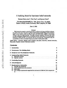
4. ARCHITECTURE AND IMPLEMENTATION The NAP system can be roughly divided into three main components: monitoring, analysis, and remediation. Figure 1 depicts the high-level architecture of NAP in a hypervisor environment. In this setting, the host runs two virtual machines, one of which is a service virtual machine running the NAP system and the other one is the virtual machine running an application. In order to service client requests, the application VM communicates with the outside world over a virtual network interface. All the network traffic of the server passes through the service virtual machine, where the NAP monitoring module collects the needed information. We note that having a special virtual machine handle all network traffic for other virtual machines is very common and is the default mode of operation for the Xen hypervisor [6], regardless of NAP. The overhead added by NAP is confined to the monitoring module’s overhead.
4.1 Monitor The application-agnostic feature of the monitoring system stems from the fact that the system observes the TCP/IP headers only and makes no assumptions about higher-layer protocols beyond the very general assumptions of Section 3.1. The monitoring module treats the packet incoming to the monitored server and containing some data (as opposed to headers only) as
Figure 1: NAP – high level architecture requests, and packets outgoing from the server and containing some data as responses. Packets belonging to the same request/response pair have the same sequence and acknowledgment numbers respectively. Therefore, no request or response is counted more than once. Additionally, the TCP packets of a request contain the acknowledgement number of the corresponding response, thus allowing the exact calculation of a request’s response time. The monitoring module is a light-weight packet sniffer, which is responsible for collecting traffic information such as the headers of data packets sent and received by clients during a monitoring interval ∆. The actual packets capturing is performed via the JPCAP library5 . The packet headers are processed online and the main statistics such as L, λ, T , W , and S are calculated for each ∆ as described in Section 3. The monitoring component is configurable, allowing the administrator to set a timeout after which an unanswered request would be either discarded or counted as request with a maximal response time Tmax . Other helpful (optional) parameters include: Filter String : specifies which ports should be monitored by NAP for this VM, e.g., "port 80"; Worker Thread Pool Size : number of worker threads configured at the server side. Currently, we obtain this information from the configuration files, e.g., from inspecting Apache MPM common directives. If these parameters are not set, as may be a common case in the black box model, NAP infers them from the out-of-band traffic monitoring. In particular, if the port that should be monitored at the virtual interface of a server VM is not specified, NAP monitors this interface in a promiscuous mode capturing all IP datagrams, 5 http://netresearch.ics.uci.edu/kfujii/ jpcap/doc/index.html
extracting the port numbers from the encapsulated TCP segments and listening to all ports with activity. If the maximal number of working threads is unknown, NAP performs a special test to estimate it. Namely, NAP chooses a request from the observed traffic, and sends it to the VM under the test at a constant rate, increasing this rate gradually. For these requests, NAP measures total average response time. When the number of worker threads becomes smaller than the number of requests that arrive simultaneously, some requests get queued. This is manifested by an increase in the average wait time and, consequently total average response time. NAP captures this change point to estimate the number of workers in the pool. The monitoring module of NAP works as follows. The monitoring module stores the key attributes of request and response TCP/IP segments headers such as arrival timestamp, sequence and acknowledgment numbers using internal data structure. Each response is matched with its request, or discarded after the maximal response time timeout, which is set to be a number of ∆-s. Consequently, ∆-s with the end time earlier then the current time − maximal response time are marked as “aged”. For the aged ∆, the monitoring module computes the values of S and W using Equations 1–4 and passes them to the analysis module. Eventually, the aged data is discarded. In the current version of NAP ∆ is manually set and it is not adaptive. However, a simple adaptive heuristic is possible to automate this process. Namely, let ε be a maximal error in the estimation of averages that we want to admit at the α confidence level. Then, window should is adaptively set in such a way that the number of requests (a) approximately equals the number of requests and (b) the number of request-response pairs in Z 2 the window n > (s · α/2 ε ) , where Zα/2 is the critical value of unit Normal variate at confidence level α and s is the sample standard deviation computed over the total response time measured for each request/response pair. Inability to determine ∆ that satisfies these conditions may in itself be an indicator of performance instability as the job flow in the system is highly unbalanced on every time scale. Another reason for inability to set good ∆ may be large sample standard deviation, which is indicative of significant differences between requests in the system. If this is the case, univariate datapoints clustering will be performed and then W and S will be computed per each cluster, as explained in Section 5.
4.2 Analysis and Remediation The analysis module stores the values of S, and W for a sliding time window comprising a number of ∆-s. Using the data in the sliding window, the distributions of S and W are calculated and compared to the corresponding baseline distributions. The comparison of the distributions is implemented as a pluggable component, which is easy to change and reconfigure. In the current version of NAP, the comparison algorithm is a simple percentile analysis, which is depicted in Algorithm 1. Based on the comparison results, the decision is made whether to raise a performance hot spot (or under-utilization) alarm. If an alarm is raised, the remediation module is engaged.
Input: baseS[ ], baseW[ ] : values of S and W in baseline; winS[ ], winW[ ] : measured S, W in a sliding time window; X : percentile; threshold : threshold percentage (between 0 and 1); Output: alert message percBaseS ← Xth percentile of baseS; percBaseW ← Xth percentile of baseW; percWinS ← Xth percentile of winS; percWinW ← Xth percentile of winW; if percBaseW·(1+threshold) < percWinW and percBaseS·(1+threshold) < percWinS then alert(“over-utilization – more resources per instance are needed”) ; return; end if percBaseW·(1+threshold)< percWinW then alert(“over-utilization – more instances needed”) ; return; end if percBaseW·(1-threshold) > percWinW and percBaseS·(1-threshold) > percWinS then alert(“under-utilization – less resources per instance are needed”) ; return; end if percBaseW·(1-threshold) > percWinW then alert(“under-utilization – less instances needed”) ; return; end Algorithm 1: Decision making algorithm
The third, remediation component, decides which (if any) action to take in order to remediate the problem detected by the analysis component. Remediation is usually done by either scaling-up the tier (i.e., adding more VM instances at that tier) or scaling-up (i.e., adding more resources to each instance) the service layer where the problem is detected. One of the advantages of the NAP system is that it can clearly indicate in which tier of the n-tier application the problem occurred and suggest the proper remediation action.
5. EXPERIMENTAL EVALUATION The primary purpose of our evaluation study is to usefulness of simple out-of-band black box traffic monitoring for detecting performance hot-spots reliably. In this initial study we leave some important questions out of the scope. First, our testbed is static and we do not evaluate NAP in a virtualized infrastructure environment that uses migrations. Second, we exclude network perturbations from our evaluation experiments. Third, we did not include hardware failures or software bugs into our evaluation scenarios. These issues are important and they are deferred to the future work. NAP was evaluated using two setups: (1) a synthetic client-server application tailored specifically to sanitycheck the model and gain intuition and (2) a real world
application simulation using Trade6. The synthetic application provided full control over the client workloads and the server-side application behavior. This simple application allows reproducing problematic serverside states and inspecting the monitoring system behavior before and after the problem remediation. After gaining intuition and acquiring insight with this simple system, we demonstrate that our approach works well for Trade6, which is considerably more complex. Our toy synthetic application consists of three VMs deployed on three different physical hosts: (1) client workload generator VM, (2) application server VM, and (3) database VM. There were two types of requests in our application: SELECT and UPDATE. With probability 50% clients invoke either SELECT or UPDATE. When received by the application server, both SELECT and UPDATE trigger a series of intensive I/O mixed with intensive calculations, which can heavily tax CPU. Processing SELECT requests takes approximately twice as long as processing the UPDATE requests. After finishing the calculations, the application server submitted an appropriate SELECT or UPDATE query to the second VM, which ran the PostgreSQL database server. On the DB server, the SELECT query again took approximately twice as long as the UPDATE command. The baseline workload was set for 30 users. Several executions (totalling 120,000 client queries) were performed with this workload. We measured the baseline mean service time (S), the mean queue time (W ), and the mean total response time (T ) on the application server VM and on the DB VM. Fig. 2 depicts the cumulative distribution function (CDF) for S, W , and T as measured on the application server during the baseline executions.
Figure 3: Application server – increased workload. Topmost chart – 40 users, bottom chart – 50 users total queue time exceeded some predefined threshold, the problem should be remediated by scaling-up the application server tier, i.e., by adding more application servers. Doubling the number of application servers and splitting the users equally between them, brings the measured T , S, and W very close to the baseline shown in Fig. 2. Scaling-up VMs resulted in less successful remediation since CPU was not the primary bottleneck in this case. Another way to see what happens in the system during this experiment that varies the number of users, while keeps the computational complexity of requests the workload constant, is to plot the S, T , and W times vs. the mean queue length L (see Eq. 1), as shown in Fig. 4. As expected, T and W in N exhibit a linear dependency on L, while the mean service time, S, stays constant.
Figure 2: Application server times CDF – baseline (30 users) In order to simulate a problematic state, we increased the number of users. Two additional experiments were conducted, in which the number of users was raised first to 40 and then to 50. Fig. 3 depicts the CDF of the times as measured on the application server VM during these two experiments. Increasing the workload to 40 and 50 users resulted in growth of the 95th percentile of the mean total queue time W by 55% and 111% respectively, compared to the baseline. It is important to notice that the service time S during the 3 aforementioned executions stayed approximately constant (this counter-intuitive situation was discussed in Section 3.3). Since the server’s mean service time did not change (it took the same time to complete a query as it took in the baseline), but the
Figure 4: Application server – times vs. queue length Another set of experiments was conducted to show NAP’s ability to detect the problematic states in a system where the client workload remains constant but some internal server problem occurs. For example, such a problematic state can be caused by a database which has grown too large, unexpected CPU load outside the system’s control, or insufficient disk bandwidth. In order to simulate such a problematic state, a new process running an endless loop of calculations was launched
on the application server VM. This resulted in heavy CPU load in the virtual machine bringing it up to 100% usage and, thus, severely degrading performance in the application server. The workload used in this run was the same baseline workload produced by 30 client threads as shown in Fig. 2. Fig. 5 depicts the measured times during the period of CPU overload. It is notable that the 95th percentile of all three measurements (S, T , and W ) increased by approximately 500%. This, naturally, was more than enough to trigger an alert.
Contrary to the application server, the DB server showed no serious fluctuations in the system responsiveness, as this VM was not affected during the experiment. On the DB VM, the queue time was zero during all runs, therefore S was always equal to T .6 To show the applicability of the NAP monitoring system to real-life complex applications, we tested NAP with the 3-tier IBM Trade6 application that simulates stock exchange trade environment. Trade6 consists of WebSphere Application Server, the DB2 database, and the Rational Performance Tester 6.1 application, which generates the client load. We used the default server and client configurations7 . This experiment was set up as follows: one VM running the WebSphere application server, a second VM running the DB2 database server, and two physical machines acting as clients. The application server (WebSphere) VM was initially configured to run with a single virtual CPU. Fig. 7 shows the CDF for the baseline time measurements, made during 15 minutes with a workload generated by 350 users.
Figure 5: Application server – CPU overload CDF In this case, both the mean queue time W and the mean service time S were much higher than the baseline. This can indicate either the increased difficulty of the workload (each query takes more time), or some internal misbehavior of the server (which, as we know, was the case due to controlled problem injection that we performed). In any case, the VMs in the problematic tier should be scaled up (each instance given more resources) in order to remediate the problem. In our setup, this was done by adding an additional virtual CPU. Fig. 6 depicts the measurements of the monitoring system after the problem remediation.
Figure 6: Application server – CDF after remediating CPU over-load The results of this run suggest that the system’s responsiveness has almost returned to normal. The measured times still show a degradation of 10-20% when compared to the baseline, but contrasted with the previous 500% degradation, this is a successful remediation. We note that performance degradation tolerance level is a configurable system parameter. In the current version of NAP, this parameter is controlled manually. If Service Level Objective (SLO) compliance for the application is being monitored and the compliance information is available to NAP, dynamic and adaptive threshold setting techniques can be used to automate threshold setting with controllable levels of false positive and false negative alerts [7].
Figure 7: Trade6 application server – baseline CDF In the next experiment, the number of users was increased to 600. Fig. 8 depicts the values of T , W , and S during the intensified workload as measured by NAP on the application server VM. It is notable that the 95th percentile of W increased by 154% while the 95th percentile of S stayed unchanged, suggesting that more application server instances are needed in the relevant tier. Expanding the application service tier by means of a new application server and redirecting half of the users to a new server resolves the problem and brings the system to a state that is nearly identical to the baseline. Another problematic state was simulated by means of an additional process, running an infinite loop on the Trade6 application server VM, which resulted in heavy CPU load. The CPU overload process is a multithreaded process where by controlling the number of computational threads, we controlled the overload level. Gradually increasing the number of threads resulted in proportional CPU load increase. Fig. 9 depicts the 6 It is reasonable to expect that under extreme load conditions the statistics NAP calculates for the DB tier may also be affected. For example, if the application server slows down to the point that transmission window would become zero often, NAP will assume that service time has increased. We were not able to create such adverse conditions, however. 7 The default configuration is described in http://www.ibm.com/developerworks/edu/ dm-dw-dm-0506lau.html.
Figure 8: Trade6 application server – increased workload CDF measurements for the maximal over-load level. In this state the mean queue time and mean service time are higher by approximately 121% and 48% compared to the baseline. This suggests that the remediation policy that allocates more resources to the application server is most likely to succeed.
Figure 9: Trade6 application server – CPU overload CDF
memory vs. accuracy. During our tests, the memory usage of the monitoring system implemented in Java was about 50MB. This memory usage also included packet capture library and an additional statistics library. This suggests good scalability even though an explicit scalability study was not performed at this stage. The main appeal of the percentile-based statistic analysis is its intuitiveness and simplicity. However, this approach should be exercised with caution in cases where requests differ dramatically making analysis of the CDF of mean values of S and W insufficiently sensitive. For instance, the aforementioned Trade6 application contains 15 different request types. The distributions of the number of these requests and their response time are presented in Fig. 11 and Fig. 12 respectively. Gradual CPU overloading of the Trade6 server showed that the performance of all the requests degraded almost equally as the load increased. However, for the sake of a thought experiment, let us assume that the “Trade Home” request would be the only CPU intensive request out of all the 15 request types, while the rest of the queries would be I/O intensive. In such case, doubling the CPU load on the Trade6 server will case 100% degradation for the “Trade Home” requests. Nevertheless, the 95th percentile of the mean total response time increases only by approximately 9% which may be not enough to trigger an alert. In such cases, the request-response data can be clustered, using algorithms such as X-means or PG−means [11, 12, 21, 23]. This is even an easier task than usual, since the data is univariate (using directly measured total response time). After clustering, data in each sub-cluster can be treated as a separate source of information exactly as presented above.
The remediation policy allocated virtual CPUs one by one, resulting in 4 total virtual CPUs allocated. Fig. 10 depicts the measured times after the problem remediation. As the graphs show, the mean service time and the mean queue time 95th percentiles are now nearly 16% and 29% lower then the respective baseline times.
Figure 11: Trade6 – requests count distribution
Figure 10: Trade6 application server – remediation CDF It is notable that during all of the experiments mentioned above, the average CPU utilization by the monitoring system was 0%. The memory consumption of the monitoring system depended on several parameters, such as number of deltas considered during the distribution calculations, the number of baseline measurements, and the maximal request time. These parameters could be tuned to achieve the right trade-off of
Figure 12: Trade6 – response time distribution
6. CONCLUSIONS We have presented a novel out-of-band performance management system NAP. Major features of NAP include application and protocol agnostic monitoring and
analysis, negligible performance overhead, accurate detection of hot spot tiers and of problematic VMs within these tiers, and an ability to trigger efficient remediation action in an autonomous manner. We evaluated NAP using the well accepted Trade6 benchmark with several types of workload. Our future research directions include: • Evaluating NAP with real production systems; • Evaluating and integrating NAP with a large scale, highly dynamic infrastructure cloud environment, where VM migrations are possible, such as RESERVOIR [22]; • Automatically learning – at the infrastructure level – of the elasticity rules that govern services capacity allocation decisions to satisfy fluctuations in demand in a cost-effective manner; • Evaluating our solution in presence of network problems and software bugs. We believe that wherever gray-box or white-box performance management is feasible, it is generally preferable over the black box one. However, there are many important settings, where gray-box or white-box approach is not applicable. As we show in this paper, in such cases NAP offers an attractive and powerful alternative.
7. REFERENCES [1] The Amazon Elastic Compute Cloud (Amazon EC2) web site. http://aws.amazon.com/ec2. [2] Gogrid. http://www.gogrid.com. [3] K. Appleby, S. Fakhoury, L. Fong, G. Goldszmidth, M. Kalantar, S. Krishnakumar, D. P. Pazel, J. Pershing, and B. Rochwerger. Oceano-SLA based management of a computing utility. IEEE/IFIP IM’01, pages 855–868, 2001. [4] B. Claise, Ed. Cisco Systems NetFlow Services Export Version 9, RFC3954, Oct 2004. [5] B. Claise, Ed. Specification of the IP Flow Information Export (IPFIX) Protocol for the Exchange of IP Traffic Flow Information, RFC5101, Jan 2008. [6] P. Barham, B. Dragovic, K. Fraser, S. Hand, T. Harris, A. Ho, R. Neugebauer, I. Pratt, and A. Warfield. Xen and the art of virtualization. In SOSP ’03, pages 164–177, New York, NY, USA, 2003. [7] D. Breitgand, M. Goldstein, E. Henis, and O. Shehory. Reducing Levels of Negative and Positive False Alarms via Multiple Adaptive Thresholds. In IFIP/IEEE IM’09, to appear, June 2009. [8] I. Cohen, M. Goldszmidt, T. Kelly, J. Symons, and J. S. Chase. Correlating instrumentation data to system states: a building block for automated diagnosis and control. In OSDI’04, pages 16–16, Berkeley, CA, USA, 2004. USENIX Association. [9] J. Coleman and T. Lau. Set up and run a Trade6 benchmark with DB2 UDB – IBM tutorial. http://www.ibm.com/developerworks/edu/ dm-dw-dm-0506lau.html.
[10] Distributed Systems Architecture Group at Universidad Complutense de Madrid. OpenNebula, 2008. [11] Y. Feng, G. Hamerly, and C. Elkan. PG-means: learning the number of clusters in data. In The 12-th Annual Conference on Neural Information Processing Systems (NIPS), 2006. [12] Greg Hamerly and Charles Elkan. Learning the k in k-means. In The 7th Annual Conference on Neural Information Processing Systems (NIPS), pages 281–288, 2003. [13] A. Gupta. Black Box Methods for Inferring Parallel Applications Properties in Virtual Environments. PhD thesis, EECS, Northwestern University, May 2008. [14] J. Hellerstein, T. Jayram, and I. Rish. Recognizing end-user transactions in performance management. In AAAI’00, pages 596–602, Menlo Park, CA, USA, 2000. AAAI Press. [15] S. Kato, T. Yamane, and T. Noagayama. Automated performance problem determination by observing service demand. Technical report, IBM Research, Tokyo Research Lab, 2007. [16] A. Lakhina, M. Crovella, and C. Diot. Mining Anomalies Using Traffic Feature Distributions. In SIGCOMM’05, pages 217–228. ACM, 2005. [17] Little, J. D. C. A Proof of the Queuing Formula L = λ W. Operations Research, 9(383–387), 1961. [18] M. A. Munawar, M. Jiang, and P. A. S. Ward. Monitoring Multi-Tier Clustered Systems with Invariant Metric Relationships. In SEAMS ’08, pages 73–80, New York, NY, USA, 2008. ACM. [19] G. Münz and G. Carle. Real-Time Analysis of Flow Data for Network Attack Detection. In IFIP/IEEE IM’07, May 2007. [20] D. Pelleg, M. Ben-Yehuda, R. Harper, L. Spainhower, and T. Adeshiyan. Vigilant: out-of-band detection of failures in virtual machines. SIGOPS Oper. Syst. Rev., 42(1):26–31, Jan 2008. [21] D. Pelleg and A. Moore. X-means: Extending K-means with efficient estimation of the number of clusters. In ICMLA’00, pages 727–734, San Francisco, 2000. Morgan Kaufmann. [22] B. Rochwerger, D. Breitgand, E. Levy, A. Galis, K. Nagin, I. Llorente, R. Montero, Y. Wolfsthal, E. Elmroth, J. Caceres, M. Ben-Yehuda, W. Emmerich, and F. Galan. The RESERVOIR Model and Architecture for Open Federated Cloud Computing. IBM Systems Journal, 2009. to appear. [23] T. Sherwood, E. Perelman, G. Hamerly, and B. Calder. Automatically characterizing large scale program behavior. In ASPLOS’02, 2002. [24] The Open Group. Application Response Measurement — ARM, 4.0 Version 2. http:// www.opengroup.org/management/arm/, 2007. [25] T. Wood, P. Shenoy, V. Arun, and Y. Mazin. Black-box and Gray-box Strategies for Virtual Machine Migration. In USENIX NSDI’07, pages 229–242, 2007.