NCR: A UNIFYING PARAMETER TO CHARACTERIZE AND EVALUATE DATA DISSEMINATION SCENARIOS, AND ITS ANALYTIC STUDY Biao Zhou, Mario Gerla Computer Science Department, UCLA, CA 90095, USA zhb,
[email protected] ABSTRACT Nowadays data dissemination often happens in vehicular sensor networks (VSN) and other mobile ad hoc networks in military & surveillance scenarios. For example, VSN is usually used to proactively monitor urban environment. In VSN, each sensor can generate a large amount of data which must be reliably reported to actuator agents. Data dissemination in conjunction with efficient harvesting has been proven to be very effective in this type of applications. The performance depends on many different parameters including speed, motion pattern, node density, topology, data rate, and transmission range. This multitude makes it difficult to accurately evaluate and compare data gathering protocols implemented in different simulation or testbed scenarios. In this paper, we introduce Neighborhood Change Rate (NCR), a unifying measurement for different motion patterns used in epidemic dissemination, a contact-based data dissemination. By its intrinsic property, the NCR measurement is able to describe the spatial and temporal dependencies and well characterize a dissemination/harvesting scenario. We illustrate our approach by applying the NCR concept to MobEyes, a lightweight data gathering protocol. We further analytically studied the effective NCR for Markov type motion models, such as Real Track mobility model. A closed-form expression has been derived. From this analytic solution, the NCR can be approximated from the initial scenario settings, such as velocity range, transmission range, and real map/street information. The closed-form formula for NCR can be further employed to evaluate the ED process. The mathematical relationship between the dissemination index and the effective NCR is established and it allows predicting the performance of the ED process in realistic track motion scenarios. The experiment results showed that the analytic expressions for the NCR and for the evaluation of the ED process closely match the discrete-event simulations. I. INTRODUCTION Dissemination has shown to be the most efficient way to transmit the seed of life. As a matter of fact, humans must deal with dissemination on a daily basis. The best known example is virus dissemination. When a human is contaminated by a virus and passively carries it, the virus is transmitted to other people whom he encounters. This kind of epidemic transmission is very efficient since human mobility and human density contribute to make it virtually unstoppable. The close similarity between human virus carriers and routers in a data network has become a source of inspiration for characterizing digital dissemination techniques. Data dissemination occurs in the course of the useful life of the data when the originator comes in contact with intended destinations. Such contact-based data dissemination is also known as “epidemic” dissemination (ED). In epidemic dissemination the
origin node periodically transmits the data (or metadata) to each current neighbor with a certain probability. In some cases, secondary relay from neighbors can also be performed, up to a scope (i.e., number of relay episodes). By analogy with the dissemination of human virus, node mobility is a clear aid to epidemic dissemination, even over sparse networks. Data dissemination is applied in a variety of fields. For geographic routing, data dissemination helps to propagate node geographic locations in the network, therefore relaxing the requirement for a centralized location server [1]. In delay tolerant networks (DTN), data dissemination is particularly efficient to convey information over sparse networks with high reliability [2]. In vehicular sensor networks (VSN) where vehicles are equipped with on-board sensing devices, data dissemination has showed to be especially efficient in maintaining a distributed index for data harvesting and forensic investigation [3][4]. Data dissemination is also applied in military and surveillance scenarios. Evaluating the efficiency of data dissemination is a key to estimate the performance of protocols that rely on it. The performance of data dissemination depends on many different parameters including speed, motion pattern, node density, topology, data rate, and transmission range. This multitude makes it difficult to accurately evaluate and compare data gathering protocols implemented in different simulation or testbed scenarios. Evaluating protocols based on multi-criteria is hard, which often yields to inconsistent results, so reducing the “control panel” to a small set of independent parameters helps to facilitate the fair comparison of protocols. Studies in epidemic dissemination have shown that the performance of data dissemination is closely affected by node motion pattern and node density [3]. Although node density is a rather straightforward measure to define, node motion pattern is much more difficult to characterize. There are many motion patterns proposed and each of them is composed of different parameters. So far no unifying criteria are proposed to characterize motion patterns and to evaluate the data dissemination process uniformly. In this paper, we introduce Neighborhood Change Rate (NCR), a unifying measurement for different mobility models used in epidemic dissemination. NCR is based on the rate of node entering and leaving a neighbor set. We will illustrate how NCR has a significant influence on the performance of data dissemination. Coupled with velocity and density, NCR is shown to fully describe the data dissemination process. We illustrate our approach by applying the NCR concept to MobEyes [3], a lightweight data gathering protocol. We further analytically studied the effective NCR for Markov type motion models, such as Real Track mobility model. A closed-form expression has been derived. From this analytic solution, the NCR can be approximated from the initial scenario
1 of 8
settings, such as velocity range, transmission range, and real map/street information. The closed-form formula for NCR can be further employed to evaluate the ED process. The mathematical relationship between the dissemination index and NCR is established and it allows predicting the performance of the ED process in realistic track motion scenarios. We conduct discreteevent simulations and compare the experiment results with the analytic results from the closed-form solutions of NCR and the ED process. The rest of the paper is organized as follows. Section II gives an overview of mobility models used in epidemic dissemination. In Section III, we introduce the NCR and its illustration by MobEyes simulations. Section IV describes the analytic study of NCR and its validation and comparisons by discrete-event simulations, and we conclude the paper in Section V. II. MOBILITY MODELS IN EPIDEMIC DISSEMINATION Mobility has a determining impact on epidemic dissemination due to longer term topology disconnection episodes. Preliminary results, reported in [3], show that there is a very strong dependence between event harvesting and motion pattern. For example, if we assume that vehicles move in a random motion pattern known as Random WayPoint model [5], the collection of nearly all events is one order of magnitude faster than with realistic motion constrained by urban traffic consideration (the Track motion model [6]). So studies on realistic mobility models and studies on the impact of mobility pattern on data dissemination are needed. The Random Waypoint (RWP) mobility model is one of the most widely used motion models for MANET scenarios. In the RWP model, a node randomly selects at each interval a new direction [5]. Random Walk and Random Direction models provide more realism than RWP [7][8]. The Obstacle mobility model proposed in [9] extends the RWP model through the incorporation of obstacles using a Voronoi diagram of obstacle vertices. In the Manhattan mobility model proposed in [10], the mobile node is allowed to move along the horizontal or vertical streets. At each intersection, the node can turn or go straight with certain probabilities. Some of the above random models reflect the urban topology, but none of them are inadequate to model motion correlation among vehicles. Nodes in vehicle networks tend to form “convoys”. There is some individual random movement, but there are also factors that tend to introduce strong correlation between individual trajectories, for example, obstacles, traffic accidents, traffic lights, etc. To capture the most representative features of urban motion, we proposed a “track” group motion model based on a Markov Chain approach [6]. The tracks are represented by freeways and local streets. The group nodes must move following the tracks. At each intersection, a group can be split into multiple smaller groups; or may be merged into a bigger group. The track model allows also individually moving nodes as well as static nodes. The latest version is called Real-Track (RT) mobility model which is tested with real freeway/street maps from the US census bureau. Similar work is done later by [11], which focuses on multi-level human mobility heterogeneity in local community though. As we mentioned before, mobility pattern has a critical impact on the performance of epidemic dissemination. But how to
evaluate the influence of mobility patterns is a key challenge. There are many motion models proposed and each of them is composed of different parameters. So far no unifying criteria are proposed to characterize motion patterns and to evaluate the data dissemination process uniformly. That is the motivation we introduce the NCR (Neighborhood Change Rate) measurement which characterizes motion patterns and allows us to predict the performance of an ED process. III. NCR 3.1 Factors Affecting the Efficiency of Data Dissemination The efficiency of data dissemination can be briefly defined as the total time needed to spread a given set of data to the entire network. Similarly to virus spreading, the larger set of vehicles a car meets per encounter point, the more efficient is the data dissemination in VSN. But group motion doesn’t help the data dissemination. Indeed, the data dissemination efficiency can be increased if the cars met at the encounter points do not follow a similar trajectory as the data bearer. On the other hand, in epidemic dissemination each encounter point is an opportunity for nodes to spread data to other nodes. The high frequency a car encountering other cars helps the data dissemination. Therefore, the efficiency of data dissemination is dependent on two major factors: 1) the number of vehicles with different trajectories a car met per encounter-point; and 2) the frequency a car encountering other cars. However, the above two criteria are neither uncorrelated nor atomic. In other words, they are both composed of, and potentially share, a multitude of parameters, such as velocity, density, node distribution pattern, or driving patterns, etc. 3.2 NCR Definition NCR, Neighborhood Change Rate, is a comprehensive measurement which combines the above two major affecting factors together and provides a good evaluation of epidemic dissemination. Simply speaking, NCR is the rate of change of nodes in one’s transmission radius. Its definition is as follows:
NCR i (t + ∆t ) =
[
] [ ] [
]
i i E # Nbleave (∆t ) + E # Nbnew (∆t ) (1) i i E Deg (t ) + E # Nbnew (∆t )
[
]
Where ∆t is the sampling interval which is equal to the time needed for a node to travel the distance of its transmission range; i E # Nbnew ( ∆t ) is the expected number of nodes entering node
[
]
i ∆t ; E [# Nbleave ( ∆t )] is the expected number of neighbors leaving node i’s neighborhood during ∆t ;
i’s neighborhood during
and Deg i (t ) is the nodal degree of node i at time t. Fig. 1 depicts the evolution of the NCR computed for the car C1. At time t-3, NCR(t-3)=0 as C1 did not encounter any other cars yet. At time t-2, NCR(t-2)= 1/2, as C1 met C2 as new neighbor. And at time t-1, NCR(t-1)=2/3, as C1 lost and gained a neighbor. Someone might argue that at time t-1 car C1 had only one encounter and gained one neighbor so the capacity of data dissemination should be similar to the previous case at time t-2. However, at time t-1, C1 also released C2 which would also spread the information to other nodes. So NCR(t-1) is higher than NCR(t-2). Finally, at time t, C1 released C4 and reached its maximum diffusion, and the calculation result of NCR(t) is 1.
2 of 8
In order to illustrate the effect of NCR, we have performed a range of simulations on MobEyes [3] which is an efficient lightweight support for proactive urban monitoring based on the primary idea of exploiting vehicle mobility to opportunistically diffuse summaries of sensed data. The core of MobEyes is MobEyes Diffusion/Harvesting Processor (MDHP). The MDHP has a dual role to play: summary diffusion where private vehicles opportunistically and autonomously spread summaries of sensed data by exploiting their mobility; and summary harvesting used by agents (such as police cars) to proactively build a low-cost distributed index of the mobile storage of sensed data.
Fig. 1. The NCR of Car C1 as a function of time ( ∆t =1). 3.3 NCR Properties From the above definition and description of NCR, we easily know that NCR is a ratio with the property of 0≤NCR≤1 since the number of leaving nodes will never bigger than the nodal degree of the node. Another property is that NCR is independent of average speed and average density in scenarios with uniformly distributed velocities and node positions. In NCR definition, ∆ti is dependent of velocity vi, but if speed decay from the average speed is negligible, ∆t1≈∆t2. In a scenario with uniformly distributed velocii i ties and node positions, # Nbnew ≈ # Nbnew and / leave ( ∆t 2 ) / leave ( ∆ t1 )
In these simulations, we are interested in the diffusion latency as a function of speed and the harvesting efficiency as a function of time under different NCRs. We also perform the cross comparisons among different motion patterns and different topologies for similar NCR. In the simulations, we applied a realistic mobility model, the real-track (RT) model [6] on the urban map topology (Westwood map) shown in Fig. 2. We evaluate the performance by randomly choosing 10 harvesting agents and repeat running 30 times to get a smooth curve. The simulation parameters are shown in Table 1. Table 1. Simulation Parameters. Simulator Simulation time Simulation Area Number of Nodes Number of Agents Number of Runs Speed Radio Range Pause Time
Deg i (∆t1 ) ≈ Deg i (∆t2 ) . Thus, NCR will not change with average
speed. Average density is defined as the average number of neighbors per node per covering area. In scenarios with uniformly distributed velocities & positions and fixed transmission i i range, densityavg ≈ Deg i (t ) and densityavg ≈ densityavg , where i is the average density around node i and densityavg is densityavg the average density for the whole scenario. As we normalize NCRi (t ) with Deg i (t ) , NCR is independent of densityavg .
NS-2.27 2000s 2400m x2400m grid 100 10 30 5m/s→25m/s 250m 0s
The above NCR property may be intuitively illustrated by the possibility of obtaining different NCRs for the same average velocity or density. Moreover, as shown in Section 3.4, data disseminations with different NCRs but with same average speed and density have different performance. It fosters the justification for NCR as an appropriate parameter which models temporal and spatial dependencies and other mobility patterns that cannot be described by average speeds or velocities. But in reality it is not easy to give a specific NCR value since it is an evolution value changing with time. Instead we use low, medium and high NCR to distinguish different scenarios having different motion patterns, topology, street layouts, radio range, and node distributions. A similar situation exists in Transportation Planning. How to represent traffic flows in transportation depends on multi-parameters, such as speed, density, and volume/capacity, etc. The transportation community defined the Level of Service (LOS). It works like a grade of report card, using the letters A through F with A being best and F being worst. By using LOS classification and referring to a traffic situation with a particular LOS, engineers can have a global knowledge of traffic condition in a particular area. NCR is designed to have the same usage as LOS. By referring to a data dissemination in specific scenario with a particular NCR (low, medium, or high), we can have an intuitive vision of its data dissemination efficiency, and thus evaluate VANET protocols using this feature. 3.4 NCR Illustration by Simulations of MobEyes
Fig. 2. Westwood Map Topology. As we mentioned in Section 3.3, we use low NCR, medium NCR, and high NCR to feature different sets of motion patterns. Fig. 3 shows diffusion latency as a function of velocity under different NCRs in the scenarios of map topology with track motion pattern. As we expect, the latency drops with the increase of speed. Moreover, the latency is determined by the NCR feature for the same speed. For example, when the speed is fixed as 5m/s, the delay is 1250s for low NCR, but drops to 850s and 640s for medium NCR and high NCR respectively. The performance is improved as the NCR increases. As we normalized the results with the density, the improvements come from the particular motion characteristics other than speed or density, such as group effect (temporal and spatial dependencies) for the Track model, or the urban-grid restriction in the map topology
3 of 8
(spatial dependencies). NCR exactly catch the above motion features.
1
Harversting efficiency [%]
0.9
1300
High NCR Medium NCR Low NCR
1200 1100
Delay [s]
1000 900 800 700
0.8 0.7 0.6 0.5 0.4 0.3 0.2 High NCR, speed=15m/s Medium NCR speed=15m/s Low NCR speed=15m/s
0.1
600
0 0
500
500
1000
1500
2000
Time [s]
400 300 5
10
15
20
(b) Average velocity = 15 m/s
25
Average velocity in [m/s] 1
Fig. 3. Diffusion latency as a function of speed.
0.9
1
Harversting efficiency [%]
0.9 0.8 0.7 0.6 0.5 0.4 0.3 0.2 High NCR, speed=5m/s Medium NCR speed=5m/s Low NCR speed=5m/s
0.1 0 0
500
1000
1500
Time [s]
(a) Average velocity = 5 m/s
2000
Harversting efficiency [%]
In Fig. 4, we illustrate the harvesting efficiency rate as a function of time in the track motion scenarios with map topology for different average velocities of 5,15,25 m/s. Fig. 4 shows that that the higher NCR increases the harvesting efficiency. For example, in Fig. 4(a), after 1000s, MobEyes has harvested 95% of the events for the high NCR, but only 90% and 70% for the medium and low NCR respectively. Similar effects are seen in Fig. 4(b) and 4(c). But if we compare Fig. 4(a), (b) and (c), we can see that the high-level NCR has less impact when average speed increases. This may be intuitively explained by the fact that an increased speed reduces the spatial and temporal dependencies created by different topologies, as faster nodes are less subject to the effect of urban-grid restriction in map topology: they reach their targets quicker and then move again on a different path.
0.8 0.7 0.6 0.5 0.4 0.3 0.2 High NCR, speed=25m/s Medium NCR speed=25m/s Low NCR speed=25m/s
0.1 0 0
500
1000
1500
2000
Time [s]
(c) Average velocity = 25 m/s Fig. 4. Harvesting efficiency as a function of time. To do the cross comparisons among different motion patterns and different topologies for similar NCR, we chose the steadystate Random Waypoint model on graphs [12] as a comparing motion pattern and chose a simple triangle topology with equal edge of 760m as a comparing topology. Fig. 5 shows the simulation results which has been normalized by the average density to remove the influence of the density. From Fig. 5(a) and (b), we can see that the performance of data dissemination is almost identical in the scenarios with similar NCR, speed and density. For example, in Fig. 5(b), although the harvesting processes slightly differ during the simulation, they are completed at roughly the same time. From Fig.5(a), the latency is also similar for all three cases, just a few seconds time difference. This well shows the significance of NCR, as it is able to characterize the intrinsic properties of complex topologies or motion patterns and feature the complex spatial and temporal dependencies observed in realistic mobility patterns.
4 of 8
N N Ci , j
40
MAP Triangle RWM
35
E ( IRT ) =
Harvesting delay [s]
30
Σ Σ Σ Tk
i =1 j =1 k =1 N N
(2)
Σ Σ Ci , j
i =1 j =1
25
N N
20
NCReff =
15
Σ Σ Ci , j
i =1 j =1 N N Ci , j
(3)
Σ Σ Σ Tk
i =1 j =1 k =1
10
where N is total number of nodes in the system; Ci, j is # of changes from in range to out of range for pair (i, j); and Tk is the kth In Range Time (IRT) for pair (i, j).
5 0 10
15
20
25
Speed [m/s]
From Equation (2) and (3), we can get: (a) Delay
NCReff ∝
1
Harversting efficiency [%]
0.9
1 (4) E ( IRT )
From the new definition (3), we briefly know that NCReff, the effective NCR, is now an encountering frequency over in range time.
0.8 0.7 0.6
4.2 General Approach to Get NCReff
0.5
Obviously, if we get E(IRT), we can easily obtain NCReff by inversing the E(IRT). The general approaches of the average link duration E(LD) [13][14][15] can help us to get E(IRT). Indeed, E(IRT) and E(LD) are two different views for the same measurement: E(IRT) is from the view of pair in range, which composes a link; and E(LD) is from the view of link, which means that a pair is in their transmission range.
0.4 0.3 0.2 MAP NCR, speed=15m/s Triangle NCR speed=15m/s RWM NCR speed=15m/s
0.1 0 0
10
20
30
40
50
60
70
Time [s]
(b) Harvesting efficiency. Fig. 5. Cross comparison of different motion patterns and topologies for similar NCR. In summary, NCR is a unifying parameter, as it re-groups mobility patterns and topology parameters. NCR is able to describe spatial and temporal dependencies which are not covered by speed or density. Coupled with the average speed and the average density, NCR can well evaluate the process of data dissemination. IV. ANALYTIC STUDY OF NCR The goal of the analytic study of NCR is to get a closed-form expression for data dissemination under realistic motion pattern, such as real track model with map topology. 4.1 Definition of NCReff As mentioned in section 3.3, we can only get a “grade” level of NCR. To get an analytic solution for NCR, we need to re-define NCR and we call it as NCReff, i.e., effective NCR. We first introduce the definition of Average In Range Time E(IRT). IRT (In Range Time) is defined as the time duration when a pair of nodes is within their mutual transmission range. To simplify the problem, our assumption is that in the initial node distribution we put nodes one by one into an initially empty system. Then E(IRT) and NCReff can be defined as follows:
The major steps of obtaining NCReff are as follows: 1) State space derivation for Markov motion models; 2) Derive probability transition matrix; 3) Derive separation probability vector after k epochs; 4) Derive general expression of E(IRT) by studying relative movement between two randomly moving nodes and conditional PDF (Probability Density Function) of separation distance; 5) Apply the general expression of E(IRT) to different Markov mobility models, and make approximations for each model to get a closed-form expression for E(IRT); and finally 6) inverse E(IRT) to get NCReff. We briefly introduce the basic concept of each step here, and the details can be obtained in [14] [13]. In Markov motion models, such as track mobility model [6] or random walk mobility model [7], the evolution of the separation distance between two nodes is a Markov process. The probability density function (PDF) of Lm+1 is only dependent on Lm, where Lm is the separation distance between two nodes at epoch m and lm is an instance of Lm. Thus, the state space E = {e1 , …, ei , …} in Markov motion models can be determined by the separation distance between a pair of nodes. The node separation distance is divided from 0 to r (i.e., radio range) into n bins of width ε. Lm is in state ei if (i-1)ε ≤ lm < iε. The probability transition matrix A is then shown as follows:
5 of 8
a1,1 .L a1,n M O M A= an ,1 L an ,n 0 L 0
a1,n+1 M (5) an,n+1 1
4.3 NCReff in Track Mobility Model For Markov Chain models, transition probability ai,j in (5) is derived from the conditional PDF of separation distance fLm+1|Lm(lm+1|lm). The detailed formula is shown below: jε
ai , j = Pr (ei → e j ) = P(lm +1 ∈ e j | lm ∈ ei ) =
iε
∫ ε ∫ εf
( j −1) ( i −1)
Lm+1 | Lm
(lm +1 | lm ) f Lm (lm )dlm dlm +1
(6) Using the properties of Markov chain models, the separation probability vector after k epochs is:
We are interested in the NCReff in the track mobility model as we try to analytically study the data dissemination process under a realistic motion pattern where vehicles are moving along streets in the real map. [15] gives an approximation for E(LD) (i.e., E(IRT)) in Random Walk (RW) model (shown in (14)) by applying the above approach in Section 4.2 to RW mobility model, a Markov mobility model.
P(k) = P(0) Ak (7) where P(k) is the probability vector of the node separation distance at k epoch; A is the probability transition matrix shown in (5); and P(0) is initial probability vector of the node separation distance, and its formula is shown in (8).
P(0) = [p1(0) p2(0)… pi(0)… pn(0) pn+1(0)] (8) where pi(0) is the initial probability that the node separation distance is in state ei . From [13], we know that the Probability Mass Function (PMF) of the link duration or the in range time is pn+1(k) – pn+1(k-1) and E(IRT) can be calculated as (9). n
n
i =1
j =1
E ( IRT ) ≈
where r is the radio range; v is the average speed, and the variance of the velocity v.
is
To catch the features of the track motion pattern and the map topology, we give the following definitions:
Pwithin =
The definition of F is as follows:
σ v2
The above approximation gives us a good hint which helps us to study the NCReff in track model. To simplify the problem for the track model with map topology, we assume that 1) Streets/roads in map are randomly and uniformly distributed; 2) Group size is 1 and nodes are randomly and uniformly distributed.
E ( IRT ) = ∑ pi (0)∑ Fi , j (9) where pi(0) is from initial probability vector P(0); and Fi,j is from Fundamental Matrix F.
v (12r − v ) (14) 9(v 2 + σ v2 )
v (15) Ls
where Pwithin is the probability that node is within a road but not in the intersections after one epoch (unit time); v is the average speed; and L s is the average road length in the map. If
L s is
F= (In - Q) (10)
Pwithin is greater than 1, we set it as 1. The calculation of shown in (16).
where In is an n×n identity matrix; and Q is derived from probability transition matrix A, and its definition is shown in (11).
Ls =
a1,1 L a1,n Q = M O M (11) an,1 L an,n
where TL is total road length; and TI is total number of roads. The Tiger/Line map data file from US Census Bureau will help us to calculate (16).
-1
where
TL (16) TI
We use Rptn to show the restriction of urban grid. Its definition is as follows:
ai , j is transition probability from A.
From (4)-(11), we know the following relationship:
R ptn =
f Lm+1 | Lm (lm +1 | lm ) → ai , j → A → Q → F → E ( IRT ) → NCReff
where Rptn is the ratio of urban grid restriction; Afree is ¼ of free
(12) NCReff is now determined by the conditional PDF of separation distance fLm+1|Lm(lm+1|lm) , which is normally determined by the fX(x), the PDF of relative movement between two nodes from epoch m to m+1 [14] [15]. The relative movement between two nodes usually depends on the mobility model being used. In summary, we have the following relationship:
Afree (17) Agrid
space area (i.e., whole field); and in the map. The calculation of
Agrid =
Agrid is the average grid area
Agrid is shown in (18).
TA (18) TG
where TA is total area of all urban grids; and TG is total number of grids. The grid data is also from US Census Bureau.
f X ( x ) → f Lm+1 | Lm (lm +1 | lm ) → ai , j → A → Q → F → E ( IRT ) → NCReff
(13) So our job is to feature different Markov mobility models to get the fX(x), make approximations for each model to get a closedform expression for E(IRT), and finally inverse E(IRT) to get NCReff.
Then we can get f x′( x) , the PDF of relative movement between two nodes in track model with map topology:
6 of 8
f x′( x) = (1 − Pwithin ) f x ( x) + ( Pwithin )( R ptn ) f x ( x) (19)
where f x ( x) is the PDF of relative movement of two nodes in RW mobility model. The simple explanation of (19) is that with (1-Pwithin) probability, node is in the intersections after one epoch, which relative movement is similar as in RW model because the roads are assumed to have a random and uniform distribution, but with Pwithin probability, the relative movement of two nodes will be restricted by the urban grid created by street maps. Based on (13), (14) and (19), we can have our approximation formula for E(IRT) in the track model with map topology:
ct v t (12r − vt ) (20) 2 9(vt + σ v2t )
E ( IRT )t ≈
where r is the radio range;
ct is track coefficient which
ct = (1 − Pwithin ) + Pwithin R ptn (21) We assume that in track model the range of group velocity is [0, Vgmax] and the range of individual velocity is [0, Vimax]. Since group velocity and individual velocity are two independent random variables, the expectation and the variance of Vt are as follows:
vg max + vi max
σ v2 = t
2 v g2 max 12
(22)
N − µ /λ (26) 1 + ( N − I 0 − µ / λ ) e − ( λN − µ ) t
Back to our systems with track motion pattern & map topology, µ = 0 here since we assume that no nodes will leave the system during the simulation. By the definition of NCReff in (3), we can easily know that the effective NCR, the encountering frequency over in range time, is proportional to λ, the meeting rate among peers. Thus, we have the following relationship:
λ = cλ NCReff (27) where cλ is a coefficient between λ and NCReff. By (26), (27) and the fact µ = 0, the dissemination index I(t) in the track motion scenario with a map topology can be derived by NCReff shown in (28):
I (t ) =
N −( c NCR N ) t 1 + ( N − I 0 )e λ eff
(28)
In summary, by (24) we get an approximation solution for NCReff in the track motion scenarios with a map topology, and by (28) we get a closed-form relationship between dissemination index and NCReff for data dissemination process under realistic motion pattern, i.e., real track motion model with map topology. 4.5 Experiment Validation and Comparisons
+
2 i max
v (23) 12
Thus, from (15)-(23) we get E(IRT), and by (4) we can get the NCReff in the track model with the map topology shown in (24).
9(vt + σ v2t ) 2
NCReff ≈
I (t ) =
vt is the average speed; and σ v2t is
the variance of the velocity vt ; and calculation is shown in (21).
vt =
The above differential equation (25) is separable and can be solved with the initial condition I0 (i.e., the number of sources at the beginning). Its solution is shown in (26).
ct v t (12r − vt )
(24)
The discrete-event simulations on MobEyes are conducted to validate and compare the analytic solutions in Section 4.3 and 4.4. In these simulations, we focus on the dissemination index (number of infected peers) as a function of time under realistic scenarios running the real-track (RT) model on the Westwood map topology shown in Fig. 2. The simulation parameters are shown in Table 2. Table 2. Simulation Parameters. Simulator Simulation time Simulation Area Number of Nodes # of Initial Source I0 # of Interested Peers N Speed Radio Range Pause Time
4.4 Apply NCReff to Evaluate Epidemic Dissemination Our basic goal of ED evaluation is to find how fast an index (or a file) spreads under a realistic and dynamic environment. We assume that there are N nodes interested in downloading the index. Let λ denote the rate of rendezvous (i.e., meeting) among those peers and µ denote the rate of departing the system (or content sharing area) respectively. As stated above, the meeting rate can be analytically driven [16] or empirically calculated [17]. We model this by using a simple epidemic model used in [18]. Let I denote the number of infected peers (i.e., those who have the index file). A single infected node meets other susceptible nodes (i.e., nodes without an index) with rate λ(N-I). Since I infected nodes are independently infecting others or leaving the system, the total rate of infection and departure is λ(N-I)I and µI respectively. Since the rate of change solely depends on the total meeting rate, we have the following expression:
I& = λ ( N − I ) I − µI (25)
QualNet 3.7 1600s 2400m x 2400m grid 300 1 300 10m/s→30m/s 375m 0s
Fig. 6 shows the comparisons between analytic results and simulation results for different max speeds of 10m/s, 20m/s and 30m/s. Analytic results perfectly match the simulation results with high speed and at long simulation time (shown in Fig. 6 (b) and (c)). Analytic results are lower than the results obtained in the beginning of simulations. The possible reason is that the analytic results are based on an initial distribution of an unbounded free space, which is not realizable in the simulation. The current simulation field is a bounded area of 2400m×2400m. Thus, the differences of the initial distribution condition between analytic solution and discrete-event simulation affect the results in early
7 of 8
stages. Fig. 6 (a) shows the worst match among these three figures. The possible reason is that the urban-grid restriction in scenarios with low speed is more pronounced than other scenarios with higher speed, as nodes in Fig. 6 (a) are more often trapped in urban grids. But the restriction of urban-grid is not easy to be exactly expressed by an analytic formula. But generally speaking, the experiment results in Fig. 6(a), (b) and (c) showed that the analytic expressions for NCR and for the evaluation of ED process closely match the discrete-event simulations. 300
Number of Infected Peers
250
200
150
100
Analytic Results 50
Simulation Results
0 0
200
400
600
800
1000
1200
1400
V. CONCLUSIONS We propose NCR (Neighborhood Change Rate), a unifying parameter which regroups mobility patterns and topology parameters in epidemic dissemination. By its intrinsic property, the NCR measurement is able to describe the spatial and temporal dependencies and well characterize a dissemination/harvesting scenario. The MobEyes simulation results well illustrate the effect of NCR. We further analytically studied the effective NCR for Markov type motion models, such as Real Track mobility model. A closed-form expression has been derived. From this analytic solution, the NCR can be approximated from the initial scenario settings, such as velocity range, transmission range, and real map/street information. The closed-form formula for NCR is further employed to evaluate the ED process. The mathematical relationship between the dissemination index and the effective NCR is established and it allows predicting the performance of the ED process in realistic scenarios under track motion patterns with map topology. The MobEyes experiment results showed that the analytic expressions for NCR and for the evaluation of the ED process closely match the discrete-event simulations.
1600
Time (seconds)
REFERENCE
(a)Max Speed = 10 m/s, cλ=0.035, NCReff = 3.06E-3, λ = 1.07E-4 300
Number of Infected Peers
250
200
150
100 Analytical Results
50 Simulation Results
0 0
500
1000
1500
Time (seconds)
(b)Max Speed = 20 m/s, cλ=0.035, NCReff =3.43E-3, λ = 1.20E-4 300
Number of Infected Peers
250
200
150
100
50
Analytical Results Simulation Results
0 0
200
400
600
800
1000
1200
1400
1600
Time (seconds)
(c) Max Speed = 30 m/s, cλ=0.05, NCReff = 3.63E-3, λ = 1.81E-4 Fig. 6. Analytic Results vs. Simulation Results.
[1] M. Grossglauser and M. Vetterli. Locating Mobile Nodes With EASE: Learning Efficient Routes From Encounter Histories Alone. In IEEE/ACM Transaction on Network, pp. 457-469, Vol. 14, NO. 3, June 2006. [2] W. Zhao, M. Ammar, and E. Zegura. A Message Ferrying Approach for Data Delivery in Sparse Networks. In MobiHoc 04, Tokyo, Japan, May 2004. [3] Uichin Lee, Eugenio Magistretti, Biao Zhou, Mario Gerla, Paolo Bellavista, Antonio Corradi. MobEyes: Smart Mobs for Urban Monitoring with a Vehicular Sensor Network. In IEEE Wireless Communications, Vol. 13, No. 5, Sep. 2006. [4] K.K. Leung. MESSAGE (Mobile Environmental Sensor System Across a Grid Environment) project. www.commsp.ee.ic.ac.uk/~wiser/message/. [5] D.B. Johnson and D.A. Maltz. Dynamic Source Routing in Ad Hoc Wireless Networks. In Mobile Computing, Chapter 5, pp. 153-181, Kluwer Publishing Company, 1996. [6] Biao Zhou, Kaixin Xu, and Mario Gerla. Group and Swarm Mobility Models for Ad Hoc Network Scenarios Using Virtual Tracks. In MILCOM ’04, Monterey, USA, October 2004. [7] T. Camp, J. Boleng, and V. Davies. A Survey of Mobility Models for Ad Hoc Network Research. In Wireless Communication and Mobile Computing (WCMC): Special issue on Mobile Ad Hoc Networking: Research, Trends and Applications, vol. 2, no. 5, pp. 483-502, 2002. [8] E. M. Royer, P. M. Melliar-Smith, and L. E. Moser. An Analysis of the Optimum Node Density for Ad hoc Mobile Networks. In Proceedings of the IEEE International Conference on Communications, pp. 857–861, Helsinki, Finland, June 2001. [9] A. Jardosh, E. M. Belding-Royer, K. C. Almeroth, and S. Suri. Towards Realistic Mobility Models For Mobile Ad hoc Networks. In MobiCom’03, San Diego, USA, September 2003. [10] F. Bai, N. Sadagopan, and A. Helmy. IMPORTANT: A framework to systematically analyze the Impact of Mobility on Performance of RouTing protocols for Adhoc NeTworks. In InfoCom’03, San Francisco, USA, April 1-3, 2003. [11] A. Chaintreau, P. Hui, J. Crowcroft, C. Diot, R. Gass, and J. Scott. Impact of Human Mobility on the Design of Opportunistic Forwarding Algorithms. In InfoCom’06, Barcelona, Spain, April 2006. [12] The Random Trip Framework, http://lrcwww.epfl.ch/RandomTrip/. [13] R. N. Greenwell, N. P. Ritchey, and M. L. Lial. Calculus for the Life Science. Addison-Wesley, 2003. [14] A. Papoulis and S. U. Pillai. Probability, Random Variables and Stochastic Processes. McGraw Hill, 2002. [15] S. Xu, K. Blackmore, and H. Jones. Mobility Assessment for MANETs Requiring Persistent Links. In International Workshop on Wireless Traffic Measurements and Modeling (WiTMeMo '05), Seattle, USA, 2005. [16] T. Spyropoulos, K. Psounis, and C. Raghavendra. Performance Analysis of Mobility-Assisted Routing. In MobiHoc’06, Florence, Italy, May 2006. [17] R. Groenevelt, P. Nain, and G. Koole. Message delay in Mobile Ad Hoc Networks. In Performance’05, Juan-les-Pins, France, Oct. 2005. [18] Z. Hass, and T. Small. A new networking model for biological applications of ad hoc sensor networks. In IEEE/ACM Transactions on Networking (TON), Volume 14-1, Pages 27-40, Feb. 2006.
8 of 8