Near-Capacity Variable Length Coding - ePrints Soton

Near-Capacity Variable Length Coding L. Hanzo, R. G. Maunder, J. Wang. L-L. Yang March 10, 2010

Contents

Chapter 1 Information Theory Basics 1.1 Issues in Information Theory . . . . . . . . . . . . . . . . . . . . . . . . . 1.2 Additive White Gaussian Noise Channel . . . . . . . . . . . . . . . . . . . 1.2.1 Background . . . . . . . . . . . . . . . . . . . . . . . . . . . . . . 1.2.2 Practical Gaussian Channels . . . . . . . . . . . . . . . . . . . . . 1.2.3 Gaussian Noise . . . . . . . . . . . . . . . . . . . . . . . . . . . . 1.3 Information of a Source . . . . . . . . . . . . . . . . . . . . . . . . . . . . 1.4 Average Information of Discrete Memoryless Sources . . . . . . . . . . . . 1.4.1 Maximum Entropy of a Binary Source . . . . . . . . . . . . . . . . 1.4.2 Maximum Entropy of a q-ary Source . . . . . . . . . . . . . . . . 1.5 Source Coding for a Discrete Memoryless Source . . . . . . . . . . . . . . 1.5.1 Shannon-Fano Coding . . . . . . . . . . . . . . . . . . . . . . . . 1.5.2 Huffman Coding . . . . . . . . . . . . . . . . . . . . . . . . . . . 1.6 Entropy of Discrete Sources Exhibiting Memory . . . . . . . . . . . . . . 1.6.1 Two-State Markov Model for Discrete Sources Exhibiting Memory 1.6.2 N -State Markov Model for Discrete Sources Exhibiting Memory . 1.7 Examples . . . . . . . . . . . . . . . . . . . . . . . . . . . . . . . . . . . 1.7.1 Two-State Markov Model Example . . . . . . . . . . . . . . . . . 1.7.2 Four-State Markov Model for a 2-Bit Quantizer . . . . . . . . . . . 1.8 Generating Model Sources . . . . . . . . . . . . . . . . . . . . . . . . . . 1.8.1 Autoregressive Model . . . . . . . . . . . . . . . . . . . . . . . . 1.8.2 AR Model Properties . . . . . . . . . . . . . . . . . . . . . . . . . 1.8.3 First-Order Markov Model . . . . . . . . . . . . . . . . . . . . . . 1.9 Run-Length Coding for Discrete Sources Exhibiting Memory . . . . . . . . 1.9.1 Run-Length Coding Principle . . . . . . . . . . . . . . . . . . . . 1.9.2 Run-Length Coding Compression Ratio . . . . . . . . . . . . . . . 1.10 Information Transmission via Discrete Channels . . . . . . . . . . . . . . . 1.10.1 Binary Symmetric Channel Example . . . . . . . . . . . . . . . . . 1.10.2 Bayes’ Rule . . . . . . . . . . . . . . . . . . . . . . . . . . . . . . 1.10.3 Mutual Information . . . . . . . . . . . . . . . . . . . . . . . . . . 2

. . . . . . . . . . . . . . . . . . . . . . . . . . . . .

11 11 15 15 15 16 18 20 21 22 23 24 26 30 30 31 33 33 35 36 36 37 37 39 39 40 42 42 44 47

1.11 1.12 1.13

1.14 1.15 1.16

1.10.4 Mutual Information Example . . . . . . . . . . . . . . . . . . . . 1.10.5 Information Loss via Imperfect Channels . . . . . . . . . . . . . 1.10.6 Error Entropy via Imperfect Channels . . . . . . . . . . . . . . . Capacity of Discrete Channels . . . . . . . . . . . . . . . . . . . . . . . Shannon’s Channel Coding Theorem . . . . . . . . . . . . . . . . . . . . Capacity of Continuous Channels . . . . . . . . . . . . . . . . . . . . . 1.13.1 Practical Evaluation of the Shannon-Hartley Law . . . . . . . . . 1.13.2 Shannon’s Ideal Communications System for Gaussian Channels . Shannon’s Message for Wireless Channels . . . . . . . . . . . . . . . . . Summary and Conclusions . . . . . . . . . . . . . . . . . . . . . . . . . Structure and novel aspects of the book . . . . . . . . . . . . . . . . . .

. . . . . . . . . . .

. . . . . . . . . . .

48 50 52 59 61 64 68 71 72 74 75

Chapter 4 Ingredients of Irregular Variable Length Codes 130 4.1 Applications of irregular variable length coding . . . . . . . . . . . . . . . . 130 4.1.1 Near-capacity operation . . . . . . . . . . . . . . . . . . . . . . . . 130 4.1.2 Joint source and channel coding . . . . . . . . . . . . . . . . . . . . 132 4.1.3 Unequal error protection . . . . . . . . . . . . . . . . . . . . . . . . 133 4.2 Variable length coding revisited . . . . . . . . . . . . . . . . . . . . . . . . 134 4.2.1 Quantisation . . . . . . . . . . . . . . . . . . . . . . . . . . . . . . 134 4.2.2 Entropy . . . . . . . . . . . . . . . . . . . . . . . . . . . . . . . . . 135 4.2.3 Shannon-Fano coding . . . . . . . . . . . . . . . . . . . . . . . . . 136 4.2.4 Huffman coding . . . . . . . . . . . . . . . . . . . . . . . . . . . . 137 4.2.5 Reversible variable length coding . . . . . . . . . . . . . . . . . . . 138 4.2.6 Variable length error correction coding . . . . . . . . . . . . . . . . 140 4.2.6.1 Bit-based VLEC trellis . . . . . . . . . . . . . . . . . . . 140 4.2.6.2 ML VLEC sequence estimation . . . . . . . . . . . . . . . 142 4.2.6.3 Symbol-based VLEC trellis . . . . . . . . . . . . . . . . . 143 4.2.6.4 VLEC error correction capability . . . . . . . . . . . . . . 145 4.3 The turbo principle . . . . . . . . . . . . . . . . . . . . . . . . . . . . . . . 147 4.3.1 Hard and soft information . . . . . . . . . . . . . . . . . . . . . . . 147 4.3.2 Soft VLEC decoders . . . . . . . . . . . . . . . . . . . . . . . . . . 148 4.3.2.1 ML SIHO VLEC sequence estimation . . . . . . . . . . . 148 4.3.2.2 SISO VLEC algorithms . . . . . . . . . . . . . . . . . . . 149 4.3.2.3 MAP SIHO VLEC sequence estimation . . . . . . . . . . 151 4.3.2.4 Computational complexity and other implementational issues152 4.3.3 Concatenated codes . . . . . . . . . . . . . . . . . . . . . . . . . . . 154 4.3.3.1 Parallel concatenation . . . . . . . . . . . . . . . . . . . . 154 4.3.3.2 Serial concatenation . . . . . . . . . . . . . . . . . . . . . 156 4.3.4 Iterative decoding convergence . . . . . . . . . . . . . . . . . . . . . 158 4.3.4.1 Mutual information . . . . . . . . . . . . . . . . . . . . . 159 4.3.4.2 EXIT function . . . . . . . . . . . . . . . . . . . . . . . . 159 4.3.4.3 EXIT chart . . . . . . . . . . . . . . . . . . . . . . . . . . 162 4.3.4.4 Area properties of EXIT charts . . . . . . . . . . . . . . . 167 4.4 Irregular coding . . . . . . . . . . . . . . . . . . . . . . . . . . . . . . . . . 169

3

Chapter 6 Irregular Variable Length Codes for Joint Source and Channel Coding 6.1 Introduction . . . . . . . . . . . . . . . . . . . . . . . . . . . . . . . . . 6.2 Overview of proposed scheme . . . . . . . . . . . . . . . . . . . . . . . 6.2.1 Compression . . . . . . . . . . . . . . . . . . . . . . . . . . . . 6.2.2 VDVQ/RVLC decomposition . . . . . . . . . . . . . . . . . . . 6.2.3 Serial concatenation and iterative decoding . . . . . . . . . . . . 6.3 Transmission frame structure . . . . . . . . . . . . . . . . . . . . . . . . 6.3.1 Frame difference decomposition . . . . . . . . . . . . . . . . . . 6.3.2 VDVQ/RVLC codebook . . . . . . . . . . . . . . . . . . . . . . 6.3.3 VDVQ/RVLC-induced code constraints . . . . . . . . . . . . . . 6.3.4 VDVQ/RVLC trellis structure . . . . . . . . . . . . . . . . . . . 6.4 VDVQ/RVLC encoding . . . . . . . . . . . . . . . . . . . . . . . . . . . 6.5 APP SISO VDVQ/RVLC decoding . . . . . . . . . . . . . . . . . . . . . 6.6 Simulation results . . . . . . . . . . . . . . . . . . . . . . . . . . . . . . 6.7 Summary and Conclusions . . . . . . . . . . . . . . . . . . . . . . . . .

. . . . . . . . . . . . . .

. . . . . . . . . . . . . .

228 228 231 231 234 234 235 236 238 239 241 243 245 247 253

Chapter 7 Irregular Variable Length Codes for EXIT Chart Matching 7.1 Introduction . . . . . . . . . . . . . . . . . . . . . . . . . . . 7.2 Overview of proposed schemes . . . . . . . . . . . . . . . . . 7.2.1 Joint source and channel coding . . . . . . . . . . . . 7.2.2 Iterative decoding . . . . . . . . . . . . . . . . . . . . 7.3 Parameter design for the proposed schemes . . . . . . . . . . 7.3.1 Scheme hypothesis and parameters . . . . . . . . . . 7.3.2 EXIT chart analysis and optimisation . . . . . . . . . 7.4 Simulation results . . . . . . . . . . . . . . . . . . . . . . . . 7.4.1 IrCC-based benchmarker . . . . . . . . . . . . . . . . 7.4.2 Iterative decoding convergence performance . . . . . . 7.4.3 Interleaver length and latency . . . . . . . . . . . . . 7.4.4 Performance during iterative decoding . . . . . . . . . 7.4.5 Complexity analysis . . . . . . . . . . . . . . . . . . 7.4.6 Unequal error protection performance . . . . . . . . . 7.5 Summary and Conclusions . . . . . . . . . . . . . . . . . . .

. . . . . . . . . . . . . . .

. . . . . . . . . . . . . . .

255 255 258 259 262 264 264 267 272 272 272 276 277 278 281 283

Chapter 8 8.1 8.2 8.3 8.4

8.5

. . . . . . . . . . . . . . .

. . . . . . . . . . . . . . .

. . . . . . . . . . . . . . .

. . . . . . . . . . . . . . .

. . . . . . . . . . . . . . .

. . . . . . . . . . . . . . .

Genetic Algorithm Aided Design of Irregular Variable Length Coding Components 286 Introduction . . . . . . . . . . . . . . . . . . . . . . . . . . . . . . . . . . . 286 The free distance metric . . . . . . . . . . . . . . . . . . . . . . . . . . . . . 290 Overview of the proposed genetic algorithm . . . . . . . . . . . . . . . . . . 295 Overview of proposed scheme . . . . . . . . . . . . . . . . . . . . . . . . . 299 8.4.1 Joint source and channel coding . . . . . . . . . . . . . . . . . . . . 301 8.4.2 Iterative decoding . . . . . . . . . . . . . . . . . . . . . . . . . . . . 302 Parameter design for the proposed scheme . . . . . . . . . . . . . . . . . . . 303 8.5.1 Design of IrVLC component VLEC codebook suites . . . . . . . . . 303 8.5.2 Characterisation of component VLEC codebooks . . . . . . . . . . . 307 8.5.3 Suitability of IrVLC component codebook suites . . . . . . . . . . . 311

4

8.6 8.7

8.5.4 Parameterisations of the proposed scheme 8.5.5 Interleaver length . . . . . . . . . . . . . Simulation results . . . . . . . . . . . . . . . . . Summary and Conclusions . . . . . . . . . . . .

. . . .

. . . .

. . . .

. . . .

. . . .

. . . .

. . . .

. . . .

. . . .

. . . .

. . . .

. . . .

. . . .

. . . .

. . . .

315 322 325 329

Chapter 9 9.1 9.2 9.3 9.4

9.5

9.6 9.7

Joint EXIT Chart Matching of Irregular Variable Length Coding and Irregular Unity Rate Coding 333 Introduction . . . . . . . . . . . . . . . . . . . . . . . . . . . . . . . . . . . 333 Modifications of the EXIT chart matching algorithm . . . . . . . . . . . . . 336 Joint EXIT chart matching . . . . . . . . . . . . . . . . . . . . . . . . . . . 337 Overview of the transmission scheme considered . . . . . . . . . . . . . . . 339 9.4.1 Joint source and channel coding . . . . . . . . . . . . . . . . . . . . 339 9.4.2 Iterative decoding . . . . . . . . . . . . . . . . . . . . . . . . . . . . 341 System parameter design . . . . . . . . . . . . . . . . . . . . . . . . . . . . 343 9.5.1 Component VLEC codebooks . . . . . . . . . . . . . . . . . . . . . 343 9.5.2 Component URC codes . . . . . . . . . . . . . . . . . . . . . . . . 346 9.5.3 EXIT chart matching . . . . . . . . . . . . . . . . . . . . . . . . . . 350 9.5.4 Parameterisations of the proposed scheme . . . . . . . . . . . . . . . 352 Simulation results . . . . . . . . . . . . . . . . . . . . . . . . . . . . . . . . 359 Summary and Conclusions . . . . . . . . . . . . . . . . . . . . . . . . . . . 364

Chapter 10 Conclusions and Future Research 10.1 Chapter 1: Introduction . . . . . . . . . . . . . . . . . . . . . . . . . . . . 10.2 Chapter 1: Information Theory Basics . . . . . . . . . . . . . . . . . . . . 10.3 Chapter ??: Sources and Source Codes . . . . . . . . . . . . . . . . . . . . 10.4 Chapter ??: Iterative Source/Channel Decoding . . . . . . . . . . . . . . . 10.5 Chapter ??: Three-Stage Serially Concatenated Turbo Equalisation . . . . . 10.6 Chapter 6: Joint source and channel coding . . . . . . . . . . . . . . . . . 10.7 Chapters 7 – 9: EXIT chart matching . . . . . . . . . . . . . . . . . . . . . 10.8 Chapter 8: GA-aided Design of Irregular VLC Components . . . . . . . . . 10.9 Chapter 9: Joint EXIT Chart Matching of IRVLCs and IRURCs . . . . . . 10.10Chapter ??: Iteratively Decoded VLC Space-Time Coded Modulation . . . 10.11Chapter ??: Iterative Detection of Three-Stage Concatenated IrVLC FFHMFSK . . . . . . . . . . . . . . . . . . . . . . . . . . . . . . . . . . . . . 10.12Future work . . . . . . . . . . . . . . . . . . . . . . . . . . . . . . . . . . 10.13Closing remarks . . . . . . . . . . . . . . . . . . . . . . . . . . . . . . . .

. . . . . . . . . .

367 367 367 368 370 372 375 376 379 382 389

. 389 . 390 . 393

Bibliography

394

Author Index

409

Glossary

409

Index

412

5

List of Symbols Schematics fn Current video frame. ˆ fn Quantised current video frame. ˜ fn Reconstructed current video frame. ˆ fn−1 Quantised previous video frame. ˜ fn−1 Reconstructed previous video frame. e Source sample frame. ˆ e Quantised source sample frame. ˜ e Reconstructed source sample frame. s Source symbol frame. ˜ s Reconstructed source symbol frame. u Transmission frame. u ˆ Received transmission frame. u ˜ Reconstructed transmission frame. π Interleaving. π −1 De-interleaving. u′ Interleaved transmission frame. v Encoded frame. v′ Interleaved encoded frame. La (·) A priori Logarithmic Likelihood Ratios (LLRs)/logarithmic A Posteriori Probabilities (Log-APPs) pertaining to the specified bits/symbols. Lp (·) A posteriori LLRs/Log-APPs pertaining to the specified bits/symbols. Le (·) Extrinsic LLRs pertaining to the specified bits/symbols. x Channel’s input symbols. y Channel’s output symbols. Channel η Effective throughput. Ec /N0 Channel Signal to Noise Ratio (SNR). Eb /N0 Channel SNR per bit of source information. Video blocks (VBs) JxMB Number of VB columns in each Macro-Block (MB). JyMB Number of VB rows in each MB. J MB Number of VBs in each MB.

6

Sub-frames M Number of sub-frames. m Sub-frame index. em Source sample sub-frame. ˆ em Quantised source sample sub-frame. ˜ em Reconstructed source sample sub-frame. um Transmission sub-frame. u ˜m Reconstructed transmission sub-frame. sm Source symbol sub-frame. ˜ sm Reconstructed source symbol sub-frame. Source sample sub-frames J Number of source samples that are comprised by each source sample sub-frame. J sum Number of source samples that are comprised by each source sample frame. j Source sample index. em j Source sample. eˆm j Quantised source sample. e˜m j Reconstructed source sample. Transmission sub-frames I Number of bits that are comprised by each transmission sub-frame. I sum Number of bits that are comprised by each transmission frame. Imin Minimum number of bits that may be comprised by each transmission sub-frame. Imax Maximum number of bits that may be comprised by each transmission sub-frame. i Transmission sub-frame bit index. um i Transmission sub-frame bit. b Binary value. Codebooks K Number of entries in the codebook. k Codebook entry index. VQ codebook VQ Vector Quantisation (VQ) codebook. VQk VQ tile. J k Number of VBs that are comprised by the VQ tile VQk . j k VQ tile VB index. V Qkjk VQ tile VB.

7

VLC codebook VLC Variable Length Coding (VLC) codebook. VLCk VLC codeword. I k Number of bits that are comprised by the VLC codeword VLCk . Ibk Number of bits in the VLC codeword VLCk assuming a value b ∈ {0, 1}. ik VLC codeword bit index. V LCikk VLC codeword bit. VLC codebook parameters E Entropy. L(VLC) VLC codebook average codeword length. R(VLC) VLC coding rate. E(VLC) VLC-encoded bit entropy. T (VLC) VLC trellis complexity. OAPP (VLC) Average number of Add, Compare and Select (ACS) operations performed per source symbol during A Posteriori Probability (APP) Soft-In Soft-Out (SISO) VLC decoding. OMAP (VLC) Average number of Add, Compare and Select (ACS) operations performed per source symbol during Maximum A posteriori Probability (MAP) VLC sequence estimation. dfree (VLC) VLC codebook free distance. dbmin (VLC) VLC codebook minimum block distance. ddmin (VLC) VLC codebook minimum divergence distance. dcmin (VLC) VLC codebook minimum convergence distance. d¯free (VLC) VLC codebook free distance lower bound. D(VLC) VLC codebook Real-Valued Free Distance Metric (RV-FDM) Irregular Variable Length Coding (IrVLC) N Component VLC codebook count. n Component VLC codebook index. un Transmission sub-frame. sn Source symbol sub-frame. C n Component VLC codebook source symbol frame fraction. αn Component VLC codebook transmission frame fraction. IrVLC codebooks VLCn Component VLC codebook. VLCn,k Component VLC codeword. I n,k Number of bits that are comprised by the component VLC codeword VLCn,k . in,k Component VLC codeword bit index. V LCikn,k Component VLC codeword bit.

8

Irregular Unity Rate Coding (IrURC) R Component Unity Rate Code (URC) count. r Component URC index. r u′ Interleaved transmission sub-frame. vr Encoded sub-frame. URCr Component URC. Code parameters R(·) Coding rate. M(·) Number of modulation constellation points. L(·) Coding memory. EXtrinsic Information Transfer (EXIT) chart Ia A priori mutual information. Ie Extrinsic mutual information. y Importance of seeking a reduced computational complexity during EXIT chart matching. Trellises ¨ı Bit state index. ¨ Symbol state index. n ¨ Node state index. S(¨ı,¨) Symbol-based trellis state. S(¨ı,¨n) Bit-based trellis state. Trellis transitions T Trellis transition. k T Codebook entry index associated with the symbol-based trellis transition T . bT Bit value represented by the bit-based trellis transition T . iT Index of bit considered by the bit-based trellis transition T . ¨ıT Bit state index of the trellis state that the symbol-based trellis transition T emerges from. ¨T Symbol state index of the trellis state that the symbol-based trellis transition T emerges from. n ¨ T Node state index of the trellis state that the bit-based trellis transition T emerges from. Trellis sets m en(um i ) The set of all trellis transitions that encompasses the transmission sub-frame bit ui . m m en(ui = b) The sub-set of en(ui ) that maps the binary value b to the transmission subframe bit um i . m en(ˆ ej ) The set of all trellis transitions that encompasses the VB eˆm j . k m k = V Q ) The sub-set of en(ˆ e ) that maps the VQ tile V Q ˆm en(ˆ em j j j . jk j k to the VB e

9

fr(S) The set of all transitions that emerge from the trellis state S. to(S) The set of all transitions that merge to the trellis state S. fr(T ) The state that the transition T emerges from. to(T ) The state that the transition T merges to. nr(ˆ em ˆm j ) The set of all VBs that immediately surround the VB e j . Viterbi algorithm d(T ) The distortion of the trellis transition T . D(T ) The minimum cumulative distortion of all trellis paths between the trellis state S(0,0) and the trellis transition T . D(S) The minimum cumulative distortion of all trellis paths to the state S. m(T ) The Viterbi algorithm metric of the trellis transition T . M (T ) The maximum cumulative Viterbi algorithm metric of all trellis paths between the trellis state S(0,0) and the trellis transition T . M (S) The maximum cumulative Viterbi algorithm metric of all trellis paths to the state S. M (S) The maximum cumulative Viterbi algorithm metric of all trellis paths to the sate S. Bahl-Cocke-Jelinek-Raviv (BCJR) algorithm m Pa (um i = b) A priori probability of the transmission sub-frame bit ui taking the value b. P (k) Probability of occurrence of the codebook entry with index k. P (S) Probability of occurrence of the trellis state S. P (T |fr(T )) Conditional probability of the occurrence of the trellis transition T given the occurrence of the trellis state that it emerges from. Pp (T ) A posteriori trellis transition probability. C1 A posteriori trellis transition probability normalisation factor. γ(T ) A priori trellis transition probability. γ ′ (T ) Weighted a priori trellis transition probability. C2 (S) A priori trellis transition probability normalisation factor used for all trellis transitions that emerge from the trellis state S. α(S) Alpha value obtained for the trellis state S. β(S) Beta value obtained for the trellis state S. CLa BCJR algorithm LLR pruning threshold. Cγ BCJR algorithm a priori probability pruning threshold. Cα BCJR algorithm forward recursion pruning threshold. Cβ BCJR algorithm backwards recursion pruning threshold. Genetic Algorithm (GA) for VLC codebook design L List of candidate VLC codebooks. Ltar Target GA list length. M (VLC) GA VLC quality metric. Dlim GA VLC RV-FDM limit. Rlim GA VLC coding rate limit.

10

11 αD GA VLC RV-FDM importance. αR GA VLC coding rate importance. αE GA VLC bit entropy importance. αT GA VLC trellis complexity importance. β D GA VLC RV-FDM increase/decrease constant. β R GA VLC coding rate increase/decrease constant. Dbest Most desirable RV-FDM of VLC codebooks admitted to the GA list. Rbest Most desirable coding rate of VLC codebooks admitted to the GA list. E best Most desirable bit entropy of VLC codebooks admitted to the GA list. T best Most desirable trellis complexity of VLC codebooks admitted to the GA list. P max Maximum number of GA mutations.

Chapter

1

Information Theory Basics 1.1

Issues in Information Theory

The ultimate aim of telecommunications is to communicate information between two geographically separated locations via a communications channel with adequate quality. The theoretical foundations of information theory accrue from Shannon’s pioneering work [24–27], and hence most tutorial interpretations of his work over the past fifty years rely fundamentally on [24–27]. This chapter is no exception in this respect. Throughout this chapter we make frequent references to Shannon’s seminal papers and to the work of various authors offering further insights into Shannonian information theory. Since this monograph aims to provide an all-encompassing coverage of video compression and communications, we begin by addressing the underlying theoretical principles using a light-hearted approach, often relying on worked examples. Early forms of human telecommunications were based on smoke, drum or light signals, bonfires, semaphores, and the like. Practical information sources can be classified as analog and digital. The output of an analog source is a continuous function of time, such as, for example, the air pressure variation at the membrane of a microphone due to someone talking. The roots of Nyquist’s sampling theorem are based on his observation of the maximum achievable telegraph transmission rate over bandlimited channels [28]. In order to be able to satisfy Nyquist’s sampling theorem the analogue source signal has to be bandlimited before sampling. The analog source signal has to be transformed into a digital representation with the aid of time- and amplitude-discretization using sampling and quantization. The output of a digital source is one of a finite set of ordered, discrete symbols often referred to as an alphabet. Digital sources are usually described by a range of characteristics, such as the source alphabet, the symbol rate, the symbol probabilities, and the probabilistic interdependence of symbols. For example, the probability of u following q in the English language is p = 1, as in the word “equation.” Similarly, the joint probability of all pairs of consecutive symbols can be evaluated. In recent years, electronic telecommunications have become prevalent, although most information sources provide information in other forms. For electronic telecommunications,

12

1.1. Issues in Information Theory

the source information must be converted to electronic signals by a transducer. For example, a microphone converts the air pressure waveform p(t) into voltage variation v(t), where v(t) = c · p(t − τ ),

(1.1)

and the constant c represents a scaling factor, while τ is a delay parameter. Similarly, a video camera scans the natural three-dimensional scene using optics and converts it into electronic waveforms for transmission. The electronic signal is then transmitted over the communications channel and converted back to the required form, which may be carried out, for example, by a loudspeaker. It is important to ensure that the channel conveys the transmitted signal with adequate quality to the receiver in order to enable information recovery. Communications channels can be classified according to their ability to support analog or digital transmission of the source signals in a simplex, duplex, or half-duplex fashion over fixed or mobile physical channels constituted by pairs of wires, Time Division Multiple Access (TDMA) time-slots, or a Frequency Division Multiple Access (FDMA) frequency slot. The channel impairments may include superimposed, unwanted random signals, such as thermal noise, crosstalk via multiplex systems from other users, man-made interference from car ignition, fluorescent lighting, and other natural sources such as lightning. Just as the natural sound pressure wave between two conversing persons will be impaired by the acoustic background noise at a busy railway station, similarly the reception quality of electronic signals will be affected by the above unwanted electronic signals. In contrast, distortion manifests itself differently from additive noise sources, since no impairment is explicitly added. Distortion is more akin to the phenomenon of reverberating loudspeaker announcements in a large, vacant hall, where no noise sources are present. Some of the channel impairments can be mitigated or counteracted; others cannot. For example, the effects of unpredictable additive random noise cannot be removed or “subtracted” at the receiver. Its effects can be mitigated by increasing the transmitted signal’s power, but the transmitted power cannot be increased without penalties, since the system’s nonlinear distortion rapidly becomes dominant at higher signal levels. This process is similar to the phenomenon of increasing the music volume in a car parked near a busy road to a level where the amplifier’s distortion becomes annoyingly dominant. In practical systems, the Signal-to-Noise Ratio (SNR) quantifying the wanted and unwanted signal powers at the channel’s output is a prime channel parameter. Other important channel parameters are its amplitude and phase response, determining its usable bandwidth (B), over which the signal can be transmitted without excessive distortion. Among the most frequently used statistical noise properties are the probability density function (PDF), cumulative density function (CDF), and power spectral density (PSD). The fundamental communications system design considerations are whether a high-fidelity (HI-FI) or just acceptable video or speech quality is required from a system, which predetermines, among other factors, its cost, bandwidth requirements, as well as the number of channels available, and has implementational complexity ramifications. Equally important are the issues of robustness against channel impairments, system delay, and so on. The required transmission range and worldwide roaming capabilities, the maximum available transmission speed in terms of symbols/sec, information confidentiality, reception reliability, convenient

1.1. Issues in Information Theory

13

Figure 1.1: Basic transmission model of information theory. lightweight, solar-charged design, are similarly salient characteristics of a communications system. Information theory deals with a variety of problems associated with the performance limits of the information transmission system, such as that depicted in Figure 1.1. The components of this system constitute the subject of this monograph; hence they will be treated in greater depth later in this volume. Suffice it to say at this stage that the transmitter seen in Figure 1.1 incorporates a source encoder, a channel encoder, an interleaver, and a modulator and their inverse functions at the receiver. The ideal source encoder endeavors to remove as much redundancy as possible from the information source signal without affecting its source representation fidelity (i.e., distortionlessly), and it remains oblivious of such practical constraints as a finite delay and limited signal processing complexity. In contrast, a practical source encoder will have to retain a limited signal processing complexity and delay while attempting to reduce the source representation bit rate to as low a value as possible. This operation seeks to achieve better transmission efficiency, which can be expressed in terms of bit-rate economy or bandwidth conservation. The channel encoder re-inserts redundancy or parity information but in a controlled manner in order to allow error correction at the receiver. Since this component is designed to ensure the best exploitation of the re-inserted redundancy, it is expected to minimize the error

14

1.1. Issues in Information Theory

probability over the most common channel, namely, the so-called Additive White Gaussian Noise (AWGN) channel, which is characterized by a memoryless, random distribution of channel errors. However, over wireless channels, which have recently become prevalent, the errors tend to occur in bursts due to the presence of deep received signal fades induced by the distructively superimposed multipath phenomena. This is why our schematic of Figure 1.1 contains an interleaver block, which is included in order to randomize the bursty channel errors. Finally, the modulator is designed to ensure the most bandwidth-efficient transmission of the source- and channel encoded, interleaved information stream, while maintaining the lowest possible bit error probability. The receiver simply carries out the corresponding inverse functions of the transmitter. Observe in the figure that besides the direct interconnection of the adjacent system components there are a number of additional links in the schematic, which will require further study before their role can be highlighted. Thus, at the end of this chapter we will return to this figure and guide the reader through its further intricate details. Some fundamental problems transpiring from the schematic of Figure 1.1, which were addressed in depth by a range of references due to Shannon [24–27], Nyquist [28], Hartley [29], Abramson [30], Carlson [31], Raemer [32], and Ferenczy [33] and others are as follows: • What is the true information generation rate of our information sources? If we know the answer, the efficiency of coding and transmission schemes can be evaluated by comparing the actual transmission rate used with the source’s information emission rate. The actual transmission rate used in practice is typically much higher than the average information delivered by the source, and the closer these rates are, the better is the coding efficiency. • Given a noisy communications channel, what is the maximum reliable information transmission rate? The thermal noise induced by the random motion of electrons is present in all electronic devices, and if its power is high, it can seriously affect the quality of signal transmission, allowing information transmission only at low-rates. • Is the information emission rate the only important characteristic of a source, or are other message features, such as the probability of occurrence of a message and the joint probability of occurrence for various messages, also important? • In a wider context, the topic of this whole monograph is related to the blocks of Figure 1.1 and to their interactions, but in this chapter we lay the theoretical foundations of source and channel coding as well as transmission issues and define the characteristics of an ideal Shannonian communications scheme. Although numerous excellent treatises are available on these topics, which treat the same subjects with a different flavor [31, 33, 34], our approach is similar to that of the above classic sources; since the roots are in Shannon’s work, references [24–27, 35, 36] are the most pertinent and authoritative sources. In this chapter we consider mainly discrete sources, in which each source message is associated with a certain probability of occurrence, which might or might not be dependent on previous source messages. Let us now give a rudimentary introduction to the characteristics of the AWGN channel, which is the predominant channel model in information theory due to its simplicity. The analytically less tractable wireless channels will be modeled mainly by simulations in this monograph

1.2. Additive White Gaussian Noise Channel

1.2

15

Additive White Gaussian Noise Channel

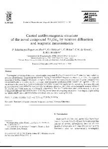
1.2.1 Background In this section, we consider the communications channel, which exists between the transmitter and the receiver, as shown in Figure 1.1. Accurate characterization of this channel is essential if we are to remove the impairments imposed by the channel using signal processing at the receiver. Here we initially consider only fixed communications links whereby both terminals are stationary, although mobile radio communications channels, which change significantly with time, are becoming more prevalent. We define fixed communications channels to be those between a fixed transmitter and a fixed receiver. These channels are exemplified by twisted pairs, cables, wave guides, optical fiber and point-to-point microwave radio channels. Whatever the nature of the channel, its output signal differs from the input signal. The difference might be deterministic or random, but it is typically unknown to the receiver. Examples of channel impairments are dispersion, nonlinear distortions, delay, and random noise. Fixed communications channels can often be modeled by a linear transfer function, which describes the channel dispersion. The ubiquitous additive Gaussian noise (AWGN) is a fundamental limiting factor in communications via linear time-invariant (LTI) channels. Although the channel characteristics might change due to factors such as aging, temperature changes, and channel switching, these variations will not be apparent over the course of a typical communication session. It is this inherent time invariance that characterizes fixed channels. An ideal, distortion-free communications channel would have a flat frequency response and linear phase response over the frequency range of −∞ . . . + ∞, although in practice it is sufficient to satisfy this condition over the bandwidth (B) of the signals to be transmitted, as seen in Figure 1.2. In this figure, A(ω) represents the magnitude of the channel response at frequency w, and φ(w) = wT represents the phase shift at frequency w due to the circuit delay T . Practical channels always have some linear distortions due to their bandlimited, nonflat frequency response and nonlinear phase response. In addition, the group-delay response of the channel, which is the derivative of the phase response, is often given. 1.2.2 Practical Gaussian Channels Conventional telephony uses twisted copper wire pairs to connect subscribers to the local exchange. The bandwidth is approximately 3.4 kHz, and the waveform distortions are relatively benign. For applications requiring a higher bandwidth, coaxial cables can be used. Their attenuation increases approximately with the square root of the frequency. Hence, for wideband, long-distance operation, they require channel equalization. Typically, coaxial cables can provide a bandwidth of about 50 MHz, and the transmission rate they can support is limited by the so-called skin effect. Point-to-point microwave radio channels typically utilize high-gain directional transmit and receive antennas in a line-of-sight scenario, where free-space propagation conditions may be applicable.

16

1.2.3. Gaussian Noise

Η(ω) ωΤ 1

Α(ω)

ω B Figure 1.2: Ideal, distortion-free channel model having a linear phase and a flat magnitude response. 1.2.3 Gaussian Noise Regardless of the communications channel used, random noise is always present. Noise can be broadly classified as natural or man-made. Examples of man-made noise are those due to electrical appliances, and fluorescent lighting, and the effects of these sources can usually be mitigated at the source. Natural noise sources affecting radio transmissions include galactic star radiations and atmospheric noise. There exists a low-noise frequency window in the range of 1–10 GHz, where the effects of these sources are minimized. Natural thermal noise is ubiquitous. This is due to the random motion of electrons, and it can be reduced by reducing the temperature. Since thermal noise contains practically all frequency components up to some 1013 Hz with equal power, it is often referred to as white noise (WN) in an analogy to white light containing all colors with equal intensity. This WN process can be characterized by its uniform power spectral density (PSD) N (ω) = N0 /2 shown together with its autocorrelation function (ACF) in Figure 1.3. The power spectral density of any signal can be conveniently measured by the help of a selective narrowband power meter tuned across the bandwidth of the signal. The power measured at any frequency is then plotted against the measurement frequency. The autocorrelation function R(τ ) of the signal x(t) gives an average indication of how predictable the signal x(t) is after a period of τ seconds from its present value. Accordingly, it is defined as follows: Z 1 ∞ x(t)x(t + τ )dt. (1.2) R(τ ) = lim T →∞ T −∞ For a periodic signal x(t), it is sufficient to evaluate the above equation for a single period T0 , yielding: Z T0 /2 1 x(t)x(t + τ )dt. (1.3) R(τ ) = T0 −T0 /2

1.2.3. Gaussian Noise

17

Figure 1.3: Power spectral density and autocorrelation of WN. The basic properties of the ACF are: • The ACF is symmetric: R(τ ) = R(−τ ). • The ACF is monotonously decreasing: R(τ ) ≤ R(0). • For τ = 0 we have R(0) = x2 (t), which is the signal’s power. • The ACF and the PSD form a Fourier transform pair, which is formally stated as the Wiener-Khintchine theorem, as follows:

R(τ )

= = =

1 2π

Z

∞

N (ω)ejωτ dω

−∞

Z ∞ 1 N0 ejωτ dω 2π −∞ 2 Z 1 N0 ∞ jωτ N0 δ(τ ), e dω = 2π 2 −∞ 2

(1.4)

where δ(τ ) is the Dirac delta function. Clearly, for any timed-domain shift τ > 0, the noise is uncorrelated. Bandlimited communications systems bandlimit not only the signal but the noise as well, and this filtering limits the rate of change of the time-domain noise signal, introducing some correlation over the interval of ±1/2B. The stylized PSD and ACF of bandlimited white noise are displayed in Figure 1.4.

18

1.3. Information of a Source

NB(f)

R( )=NoB.sinc(2 B )

No 2

1 2B

0

-B

B

f

0

Figure 1.4: Power spectral density and autocorrelation of bandlimited WN. After bandlimiting, the autocorrelation function becomes: R(τ )

= = = =

Z N0 B j2πf τ N0 jωτ e dω = e df 2 −B −B 2  B N0 ej2πf τ 2 j2πτ −B 1 [cos 2πBτ + j sin 2πBτ − cos 2πBτ + j sin 2πBτ ] j2πτ sin(2πBτ ) , N0 B 2πBτ 1 2π

Z

B

(1.5)

which is the well-known sinc-function seen in Figure 1.4. In the time-domain, the amplitude distribution of the white thermal noise has a normal or Gaussian distribution, and since it is inevitably added to the received signal, it is usually referred to as additive white Gaussian noise (AWGN). Note that AWGN is therefore the noise generated in the receiver. The probability density function (PDF) is the well-known bell-shaped curve of the Gaussian distribution, given by 2 1 p(x) = √ e−(x−m)/2σ , σ 2π

(1.6)

where m is the mean and σ 2 is the variance. The effects of AWGN can be mitigated by increasing the transmitted signal power and thereby reducing the relative effects of noise. The signal-to-noise ratio (SNR) at the receiver’s input provides a good measure of the received signal quality. This SNR is often referred to as the channel SNR.

1.3

Information of a Source

Based on Shannon’s work [24–27, 35, 36], let us introduce the basic terms and definitions of information theory by considering a few simple examples. Assume that a simple 8-bit

1.3. Information of a Source

19

analog-to-digital (ADC) converter emits a sequence of mutually independent source symbols that can take the values i = 1, 2, . . . 256 with equal probability. One may wonder, how much information can be inferred upon receiving one of these samples? It is intuitively clear that this inferred information is definitely proportional to the “uncertainty” resolved by the reception of one such symbol, which in turn implies that the information conveyed is related to the number of levels in the ADC. More explicitly, the higher the number of legitimate quantization levels, the lower the relative frequency or probability of receiving any one of them and hence the more “surprising,” when any one of them is received. Therefore, less probable quantized samples carry more information than their more frequent, more likely counterparts. Not suprisingly, one could resolve this uncertainty by simply asking a maximum of 256 questions, such as “Is the level 1?” “Is it 2? . . .” “Is it 256?” Following Hartley’s approach [29], a more efficient strategy would be to ask eight questions, such as: “Is the level larger than 128?” No. “Is it larger than 64?” No. . . . “Is it larger than 2?” No. “Is it larger than 1?” No. Clearly, the source symbol emitted was of magnitude one, provided that the zero level was not used. We could therefore infer that log2 256 = 8 “Yes/No” binary answers were needed to resolve any uncertainty as regards the source symbol’s level. In more general terms, the information carried by any one symbol of a q-level source, where all the levels are equiprobable with probabilities of pi = 1/q, i = 1 . . . q, is defined as I = log2 q. (1.7) Rewriting Equation 1.7 using the message probabilities pi = form: 1 I = log2 = −log2 pi , pi

1 q

yields a more convenient (1.8)

which now is also applicable in case of arbitrary, unequal message probabilities pi , again, implying the plausible fact that the lower the probability of a certain source symbol, the higher the information conveyed by its occurrence. Observe, however, that for unquantized analog sources, where as regards to the number of possible source symbols we have q → ∞ and hence the probability of any analog sample becomes infinitesimally low, these definitions become meaningless. Let us now consider a sequence of N consecutive q-ary symbols. This sequence can take q N number of different values, delivering q N different messages. Therefore, the information carried by one such sequence is: IN = log2 (q N ) = N log2 q,

(1.9)

which is in perfect harmony with our expectation, delivering N times the information of a single symbol, which was quantified by Equation 1.7. Doubling the sequence length to 2N carries twice the information, as suggested by: I2N = log2 (q 2N ) = 2N · log2 q.

(1.10)

Before we proceed, let us briefly summarize the basic properties of information following Shannon’s work [24–27, 35, 36]:

20

1.4. Average Information of Discrete Memoryless Sources • If for the probability of occurrences of the symbols j and k we have pj < pk , then as regards the information carried by them we have: I(k) < I(j). • If in the limit we have pk → 1, then for the information carried by the symbol k we have I(k) → 0, implying that symbols, whose probability of occurrence tends to unity, carry no information. • If the symbol probability is in the range of 0 ≤ pk ≤ 1, then as regards the information carried by it we have I(k) ≥ 0. • For independent messages k and j, their joint information is given by the sum of their information: I(k, j) = I(k) + I(j). For example, the information carried by the statement “My son is 14 years old and my daughter is 12” is equivalent to that of the sum of these statements: “My son is 14 years old” and “My daughter is 12 years old.” • In harmony with our expectation, if we have two equiprobable messages 0 and 1 with probabilities, p1 = p2 = 21 , then from Equation 1.8 we have I(0) = I(1) = 1 bit.

1.4 Average Information of Discrete Memoryless Sources Following Shannon’s approach [24–27, 35, 36], let us now consider a source emitting one of q possible symbols from the alphabet s = s1 , s2 , . . . si . . . sq having symbol probabilities of pi , i = 1, 2, . . . q. Suppose that a long message of N symbols constituted by symbols from the alphabet s = s1 , s2 , . . . sq having symbol probabilities of pi is to be transmitted. Then the symbol si appears in every N -symbol message on the average pi · N number of times, provided the message length is sufficiently long. The information carried by symbol si is log2 1/pi and its pi · N occurrences yield an information contribution of I(i) = pi · N · log2

1 . pi

(1.11)

Upon summing the contributions of all the q symbols, we acquire the total information carried by the N -symbol sequence: I=

q X i=1

pi N · log2

1 [bits]. pi

(1.12)

Averaging this over the N symbols of the sequence yields the average information per symbol, which is referred to as the source’s entropy [25] : q q X X 1 I pi log2 pi [bit/symbol]. pi · log2 = − = H= N pi i=1 i=1

(1.13)

Then the average source information rate can be defined as the product of the information carried by a source symbol, given by the entropy H and the source emission rate Rs : R = Rs · H [bits/sec].

(1.14)

1.4.1. Maximum Entropy of a Binary Source

21

Observe that Equation 1.13 is analogous to the discrete form of the first moment or in other words the mean of a random process with a probability density function (PDF) of p(x), as in Z ∞ x= x · p(x)dx, (1.15) −∞

where the averaging corresponds to the integration, and the instantaneous value of the random variable x represents the information log2 pi carried by message i, which is weighted by its probability of occurrence pi quantified for a continuous variable x by p(x). 1.4.1 Maximum Entropy of a Binary Source Let us assume that a binary source, for which q = 2, emits two symbols with probabilities p1 = p and p2 = (1 − p), where the sum of the symbol probabilities must be unity. In order to quantify the maximum average information of a symbol from this source as a function of the symbol probabilities, we note from Equation 1.13 that the entropy is given by: H(p) = −p · log2 p − (1 − p) · log2 (1 − p).

(1.16)

As in any maximization problem, we set ∂H(p)/∂p = 0, and upon using the differentiation chain rule of (u · v)′ = u′ · v + u · v ′ as well as exploiting that (loga x)′ = x1 loga e we arrive at: ∂H(p) ∂p log2 p

=

p p

= =

=

p (1 − p) · log2 e + log2 (1 − p) + log e = 0 p (1 − p) 2 log2 (1 − p) −log2 p − (1 − p) 0.5.

This result suggests that the entropy is maximum for equiprobable binary messages. Plotting Equation 1.16 for arbitrary p values yields Figure 1.5, in which Shannon suggested that the average information carried by a symbol of a binary source is low, if one of the symbols has a high probability, while the other a low probability. Example: Let us compute the entropy of the binary source having message probabilities of p1 = 81 , p2 = 87 . The entropy is expressed as: 1 1 7 7 H = − log2 − log2 . 8 8 8 8 Exploiting the following equivalence: log2 (x)

=

log10 (x) · log2 (10) ≈ 3.322 · log10 (x)

we have: H

≈

3 7 7 − · 3.322 · log10 ≈ 0.54 [bit/symbol], 8 8 8

(1.17)

1.4.2. Maximum Entropy of a q-ary Source

22

1.0

H(p)

0.8 0.6 0.4 0.2 0.0 0.0

0.1

0.2

0.3

0.4

0.5

p

0.6

0.7

0.8

0.9

1.0

c Figure 1.5: Entropy versus message probability p for a binary source. Shannon [25], BSTJ, 1948. again implying that if the symbol probabilities are rather different, the entropy becomes significantly lower than the achievable 1 bit/symbol. This is because the probability of encountering the more likely symbol is so close to unity that it carries hardly any information, which cannot be compensated by the more “informative” symbol’s reception. For the even more unbalanced situation of p1 = 0.1 and p2 = 0.9 we have: H

= −0.1 log2 0.1 − 0.9 · log2 0.9

≈ −(0.3322 · log10 0.1 + 0.9 · 3.322 · log10 0.9)

≈ 0.3322 + 0.1368 ≈ 0.47 [bit/symbol].

In the extreme case of p1 = 0 or p2 = 1 we have H = 0. As stated before, the average source information rate is defined as the product of the information carried by a source symbol, given by the entropy H and the source emission rate Rs , yielding R = Rs ·H [bits/sec]. Transmitting the source symbols via a perfect noiseless channel yields the same received sequence without loss of information. 1.4.2 Maximum Entropy of a q-ary Source For a q-ary source the entropy is given by: H=−

q X

pi log2 pi ,

(1.18)

i=1

P where, again, the constraint pi = 1 must be satisfied. When determining P the extreme value of the above expression for the entropy H under the constraint of pi = 1, the

1.5. Source Coding for a Discrete Memoryless Source

23

following term has to be maximized: D

=

q X i=1

"

−pi log2 pi + λ · 1 −

q X

#

pi ,

i=1

(1.19)

where λ is the so-called Lagrange multiplier. Following the standard procedure of maximizing an expression, we set: ∂D pi = − log2 pi − · log2 e − λ = 0 ∂pi pi leading to log2 pi = −(log2 e + λ) = Constant for i = 1 . . . q, which implies that the maximum entropy of a q-ary source is maintained, if all message probabilities are identical, although at this stage the value of this constant probability is not explicit. Note, however, that the message probabilites must sum to unity, and hence: q X i=1

pi = 1 = q · a,

(1.20)

where a is a constant, leading to a = 1/q = pi , implying that the entropy of any q-ary source is maximum for equiprobable messages. Furthermore, H is always bounded according to: 0 ≤ H ≤ log2 q.

(1.21)

1.5 Source Coding for a Discrete Memoryless Source Interpreting Shannon’s work [24–27, 35, 36] further, we see that source coding is the process by which the output of a q-ary information source is converted to a binary sequence for transmission via binary channels, as seen in Figure 1.1. When a discrete memoryless source generates q-ary equiprobable symbols with an average information rate of R = Rs log2 q, all symbols convey the same amount of information, and efficient signaling takes the form of binary transmissions at a rate of R bps. When the symbol probabilities are unequal, the minimum required source rate for distortionless transmission is reduced to R = Rs · H < Rs log2 q.

(1.22)

Then the transmission of a highly probable symbol carries little information and hence assigning log2 q number of bits to it does not use the channel efficiently. What can be done to improve transmission efficiency? Shannon’s source coding theorem suggests that by using a source encoder before transmission the efficiency of the system with equiprobable source symbols can be arbitrarily approached.

24

1.5.1. Shannon-Fano Coding

Algorithm 1 (Shannon-Fano Coding) This algorithm summarizes the Shannon-Fano coding steps. (See also Figure 1.6 and Table 1.1.) 1. The source symbols S0 . . . S7 are first sorted in descending order of probability of occurrence. 2. Then the symbols are divided into two subgroups so that the subgroup probabilities are as close to each other as possible. This is symbolized by the horizontal divisions in Table 1.1. 3. When allocating codewords to represent the source symbols, we assign a logical zero to the top subgroup and logical one to the bottom subgroup in the appropriate column under ‘‘coding steps.’’ 4. If there is more than one symbol in the subgroup, this method is continued until no further divisions are possible. 5. Finally, the variable-length codewords are output to the channel.

Coding efficiency can be defined as the ratio of the source information rate and the average output bit rate of the source encoder. If this ratio approaches unity, implying that the source encoder’s output rate is close to the source information rate, the source encoder is highly efficient. There are many source encoding algorithms, but the most powerful approach suggested was Shannon’s method [24], which is best illustrated by means of the following example, portrayed in Table 1.1, Algorithm 1, and Figure 1.6. 1.5.1 Shannon-Fano Coding The Shannon-Fano coding algorithm is based on the simple concept of encoding frequent messages using short codewords and infrequent ones by long codewords, while reducing the average message length. This algorithm is part of virtually all treatises dealing with information theory, such as, for example, Carlson’s work [31]. The formal coding steps listed in Algorithm 1 and in the flowchart of Figure 1.6 can be readily followed in the context of a simple example in Table 1.1. The average codeword length is given by weighting the length of any codeword by its probability, yielding: (0.27 + 0.2) · 2 + (0.17 + 0.16) · 3 + 2 · 0.06 · 4 + 2 · 0.04 · 4 ≈ 2.73 [bit].

1.5.1. Shannon-Fano Coding

25

Sort source symbols in descending order of probabilities

Derive subgroups of near-equal probabilities

Assign zero & one to top and bottom branches, respectively

Yes

More than one symbols are in subgroups ?

No Stop, output encoded symbols Figure 1.6: Shannon-Fano Coding Algorithm (see also Table 1.1 and Algorithm 1).

Symb.

Prob.

S0 S1 S2 S3 S4 S5 S6 S7

0.27 0.20 0.17 0.16 0.06 0.06 0.04 0.04

Coding Steps 1 2 3 4 0 0 0 1 1 0 0 1 0 1 1 1 0 0 1 1 0 1 1 1 1 0 1 1 1 1

Codeword 00 01 100 101 1100 1101 1110 1111

Table 1.1: Shannon-Fano Coding Example Based on Algorithm 1 and Figure 1.6

26

1.5.2. Huffman Coding

Algorithm 2 (Huffman Coding) This algorithm summarizes the Huffman coding steps. 1. Arrange the symbol probabilities pi in decreasing order and consider them as ‘‘leaf-nodes,’’ as suggested by Table 1.2. 2. While there is more than one node, merge the two nodes having the lowest probability and assign 0/1 to the upper/lower branches, respectively. 3. Read the assigned ‘‘transition bits’’ on the branches from top to bottom in order to derive the codewords.

The entropy of the source is: H

= = ≈

≈

−

X

pi log2 pi

(1.23)

i

−(log2 10)

X

pi log10 pi

i

−3.322 · [0.27 · log10 0.27 + 0.2 · log10 0.2 +0.17 · log10 0.17 + 0.16 · log10 0.16

+2 · 0.06 · log10 0.06 + 2 · 0.04 · log10 0.04]

2.691 [bit/symbol].

Since the average codeword length of 2.73 bit/symbol is very close to the entropy of 2.691 bit/symbol, a high coding efficiency is predicted, which can be computed as: E≈

2.691 ≈ 98.6 %. 2.73

The straightforward 3 bit/symbol binary coded decimal (BCD) assignment gives an efficiency of: 2.691 E≈ ≈ 89.69 %. 3 In summary, Shannon-Fano coding allowed us to create a set of uniquely invertible mappings to a set of codewords, which facilitate a more efficient transmission of the source symbols, than straightforward BCD representations would. This was possible with no coding impairment (i.e., losslessly). Having highlighted the philosophy of the Shannon-Fano noiseless or distortionless coding technique, let us now concentrate on the closely related Huffman coding principle. 1.5.2 Huffman Coding The Huffman Coding (HC) algorithm is best understood by referring to the flowchart of Figure 1.7 and to the formal coding description of Algorithm 2, while a simple practical example is portrayed in Table 1.2, which leads to the Huffman codes summarized in Table 1.3. Note that we used the same symbol probabilities as in our Shannon-Fano coding example,

1.5.2. Huffman Coding

Symb.

Prob.

S0 S1 S2 S3 S4 S5 S6 S7

0.27 0.20 0.17 0.16 0.06 0.06 0.04 0.04

Symb.

Prob.

S23 S0 S1 S4567

0.33 0.27 0.20 0.20

27

Step 1 & 2 Code Prob.

0 1 0 1

0.12 0.08

Step 5 & 6 Code Prob. 0 0.6 1 0 0.4 1

Step 3 & 4 Code Prob.

0 1 0 0 1 1

Group

Code

0.33

S0 S1 S23

0.20

S4567

0 1 00 01 10 11

Step 7 Code Prob. 0 1.0 1

Codeword 00 01 10 11

Table 1.2: Huffman Coding Example Based on Algorithm 2 and Figure 1.7 (for final code assignment see Table 1.3)

Symbol S0 S1 S2 S3 S4 S5 S6 S7

Probability 0.27 0.20 0.17 0.16 0.06 0.06 0.04 0.04

BCD 000 001 010 011 100 101 110 111

Huffman Code 01 10 000 001 1100 1101 1110 1111

Table 1.3: Huffman Coding Example Summary of Table 1.2

28

1.5.2. Huffman Coding

Arrange source symbols in descending order of probabilities

Merge two of the lowest prob. symbols into one subgroup

Assign zero & one to top and bottom branches, respectively

Yes

Is there more than one unmerged node ?

No Stop, read transition bits on the branches from top to bottom to generate codewords Figure 1.7: Huffman coding algorithm (see also Algorithm 2 and Table 1.2). but the Huffman algorithm leads to a different codeword assignment. Nonetheless, the code’s efficiency is identical to that of the Shannon-Fano algorithm. The symbol-merging procedure can also be conveniently viewed using the example of Figure 1.8, where the Huffman codewords are derived by reading the associated 1 and 0 symbols from the end of the tree backward, that is, toward the source symbols S0 . . . S7 . Again, these codewords are summarized in Table 1.3. In order to arrive at a fixed average channel bit rate, which is convenient in many communications systems, a long buffer might be needed, causing storage and delay problems. Observe from Table 1.3 that the Huffman coding algorithm gives codewords that can be uniquely decoded, which is a crucial prerequisite for its practical employment. This is because no codeword can be a prefix of any longer one. For example, for the following sequence

0.27

0.20

S1=0.20

0.20

0.17

S2=0.17

0.06

S5=0.06

0.06

S6=0.04

0.08

0.16

0.20

0.60

0.33

0.20

0.17

0.12

0.40

0.27

0.20

0.16

0.08

S4=0.06

0.33

0.20

0.17

0.16

S3=0.16

0.27

0.27

0.40 0 1

0 1

1.5.2. Huffman Coding

0.27

S0=0.27

0 1

0 1

0 1

0 1

0 1 S7=0.04 Figure 1.8: Tree-based Huffman coding example.

29

30

1.6. Entropy of Discrete Sources Exhibiting Memory

of codewords . . . , 00, 10, 010, 110, 1111, . . . the source sequence of . . . S0 , S1 , S2 , S3 , S8 . . . can be uniquely inferred from Table 1.3. In our discussions so far, we have assumed that the source symbols were completely independent of each other. Such a source is usually referred to as a memoryless source. By contrast, sources where the probability of a certain symbol also depends on what the previous symbol was are often termed sources exhibiting memory. These sources are typically bandlimited sample sequences, such as, for example, a set of correlated or “similar-magnitude” speech samples or adjacent video pixels. Let us now consider sources that exhibit memory.

1.6

Entropy of Discrete Sources Exhibiting Memory

Let us invoke Shannon’s approach [24–27,35,36] in order to illustrate sources with and without memory. Let us therefore consider an uncorrelated random white Gaussian noise (WGN) process, which was passed through a low-pass filter. The corresponding autocorrelation functions (ACF) and power spectral density (PSD) functions were portrayed in Figures 1.3 and 1.4. Observe in the figures that through low-pass filtering a WGN process introduces correlation by limiting the rate at which amplitude changes are possible, smoothing the amplitude of abrupt noise peaks. This example suggests that all bandlimited signals are correlated over a finite interval. Most analog source signals, such as speech and video, are inherently correlated, owing to physical restrictions imposed on the analog source. Hence all practical analog sources possess some grade of memory, a property that is also retained after sampling and quantization. An important feature of sources with memory is that they are predictable to a certain extent, hence, they can usually be more efficiently encoded than unpredictable sources having no memory. 1.6.1 Two-State Markov Model for Discrete Sources Exhibiting Memory Let us now introduce a simple analytically tractable model for treating sources that exhibit memory. Predictable sources that have memory can be conveniently modeled by Markov processes. A source having a memory of one symbol interval directly “remembers” only the previously emitted source symbol and depending on this previous symbol it emits one of its legitimate symbols with a certain probability, which depends explicitly on the state associated with this previous symbol. A one-symbol-memory model is often referred to as a first-order model. For example, if in a first-order model the previous symbol can take only two different values, we have two different states, and this simple two-state first-order Markov model is characterized by the state transition diagram of Figure 1.9. Previously, in the context of Shannon-Fano and Huffman coding of memoryless information sources, we used the notation of Si , i = 0, 1, . . . for the various symbols to be encoded. In this section, we are dealing with sources exhibiting memory and hence for the sake of distinction we use the symbol notation of Xi , i = 1, 2, . . .. If, for the sake of illustration, the previous emitted symbol was X1 , the state machine of Figure 1.9 is in state X1 , and in the current signaling interval it can generate one of two symbols, namely, X1 and X2 , whose probability depends explicitly on the previous state X1 . However, not all two-state Markov models are as simple as that of Figure 1.9, since the transitions from state X1 to X2 are not necessarily associated with emitting the same symbol as the transitions from state X2 to X1 . Thus more elaborate example will be considered later in this chapter.

1.6.2. N -State Markov Model for Discrete Sources Exhibiting Memory

31

Observe in Figure 1.9 that the corresponding transition probabilities from state X1 are given by the conditional probabilities p12 = P (X2 /X1 ) and p11 = P (X1 /X1 ) = 1 − P (X2 /X1 ). Similar findings can be observed as regards state X2 . These dependencies can also be stated from a different point of view as follows. The probability of occurrence of a particular symbol depends not only on the symbol itself, but also on the previous symbol emitted. Thus, the symbol entropy for state X1 and X2 will now be characterized by means of the conditional probabilities associated with the transitions merging in these states. Explicitly, the symbol entropy for state Xi , i = 1, 2 is given by: Hi

=

2 X j=1

=

pij · log2

pi1 · log2

1 i = 1, 2 pij

1 1 + pi2 · log2 , pi1 pi2

(1.24)

yielding the symbol entropies, that is, the average information carried by the symbols emitted in states X1 and X2 , respectively, as: H1

=

H2

=

1 1 + p12 · log2 p11 p12 1 1 + p22 · log2 . p21 · log2 p21 p22

p11 · log2

(1.25)

Both symbol entropies, H1 and H2 , are characteristic of the average information conveyed by a symbol emitted in state X1 and X2 , respectively. In order to compute the overall entropy H of this source, they must be weighted by the probability of occurrence, P1 and P2 , of these states: H

= =

2 X

i=1 2 X i=1

Pi Hi Pi

2 X j=1

pij log2

1 . pij

(1.26)

Assuming a highly predictable source having high adjacent sample correlation, it is plausible that once the source is in a given state, it is more likely to remain in that state than to traverse into the other state. For example, assuming that the state machine of Figure 1.9 is in state X1 and the source is a highly correlated, predictable source, we are likely to observe long runs of X1 . Conversely, once in state X2 , long strings of X2 symbols will typically follow. 1.6.2 N -State Markov Model for Discrete Sources Exhibiting Memory In general, assuming N legitimate states, (i.e., N possible source symbols) and following similar arguments, Markov models are characterised by their state probabilities P (Xi ), i = 1 . . . N , where N is the number of states, as well as by the transition probabilities pij = P (Xi /Xj ),

1.6.2. N -State Markov Model for Discrete Sources Exhibiting Memory

32

'  - 6 &

$ ?      %

p12 = P (X2 =X1 )

P (X1 )

P (X2)

X1

p11

=

X2

p21 = P (X1 =X2 )

P (X1=X1 ) = 1 ? P (X2 =X1) p22

=1

? P (X1=X2 ) = P (X2=X2 )

Figure 1.9: Two-state first-order Markov model. where pij explicitly indicates the probability of traversing from state Xj to state Xi . Their further basic feature is that they emit a source symbol at every state transition, as will be shown in the context of an example presented in Section 1.7. Similarly to the two-state model, we define the entropy of a source having memory as the weighted average of the entropy of the individual symbols emitted from each state, where weighting is carried out taking into account the probability of occurrence of the individual states, namely Pi . In analytical terms , the symbol entropy for state Xi , i = 1 . . . N is given by: Hi =

N X j=1

pij · log2

1 i = 1 . . . N. pij

(1.27)

The averaged, weighted symbol entropies give the source entropy: H

=

N X

Pi Hi

i=1

=

N X i=1

Pi

N X

pij log2

j=1

1 . pij

(1.28)

Finally, assuming a source symbol rate of vs , the average information emission rate R of the source is given by: R = vs · H [bps].

(1.29)

1.7. Examples

a

33

'  - 6 &

p12 =0.1

X1

$ ?      % X2

0.9

b

0.1

p21 =0.9

P1 = 0:8

P2 = 0:2

d

Figure 1.10: Two-state Markov model example.

1.7

Examples

1.7.1 Two-State Markov Model Example As mentioned in the previous section, we now consider a slightly more sophisticated Markov model, where the symbols emitted upon traversing from state X1 to X2 are different from those when traversing from state X2 to X1 . More explicitly: • Consider a discrete source that was described by the two-state Markov model of Figure 1.9, where the transition probabilities are p11 = P (X1 /X1 ) = 0.9

p22 = P (X2 /X2 ) = 0.1

p12 = P (X1 /X2 ) = 0.1 p21 = P (X2 /X1 ) = 0.9, while the state probabilities are P (X1 ) = 0.8 and P (X2 ) = 0.2.

(1.30)

The source emits one of four symbols, namely, a, b, c, and d, upon every state transition, as seen in Figure 1.10. Let us find (a) the source entropy and (b) the average information content per symbol in messages of one, two, and three symbols. • Message Probabilities Let us consider two sample sequences acb and aab. As shown in Figure 1.10, the transitions leading to acb are (1 ; 1), (1 ; 2), and (2 ; 2). The probability of encountering this sequence is 0.8 · 0.9 · 0.1 · 0.1 = 0.0072. The sequence aab has a probability of zero because the transition from a to b is illegal. Further path (i.e., message) probabilities are tabulated in Table 1.4 along with the information of I = − log2 P of all the legitimate messages.

34

1.7.1. Two-State Markov Model Example Message Probabilities Pa = 0.9 × 0.8 = 0.72 Pb = 0.1 × 0.2 = 0.02 Pc = 0.1 × 0.8 = 0.08 Pd = 0.9 × 0.2 = 0.18 Paa = 0.72 × 0.9 = 0.648 Pac = 0.72 × 0.1 = 0.072 Pcb = 0.08 × 0.1 = 0.008 Pcd = 0.08 × 0.9 = 0.072 Pbb = 0.02 × 0.1 = 0.002 Pbd = 0.02 × 0.9 = 0.018 Pda = 0.18 × 0.9 = 0.162 Pdc = 0.18 × 0.1 = 0.018

Information conveyed (bit/message) Ia = 0.474 Ib = 5.644 Ic = 3.644 Id = 2.474 Iaa = 0.626 Iac = 3.796 Icb = 6.966 Icd = 3.796 Ibb = 8.966 Ibd = 5.796 Ida = 2.626 Idc = 5.796

Table 1.4: Message Probabilities of Example • Source Entropy – According to Equation 1.27, the entropy of symbols X1 and X2 is computed as follows: H1

= =

H2

≈ = ≈

−p12 · log2 p12 − p11 · log2 p11 1 0.1 · log2 10 + 0.9 · log2 0.9 0.469 bit/symbol −p21 · log2 p21 − p22 · log2 p22 0.469 bit/symbol

(1.31) (1.32)

– Then their weighted average is calculated using the probability of occurrence of each state in order to derive the average information per message for this source: H ≈ 0.8 · 0.469 + 0.2 · 0.469 ≈ 0.469 bit/symbol. – The average information per symbol I2 in two-symbol messages is computed from the entropy h2 of the two-symbol messages as follows: h2

=

8 X 1

Psymbol · Isymbol

= Paa · Iaa + Pac · Iac + . . . + Pdc · Idc ≈ 1.66 bits/2 symbols,

(1.33)

giving I2 = h2 /2 ≈ 0.83 bits/symbol information on average upon receiving a two-symbol message.

1.7.2. Four-State Markov Model for a 2-Bit Quantizer

35

– There are eight two-symbol messages; hence, the maximum possible information conveyed is log2 8 = 3 bits/2 symbols, or 1.5 bits/symbol. However, since the symbol probabilities of P1 = 0.8 and P2 = 0.2 are fairly different, this scheme has a significantly lower conveyed information per symbol, namely, I2 ≈ 0.83 bits/symbol. – Similarly, one can find the average information content per symbol for arbitrarily long messages of concatenated source symbols. For one-symbol messages we have: I1 = h1

=

4 X 1

= ≈

≈ ≈

Psymbol · Isymbol

Pa · Ia + . . . + Pd · Id 0.72 × 0.474 + . . . + 0.18 × 2.474

0.341 + 0.113 + 0.292 + 0.445 1.191 bit/symbol.

(1.34)

We note that the maximum possible information carried by one-symbol messages is h1max = log2 4 = 2 bit/symbol, since there are four one-symbol messages in Table 1.4. • Observe the important tendency, in which, when sending longer messages of dependent sources, the average information content per symbol is reduced. This is due to the source’s memory, since consecutive symbol emissions are dependent on previous ones and hence do not carry as much information as independent source symbols. This becomes explicit by comparing I1 ≈ 1.191 and I2 ≈ 0.83 bits/symbol. • Therefore, expanding the message length to be encoded yields more efficient coding schemes, requiring a lower number of bits, if the source has a memory. This is the essence of Shannon’s source coding theorem. 1.7.2 Four-State Markov Model for a 2-Bit Quantizer Let us now augment the previously introduced two-state Markov-model concepts with the aid of a four-state example. Let us assume that we have a discrete source constituted by a 2-bit quantizer, which is characterized by Figure 1.11. Assume further that due to bandlimitation only transitions to adjacent quantization intervals are possible, since the bandlimitation restricts the input signal’s rate of change. The probability of the signal samples residing in intervals 1–4 is given by: P (1) = P (4) = 0.1,

P (2) = P (3) = 0.4.

The associated state transition probabilities are shown in Figure 1.11, along with the quantized samples a, b, c, and d, which are transmitted when a state transition takes place, that is, when taking a new sample from the analog source signal at the sampling-rate fs . Although we have stipulated a number of simplifying assumptions, this example attempts to illustrate the construction of Markov models in the context of a simple practical problem.

36

1.8. Generating Model Sources

P(2)=0.4

b

p =0.8 12

p =0.2 11

a

1

2

b

p =0.4 22

a

P(1)=0.1

p =0.2 21

p =0.4

b

c

p =0.4

32

23

c

p =0.8 p =0.2 44

d

43

4

3

c

p =0.4 33

d

p(4)=0.1

p =0.2 34

P(3)=0.4

Figure 1.11: Four-state Markov model for a 2-bit quantizer. Next we construct a simpler example for augmenting the underlying concepts and set aside the above four-state Markov-model example as a potential exercise for the reader.

1.8

Generating Model Sources

1.8.1 Autoregressive Model In evaluating the performance of information processing systems, such as encoders and predictors, it is necessary to have “standardized” or easily described model sources. Although a set of semistandardized speech and images test sequences is widely used by researchers in codec performance testing, in contrast to analytical model sources, real speech or image sources cannot be used in analytical studies. A widely used analytical model source is the Autoregressive (AR) model. A zero mean random sequence y(n) is called an AR process of order p, if it is generated as follows: y(n) =

p X

k=1

ak y(n − k) + ε(n), ∀n,

(1.35)

1.8.2. AR Model Properties

37

where ε(n) is an uncorrelated zero-mean, random input sequence with variance σ 2 ; that is, E{ε(n)} = 0 E{ε2 (n)} = σ 2 E{ε(n) · y(m)} = 0.

(1.36)

From Equation 1.35 we surmise that an AR system recursively generates the present output from p number of previous output samples given by y(n − k) and the present random input sample ε(n). 1.8.2 AR Model Properties AR models are very useful in studying information processing systems, such as speech and image codecs, predictors, and quantizers. They have the following basic properties: 1. The first term of Equation 1.35, which is repeated here for convenience, yˆ(n) =

p X

k=1

ak y(n − k)

defines a predictor, giving an estimate yˆ(n) of y(n), which is associated with the minimum mean squared error between the two quantities. 2. Although yˆ(n) and y(n) depend explicitly only on the past p number of samples of y(n), through the recursive relationship of Equation 1.35 this entails the entire past of y(n). This is because each of the previous p samples depends on their predecessors. 3. Then Equation 1.35 can be written in the form of: y(n) = yˆ(n) + ε(n),

(1.37)

where ε(n) is the prediction error and yˆ(n) is the minimum variance prediction estimate of y(n). 4. Without proof, we state that for a random Gaussian distributed prediction error sequence ε(n) these properties are characteristic of a pth order Markov process portrayed in Figure 1.12. When this model is simplified for the case of p = 1, we arrive at the schematic diagram shown in Figure 1.13. 5. The power spectral density (PSD) of the prediction error sequence ε(n) is that of a random “white-noise” sequence, containing all possible frequency components with the same energy. Hence, its autocorrelation function (ACF) is the Kronecker delta function, given by the Wiener-Khintchine theorem: E{ε(n) · ε(m)} = σ 2 δ(n − m).

(1.38)

1.8.3 First-Order Markov Model A variety of practical information sources are adequately modeled by the analytically tractable first-order Markov model depicted in Figure 1.13, where the prediction order is p = 1. With

38

1.8.3. First-Order Markov Model

ε(n) - +

y(n) -

6

y(n − p)

y(n − 1) ···

T

T

T

T



a2 a1   × ×

ap ×  ?

?

P

?

Figure 1.12: Markov model of order p. ε(n) - +

y(n) -

6 T ?ap ×  Figure 1.13: First-order Markov model. the aid of Equation 1.35 we have y(n) = ε(n) + ay(n − 1), where a is the adjacent sample correlation of the process y(n). Using the following recursion: y(n − 1) = ε(n − 1) + a1 y(n − 2) .. .. .. . . . y(n − k) = ε(n − k) + a1 y(n − k − 1)

(1.39)

1.9. Run-Length Coding for Discrete Sources Exhibiting Memory

39

Predictor  Q-ary Source

x ˆ(i) Q-ary to x(i) ? - Binary - + e(i) Conv.

-

RL Encoder

-

Predictor  Q-ary  Output

x ˆ(i) Binary ? to Q-ary  +  e(i) Conv. x(i)

RL  Decoder

c Figure 1.14: Predictive run-length codec scheme. Carlson [31]. we arrive at: y(n) = =

ε(n) + a1 [ε(n − 1) + ay(n − 2)] ε(n) + a1 ε(n − 1) + a2 y(n − 2),

which can be generalized to: y(n) =

∞ X j=0

aj ε(n − j).

(1.40)

Clearly, Equation 1.40 describes the first-order Markov process by the help of the adjacent sample correlation a1 and the uncorrelated zero-mean random Gaussian process ε(n).

1.9

Run-Length Coding for Discrete Sources Exhibiting Memory

1.9.1 Run-Length Coding Principle [31] For discrete sources having memory, (i.e., possessing intersample correlation), the coding efficiency can be significantly improved by predictive coding, allowing the required transmission rate and hence the channel bandwidth to be reduced. Particularly amenable to run-length coding are binary sources with inherent memory, such as black and white documents, where the predominance of white pixels suggests that a Run-Length-Coding (RLC) scheme, which encodes the length of zero runs, rather than repeating long strings of zeros, provides high coding efficiency. Following Carlson’s interpretation [31], a predictive RLC scheme can be constructed according to Figure 1.14. The q-ary source messages are first converted to binary bit format.

40

1.9.2. Run-Length Coding Compression Ratio Length of 0-run l 0 1 2 3 .. .

Encoder Output (n-bit codeword) 00 · · · 000 00 · · · 001 00 · · · 010 00 · · · 011 .. .

Decoder Output

N −1 ≥ N = 2n − 1

11 · · · 110 11 · · · 111

00 · · · 01 00 · · · 00

1 01 001 0001 .. .

c Carlson, 1975 [31] Table 1.5: Run-length Coding Table For example, if an 8-bit analog-digital converter (ADC) is used, the 8-bit digital samples are converted to binary format. This bit-stream, x(i), is then compared with the output signal of the predictor, xˆ(i), which is fed with the prediction error signal e(i). The comparator is a simple mod-2 gate, outputting a logical 1, whenever the prediction fails; that is, the predictor’s output is different from the incoming bit x(i). If, however, x(i) = x ˆ(i), the comparator indicates this by outputting a logical 0. For highly correlated signals from sources with significant memory the predictions are usually correct, and hence long strings of 0 runs are emitted, interspersed with an occasional 1. Thus, the prediction error signal e(i) can be efficiently run-length encoded by noting and transmitting the length of zero runs. The corresponding binary run-length coding principle becomes explicit from Table 1.5 and from our forthcoming coding efficiency analysis. 1.9.2 Run-Length Coding Compression Ratio [37] Following Jain’s interpretation [37], let us now investigate the RLC efficiency by assuming that a run of r successive logical 0s is followed by a 1. Instead of directly transmitting these strings, we represent such a string as an n-bit word giving the length of the 0-run between successive logical ones. When a 0-run longer than N = 2n − 1 bits occurs, this is signaled as the all 1 codeword, informing the decoder to wait for the next RLC codeword before releasing the decoded sequence. Again, the scheme’s operation is characterized by Table 1.5. Clearly, data compression is achieved if the average number of 0 data bits per run d is higher than the number of bits, n, required to encode the 0-run length. Let us therefore compute the average number of bits per run without RLC. If a run of r logical zeros are followed by a 1, the runlength is (r + 1). The expected or mean value of (r + 1), namely, d = (r + 1), is calculated by weighting each specific (r + 1) with its probability of occurrence that is, with its discrete PDF c(r) and then averaging the weighted components, in: d = (r + 1) =

N −1 X r=0

(r + 1) · c(r) + N c(N ).

(1.41)

1.9.2. Run-Length Coding Compression Ratio 0.9

$RCSfile: gofl.gle,v $

p=0.1 p=0.9

CDF of g( )

g( ) = p (1-p)

0.8 0.7 0.6 0.5 0.4 0.3 0.2 0.1 0.0

0

2

4

6

8

10

12

14

1.0 0.9 0.8 0.7 0.6 0.5 0.4 0.3 0.2 0.1 0.0

41 $RCSfile: cdfgofl.gle,v $

p=0.1 p=0.9

0

2

4

6

8

10

12

14

Figure 1.15: CDF and PDF of the geometric distribution of run-length l. The PDF of a run of r zeros followed by a 1 is given by:  r p (1 − p) 0 ≤ r ≤ N − 1 c(r) = pN r = N,

(1.42)

since the probability of N consecutive zeros is pN if r = N , while for shorter runs the joint probability of r zeros followed by a 1 is given by pr · (1 − p). The PDF and CDF of this distribution are shown in Figure 1.15 for p = 0.9 and p = 0.1, where p represents the probability of a logical zero bit. Substituting Equation 1.42 in Equation 1.41 gives: d = = = =

N · pN +

N −1 X r=0

(r + 1) · pr · (1 − p)

N · pN + 1 · p0 · (1 − p) + 2 · p · (1 − p) + . . . + N · pN −1 · (1 − p) N · pN + 1 + 2p + 3p2 + . . . + N · pN −1 − p − 2p2 . . . − N · pN 1 + p + p2 + · · · pN −1 .

(1.43)

Equation 1.43 is a simple geometric progression, given in closed form as: d=

1 − pN . 1−p

(1.44)

RLC Example: Using a run-length coding memory of M = 31 and a zero symbol probability of p = 0.95, characterize the RLC efficiency. Substituting N and p into Equation 1.44 for the average run-length we have: d=

1 − 0.204 1 − 0.9531 ≈ ≈ 15.92. 1 − 0.95 0.05

(1.45)

42

1.10. Information Transmission via Discrete Channels The compression ratio C achieved by RLC is given by: C=

d 1 − pN 15.92 = ≈ ≈ 3.18. n n(1 − p) 5

(1.46)

The achieved average bit rate is B=

n ≈ 0.314 bit/pixel, d

and the coding efficiency is computed as the ratio of the entropy (i.e., the lowest possible bit rate and the actual bit rate). The source entropy is given by: H

≈ −0.95 · 3.322 · log10 0.95 − 0.05 · 3.322 · log10 0.05 ≈ 0.286 bit/symbol,

(1.47)

giving a coding efficiency of: E = H/B ≈ 0.286/0.314 ≈ 91%. This concludes our RLC example.

1.10 Information Transmission via Discrete Channels Let us now return to Shannon’s classic references [24–27, 35, 36] and assume that both the channel and the source are discrete, and let us evaluate the amount of information transmitted via the channel. We define the channel capacity characterizing the channel and show that according to Shannon nearly error-free information transmission is possible at rates below the channel capacity via the binary symmetric channel (BSC). Let us begin our discourse with a simple introductory example. 1.10.1 Binary Symmetric Channel Example Let us assume that a binary source is emitting a logical 1 with a probability of P (1) = 0.7 and a logical 0 with a probability of P (0) = 0.3. The channel’s error probability is pe = 0.02. This scenario is characterized by the binary symmetric channel (BSC) model of Figure 1.16. The probability of error-free reception is given by that of receiving 1, when a logical 1 is transmitted plus the probability of receiving a 0 when 0 is transmitted, which is also plausible from Figure 1.16. For example, the first of these two component probabilities can be computed with the aid of Figure 1.16 as the product of the probability P (1) of a logical 1 being transmitted and the conditional probability P (1/1) of receiving a 1, given the condition that a 1 was transmitted: P (Y1 , X1 ) = P (X1 ) · P (Y1 /X1 ) P (1, 1) = P (1) · P (1/1) = 0.7 · 0.98 = 0.686.

(1.48)

1.10.1. Binary Symmetric Channel Example

P (1) = 0.7

1 − pe =0.98

1

43

3

1

pe =0.02

P (0) = 0.3

TX pe =0.02 1 − pe =0.98 0

RX s

0

c Figure 1.16: The binary symmetric channel. Shannon [26], BSTJ, 1948. Similarly, the probability of the error-free reception of a logical 0 is given by: P (Y0 , X0 ) = P (0, 0) =

P (X0 ) · P (Y0 /X0 )

P (0) · P (0/0) = 0.3 · 0.98 = 0.294,

giving the total probability of error-free reception as: Pcorrect = P (1, 1) + P (0, 0) = 0.98. Following similar arguments, the probability of erroneous reception is also given by two components. For example, using Figure 1.16, the probability of receiving a 1 when a 0 was transmitted is computed by multiplying the probability P (0) of a logical 0 being transmitted by the conditional probability P (1/0) of receiving a logical 1, given the fact that a 0 is known to have been transmitted: P (Y1 , X0 ) = P (1, 0) =

P (X0 ) · P (Y1 /X0 ) P (0) · P (1/0) = 0.3 · 0.02 = 0.006.

P (Y0 , X1 ) = P (0, 1) =

P (X1 ) · P (Y0 /X1 ) P (1) · P (0/1) = 0.7 · 0.02 = 0.014,

Conversely,

yielding a total error probability of: Perror = P (1, 0) + P (0, 1) = 0.02, which is constituted by the above two possible error events.

44

1.10.2. Bayes’ Rule

Viewing events from a different angle, we observe that the total probability of receiving 1 is that of receiving a transmitted 1 correctly plus a transmitted 0 incorrectly: P1

= =

P (1) · (1 − pe ) + P (0) · pe

(1.49)

0.7 · 0.98 + 0.3 · 0.02 = 0.686 + 0.006 = 0.692.

On the same note, the probability of receiving 0 is that of receiving a transmitted 0 correctly plus a transmitted 1 incorrectly: P0

= =

P (0) · (1 − pe ) + P (1) · pe 0.3 · 0.98 + 0.7 · 0.02 = 0.294 + 0.014 = 0.308.

(1.50)

In the next example, we further study the performance of the BSC for a range of different parameters in order to gain a deeper insight into its behavior. Example: Repeat the above calculations for P (1) = 1, 0.9, 0.5, and pe = 0, 0.1, 0.2, 0.5 using the BSC model of Figure 1.16. Compute and tabulate the probabilities P (1, 1), P (0, 0), P (1, 0), P (0, 1), Pcorrect , Perror , P1 , and P0 for these parameter combinations, including also their values for the previous example, namely, for P (1) = 0.7, P (0) = 0.3 and pe = 0.02. Here we neglected the details of the calculations and summarized the results in Table 1.6. Some of the above quantities are plotted for further study in Figure 1.17, which reveals the interdependency of the various probabilities for the interested reader. Having studied the performance of the BSC, the next question that arises is, how much information can be inferred upon reception of a 1 and a 0 over an imperfect (i.e., error-prone) channel. In order to answer this question, let us first generalize the above intuitive findings in the form of Bayes’ rule. 1.10.2 Bayes’ Rule Let Yj represent the received symbols and Xi the transmitted symbols having probabilities of P (Yj ) and P (Xi ), respectively. Let us also characterize the forward transition probabilities of the binary symmetric channel as suggested by Figure 1.18. Then in general, following from the previous introductory example, the joint probability P (Yj , Xi ) of receiving Yj , when the transmitted source symbol was Xi , is computed as the probability P (Xi ) of transmitting Xi , multiplied by the conditional probability P (Yj /Xi ) of receiving Yj , when Xi is known to have been transmitted: P (Yj , Xi ) =

P (Xi ) · P (Yj /Xi ),

(1.51)

a result that we have already intuitively exploited in the previous example. Since for the joint probabilities P (Yj , Xi ) = P (Xi , Yj ) holds, we have: P (Xi , Yj ) = =

P (Yj ) · P (Xi /Yj )

P (Xi ) · P (Yj /Xi ).

(1.52)

0 Table 1.6: BSC Performance Table

0.02

0.1

0.2

0.5

P (1)

P (0)

1 0.9 0.7 0.5 1 0.9 0.7 0.5 1 0.9 0.7 0.5 1 0.9 0.7 0.5 1 0.9 0.7 0.5

0 0.1 0.3 0.5 0 0.1 0.3 0.5 0 0.1 0.3 0.5 0 0.1 0.3 0.5 0 0.1 0.3 0.5

(1 − pe ) = P (1/1) = P (0/0) 1 1 1 1 0.98 0.98 0.98 0.98 0.9 0.9 0.9 0.9 0.8 0.8 0.8 0.8 0.5 0.5 0.5 0.5

P (1, 1)

P (0, 0)

1 0.9 0.7 0.5 0.98 0.882 0.686 0.49 0.9 0.81 0.63 0.45 0.8 0.72 0.56 0.40 0.5 0.45 0.35 0.25

0 0.1 0.3 0.5 0 0.098 0.294 0.49 0 0.09 0.27 0.45 0 0.08 0.24 0.40 0 0.05 0.15 0.25

pe = P (1/0) = P (0/1) 0 0 0 0 0.02 0.02 0.02 0.02 0.1 0.1 0.1 0.1 0.2 0.2 0.2 0.2 0.5 0.5 0.5 0.5

P (1, 0)

P (0, 1)

P1

P0

0 0 0 0 0 0.002 0.006 0.01 0 0.01 0.03 0.05 0 0.02 0.06 0.1 0 0.05 0.15 0.25

0 0 0 0 0.02 0.018 0.014 0.01 0.1 0.09 0.07 0.05 0.2 0.18 0.14 0.1 0.5 0.45 0.35 0.25

1 0.9 0.7 0.5 0.98 0.884 0.692 0.491 0.9 0.811 0.723 0.455 0.8 0.722 0.566 0.5 0.5 0.5 0.5 0.5

0 0.1 0.3 0.5 0.02 0.116 0.308 0.509 0.1 0.189 0.277 0.545 0.2 0.278 0.434 0.5 0.5 0.5 0.5 0.5

1.10.2. Bayes’ Rule

pe

45

46

1.10.2. Bayes’ Rule

1.0

0.75

0.75

0.5

pe=0 pe=0.125 pe=0.25 pe=0.375 pe=0.5

0.25

0.0 0.0

P(0,0)

P(1,1)

$RCSfile: bsc-performance.gle,v $

1.0

0.25

0.5

pe=0 pe=0.125 pe=0.25 pe=0.375 pe=0.5

0.5

0.25

0.75

0.0 0.0

1.0

0.25

1.0

1.0

0.75

0.75

0.5

pe=0.5 pe=0.375 pe=0.25 pe=0.125

0.25

0.0 0.0

0.25

0.5

0.5

0.75

1.0

0.75

1.0

P(0)

P(1,0)

P(0,1)

P(1)

0.5

pe=0.5 pe=0.375 pe=0.25 pe=0.125

0.25

0.75

1.0

0.0 0.0

P(1)

0.25

0.5

P(0)

Figure 1.17: BSC performance for pe = 0, 0.125, 0.25, 0.375, and 0.5.

P (Y0 /X0 ) X0

- Y 3 0

P (Y1 /X0 )

P (Y0 /X1 ) - Y1 s

X1 P (Y1 /X1 )

Figure 1.18: Forward transition probabilities of the nonideal binary symmetric channel.

1.10.3. Mutual Information

47

Equation 1.52 is often presented in the form: P (Xi /Yj ) = =

P (Xi , Yj ) P (Yj ) P (Yj ) · P (Xi /Yj ) , P (Yj )

(1.53)

which is referred to as Bayes’ rule. Logically, the probability of receiving a particular Yj = Yj0 is the sum of all joint probabilities P (Xi , Yj0 ) over the range of Xi . This corresponds to the probability of receiving the transmitted Xi correctly, giving rise to the channel output Yj0 plus the sum of the probabilities of all other possible transmitted symbols giving rise to Yj0 : X X P (Yj ) = P (Xi , Yj ) = P (Xi )P (Yj /Xi ). (1.54) X

X

Similarly: P (Xi )

=

X Y

P (Xi , Yj ) =

X

P (Yj )P (Xi /Yj ).

(1.55)

Y

1.10.3 Mutual Information In this section, we elaborate further on the ramifications of Shannon’s information theory [24– 27, 35, 36]. Over nonideal channels impairments are introduced, and the received information might be different from the transmitted information. In this section, we quantify the amount of information that can be inferred from the received symbols over noisy channels. In the spirit of Shannon’s fundamental work [24] and Carlson’s classic reference [31], let us continue our discourse with the definition of mutual information. We have already used the notation P (Xi ) to denote the probability that the source symbol Xi was transmitted and P (Yi ) to denote the probability that the symbol Yj was received. The joint probability that Xi was transmitted and Yj was received had been quantified by P (Xi , Yj ), and P (Xi /Yj ) indicated the conditional probability that Xi was transmitted, given that Yj was received, while P (Yj /Xi ) was used for the conditional probability that Yj was received given that Xi was transmitted. In case of i = j, the conditional probabilities P (Yj /Xj )j = 1 · · · q represent the errorfree transmission probabilities of the source symbols j = 1 · · · q. For example, in Figure 1.18 the probabilities P (Y0 /X0 ) and P (Y1 /X1 ) are the probabilities of the error-free reception of a transmitted X0 and X1 source symbol, respectively. The probabilities P (Yj /Xi )j 6= i, on the other hand, give the individual error probabilities, which are characteristic of error events that corrupted a transmitted symbol Xi to a received symbol of Yj . The corresponding error probabilities in Figure 1.18 are P (Y0 /X1 ) and P (Y1 /X0 ). Let us define the mutual information of Xi and Yj as: I(Xi , Yj ) = log2

P (Xi , Yj ) P (Yj /Xi ) P (Xi /Yj ) = log2 = log2 bits, P (Xi ) P (Xi ) · P (Yj ) P (Yj )

(1.56)

48

1.10.4. Mutual Information Example

which quantifies the amount of information conveyed, when Xi is transmitted and Yj is received. Over a perfect, noiseless channel, each received symbol Yj uniquely identifies a transmitted symbol Xi with a probability of P (Xi /Yj ) = 1. Substituting this probability in Equation 1.56 yields a mutual information of: I(Xi , Yj ) = log2

1 , P (Xi )

(1.57)

which is identical to the self-information of Xi and hence no information is lost over the channel. If the channel is very noisy and the error probability becomes 0.5, then the received symbol Yj becomes unrelated to the transmitted symbol Xi , since for a binary system upon its reception there is a probability of 0.5 that X0 was transmitted and the probability of X1 is also 0.5. Then formally Xi and Yj are independent and hence P (Xi /Yj ) =

P (Xi , Yj ) P (Xi ) · P (Yj ) = = P (Xi ), P (Yj ) P (Yj )

(1.58)

giving a mutual information of: I(Xi , Yj )

= log2

P (Xi ) = log2 1 = 0, P (Xi )

(1.59)

implying that no information is conveyed via the channel. Practical communications channels perform between these extreme values and are usually characterized by the average mutual information defined as: X I(X, Y ) = P (Xi , Yj ) · I(Xi , Yj ) x,y

=

X x,y

P (Xi , Yj ) · log2

P (Xi /Yj ) [bit/symbol]. P (Xi )

(1.60)

Clearly, the average mutual information in Equation 1.60 is computed by weighting each component I(Xi , Yj ) by its probability of occurrence P (Xi , Yj ) and summing these contributions for all combinations of Xi and Yj . The average mutual information I(X, Y ) defined above gives the average amount of source information acquired per received symbol, as distinguished from that per source symbol, which was given by the entropy H(X). Let us now consolidate these definitions by working through the following numerical example. 1.10.4 Mutual Information Example Using the same numeric values as in our introductory example as regards to the binary symmetric channel in Section 1.10.1, and exploiting that from Bayes’ rule in Equation 1.53, we have: P (Xi , Yj ) . P (Xi /Yj ) = P (Yj )

1.10.4. Mutual Information Example

49

The following probabilities can be derived, which will be used at a later stage, in order to determine the mutual information: P (X1 /Y1 ) = P (1/1) = and P (X0 /Y0 ) = P (0/0) =

P (1, 1) 0.686 = ≈ 0.9913 P1 0.692 0.294 P (0, 0) = ≈ 0.9545, P0 0.3080

where P1 = 0.692 and P0 = 0.3080 represent the total probability of receiving 1 and 0, respectively, which is the union of the respective events of error-free and erroneous receptions yielding the specific logical value concerned. The mutual information from Equation 1.56 is computed as: I(X1 , Y1 )

I(X0 , Y0 )

P (X1 /Y1 ) P (X1 ) 0.9913 ≈ 0.502 bit ≈ log2 0.7 0.9545 ≈ log2 ≈ 1.67 bit. 0.3 = log2

(1.61) (1.62)

These figures must be contrasted with the amount of source information conveyed by the source symbols X0 , X1 : I(0) = log2 and

1 ≈ log2 3.33 ≈ 1.737 bit/symbol 0.3

(1.63)

1 ≈ log2 1.43 ≈ 0.5146 bit/symbol. (1.64) 0.7 The amount of information “lost” in the noisy channel is given by the difference between the amount of information carried by the source symbols and the mutual information gained upon inferring a particular symbol at the noisy channel’s output. Hence, the lost information can be computed from Equations 1.61, 1.62, 1.63, and 1.64, yielding (1.737 - 1.67) ≈ 0.067 bit and (0.5146 - 0.502) ≈ 0.013 bit, respectively. These values may not seem catastrophic, but in relative terms they are quite substantial and their values rapidly escalate, as the channel error probability is increased. For the sake of completeness and for future use, let us compute the remaining mutual information terms, namely, I(X0 , Y1 ) and I(X1 , Y0 ), which necessitate I(1) = log2

50

1.10.5. Information Loss via Imperfect Channels

the computation of: P (X0 /Y1 )

=

P (0/1) = P (X1 /Y0 )

=

P (1/0) = I(X0 , Y1 )

=

I(X1 , Y0 )

=

P (X0 , Y1 ) P (Y1 ) 0.3 · 0.02 P (0, 1) = ≈ 0.00867 P1 0.692 P (X1 , Y0 ) P (Y0 ) 0.7 · 0.02 P (1, 0) = ≈ 0.04545 P0 0.308 P (X0 /Y1 ) 0.00867 log2 ≈ log2 ≈ −5.11 bit P (X0 ) 0.3 0.04545 P (X1 /Y0 ) ≈ log2 ≈ −3.945 bit, log2 P (X1 ) 0.7

(1.65) (1.66)

where the negative sign reflects the amount of “misinformation” as regards, for example, X0 upon receiving Y1 . In this example we informally introduced the definition of mutual information. Let us now set out to formally exploit the benefits of our deeper insight into the effects of the noisy channel. 1.10.5 Information Loss via Imperfect Channels Upon rewriting the definition of mutual information in Equation 1.56, we have: I(Xi , Yj )

P (Xi /Yj ) P (Xi ) 1 1 = log2 − log2 P (Xi ) P (Xi /Yj ) = I(Xi ) − I(Xi /Yj ). = log2

(1.67)

Following Shannon’s [24–27, 35, 36] and Ferenczy’s [33] approach and rearranging Equation 1.67 yields: I(Xi , Yj ) I(Xi ) − = I(Xi /Yj ) . | {z } | {z } | {z } Source Inf. Inf. conveyed to rec. Inf. loss

(1.68)

Briefly returning to figure 1.18 assists the interpretation of P (Xi /Yj ) as the probability or certainty/uncertainty that Xi was transmitted, given that Yj was received, which justifies the above definition of the information loss. It is useful to observe from this figure that, as it was stated before, P (Yj /Xi ) represents the probability of erroneous or error-free reception. Explicitly, if j = i, then P (Yj /Xi ) = P (Yj /Xj ) is the probability of error-free reception, while if j 6= i, then P (Yj /Xi ) is the probability of erroneous reception.

1.10.5. Information Loss via Imperfect Channels

51

With the probability P (Yj /Xi ) of erroneous reception in mind, we can actually associate an error information term with it: I(Yj /Xi ) = log2

1 . P (Yj /Xi )

(1.69)

Let us now concentrate on the average mutual information’s expression in Equation 1.60 and expand it as follows: X

I(X, Y ) =

X,Y

X

−

P (Xi , Yj ) · log2 P (Xi , Yj ) log2

X,Y

1 P (Xi )

1 . P (Xi /Yj )

(1.70)

Considering the first term at the right-hand side (rhs) of the above equation and invoking Equation 1.55, we have: " # X X X 1 1 = = H(X). P (Xi ) log2 P (Xi , Yj ) log2 P (Xi ) P (Xi ) X

X

Y

(1.71)

Then rearranging Equation 1.70 gives: H(X) − I(X, Y ) =

X

P (Xi , Yj ) log2

X,Y

1 , P (Xi /Yj )

(1.72)

where H(X) is the average source information per symbol and I(X, Y ) is the average conveyed information per received symbol. Consequently, the rhs term must be the average information per symbol lost in the noisy channel. As we have seen in Equation 1.67 and Equation 1.68, the information loss is given by: I(Xi /Yj ) = log2

1 . P (Xi /Yj )

(1.73)

The average information loss H(X/Y ) equivocation, which Shannon [26] terms is computed as the weighted sum of these components: H(X/Y ) =

XX X

Y

P (Xi , Yj ) · log2

1 . P (Xi /Yj )

(1.74)

Following Shannon, this definition allowed us to express Equation 1.72 as: H(X) − I(X, Y ) = H(X/Y ) | {z } | {z } | {z } (av. source inf/sym.) (av. conveyed inf/sym.) (av. lost inf/sym.)

(1.75)

52

1.10.6. Error Entropy via Imperfect Channels

1.10.6 Error Entropy via Imperfect Channels Similarly to our previous approach and using the probability P (Yj /Xi ) of erroneous reception associated with the information term of: I(Yj /Xi ) = log2

1 P (Yj /Xi )

(1.76)

we can define the average “error information” or error entropy. Hence, the above error information terms in Equation 1.76 are weighted using the probabilities P (Xi , Yj ) and averaged for all X and Y values, defining the error entropy: H(Y /X) =

XX X

P (Xi , Yj ) log2

Y

1 . P (Yj /Xi )

(1.77)

Using Bayes’ rule from Equation 1.52, we have P (Xi /Yj ) · P (Yj ) = P (Xi /Yj ) = P (Xi )

P (Yj /Xi ) · P (Xi ) P (Yj /Xi ) . P (Yj )

(1.78)

Following from this, for the average mutual information in Equation 1.56 we have: I(X, Y ) = I(Y, X),

(1.79)

which, after interchanging X and Y in Equation 1.75, gives: − I(Y, X) = H(Y /X) . H(Y ) | {z } | {z } | {z } destination entropy conveyed inf error entropy

(1.80)

Subtracting the conveyed information from the destination entropy gives the error entropy, which is nonzero, if the destination entropy and conveyed information are not equal due to channel errors. Let us now proceed following Ferenczy’s approach [33] and summarize the most important definitions for future reference in Table 1.7 before we attempt to augment their physical interpretations using the forthcoming numerical example. Example Using the BSC model of Figure 1.16, as an extension of the worked examples of Subsections 1.10.1 and 1.10.4 and following Ferenczy’s interpretation [33] of Shannon’s elaborations [24–27, 35, 36], let us compute the following range of system characteristics: (a) The joint information, as distinct from the mutual information introduced earlier, for all possible channel input/output combinations. (b) The entropy, i.e., the average information of both the source and the sink. (c) The average joint information H(X, Y ). (d) The average mutual information per symbol conveyed. (e) The average information loss and average error entropy.

1.10.6. Error Entropy via Imperfect Channels Quantity Source inf. Received inf. Joint inf. Mutual inf. Av. Mut. inf. Source entropy Destination entr. Equivocation Error entropy

53

Definition I(Xi ) = − log2 P (Xi ) I(Yj ) = − log2 P (Yj ) IXi ,Yj = − log2 P (Xi , Yj ) P (Xi /Yj ) I(Xi , Yj ) = log2 P (X i) P P P (Xi /Yj ) I(X, Y ) = X Y P (Xi Yj ) log2 P (X i) P H(X) = − P X P (Xi ) · log2 P (Xi ) P (YP H(Y ) = − YP j ) log2 P (Yj ) H(X/Y ) = − P X P Y P (Xi , Yj ) log2 P (Xi /Yj ) H(Y /X) = − X Y P (Xi Yj ) log2 P (Yj /Xi )

c Table 1.7: Summary of Definitions Ferenczy [33]

With reference to Figure 1.16 and to our introductory example from Section 1.10.1 we commence by computing further parameters of the BSC. Recall that the source information was: I(X0 ) = I(X1 ) =

1 ≈ 3.322 log10 3.333 ≈ 1.737 bit 0.3 1 log2 ≈ 0.515 bit. 0.7 log2

The probability of receiving a logical 0 was 0.308 and that of logical 1 was 0.692, of whether 0 or 1 was transmitted. Hence, the information inferred upon the reception of 0 and 1, respectively, is given by: I(Y0 ) I(Y1 )

1 ≈ 3.322 log10 3.247 ≈ 1.699 bit 0.308 1 = log2 ≈ 0.531 bit. 0.692 = log2

Observe that because of the reduced probability of receiving a logical 1 from 0.7 → 0.692 as a consequence of channel-induced corruption, the probability of receiving a logical 0 is increased from 0.3 → 0.308. This is expected to increase the average destination entropy, since the entropy maximum of unity is achieved, when the symbols are equiprobable. We note, however, that this does not give more information about the source symbols, which must be maximized in an efficient communications system. In our example, the information conveyed increases for the reduced probability logical 1 from 0.515 bit → 0.531 bit and decreases for the increased probability 0 from 1.737 bit → 1.699 bit. Furthermore, the average information conveyed is reduced, since the reduction from 1.737 to 1.699 bit is more than the increment from 0.515 to 0.531. In the extreme case of an error probability of 0.5 we would have P (0) = P (1) = 0.5, and I(1) = I(0) = 1 bit, associated with receiving equiprobable random bits, which again would have a maximal destination entropy, but a minimal information concerning the source symbols transmitted. Following the above interesting

54

1.10.6. Error Entropy via Imperfect Channels introductory calculations, let us now turn our attention to the computation of the joint information. a/ The joint information, as distinct from the mutual information introduced earlier in Equation 1.56, of all possible channel input/output combinations is computed from Figure 1.16 as follows: IXi ,Yj I00 I01 I10 I11

= − log2 P (Xi , Yj )

(1.81)

= − log2 (0.3 · 0.98) ≈ −3.322 · log10 0.294 ≈ 1.766 bit = − log2 (0.3 · 0.02) ≈ 7.381 bit = − log2 (0.7 · 0.02) ≈ 6.159 bit = − log2 (0.7 · 0.98) ≈ 0.544 bit.

These information terms can be individually interpreted formally as the information carried by the simultaneous occurrence of the given symbol combinations. For example, as it accrues from their computation, I00 and I11 correspond to the favorable event of error-free reception of a transmitted 0 and 1, respectively, which hence were simply computed by formally evaluating the information terms. By the same token, in the computation of I01 and I10 , the corresponding source probabilities were weighted by the channel error probability rather than the error-free transmission probability, leading to the corresponding information terms. The latter terms, namely, I01 and I10 , represent low-probability, high-information events due to the low channel error probability of 0.02. Lastly, a perfect channel with zero error probability would render the probability of the error-events zero, which in turn would assign infinite information contents to the corresponding terms of I01 and I10 , while I00 and I11 would be identical to the selfinformation of the 0 and 1 symbols. Then, if under zero error probability we evaluate the effect of the individual symbol probabilities on the remaining joint information terms, the less frequently a symbol is emitted by the source, the higher its associated joint information term becomes and vice versa, which is seen by comparing I00 and I11 . Their difference can be equalized by assuming an identical probability of 0.5 for both, which would yield I00 =I11 = 1-bit. The unweighted average of I00 and I11 would then be lower than in case of the previously used probabilities of 0.3 and 0.7, respectively, since the maximum average would be associated with the case of 0 and 1, where the associated log2 terms would be 0 and −∞, respectively. The appropriately weighted average joint information terms will be evaluted under paragraph c/ during our later calculations. Let us now move on to evaluate the average information of the source and sink.

1.10.6. Error Entropy via Imperfect Channels

55

b/ Calculating the entropy, that is, the average information for both the source and the sink, is quite straightforward and ensues as follows: H(X) =

2 X i=1

≈ ≈

≈

P (Xi ) · log2

1 P (Xi )

0.3 · log2 3.333 + 0.7 · log2 1.429 0.5211 + 0.3605 0.8816 bit/symbol.

(1.82)

For the computation of the sink’s entropy, we invoke Equations 1.49 and 1.50, yielding: H(Y )

1 1 + 0.692 log2 0.308 0.692 ≈ 0.5233 + 0.3676 = 0.308 · log2

≈ 0.8909 bit/symbol.

(1.83)

Again, the destination entropy H(Y ) is higher than the source entropy H(X) due to the more random reception caused by channel errors, approaching H(Y ) = 1 bit/symbol for a channel bit error rate of 0.5. Note, however, that unfortunately this increased destination entropy does not convey more information about the source itself. c/ Computing the average joint information H(X, Y ) gives: H(X, Y )

= − = −

2 2 X X

P (Xi , Yj ) log2 P (Xi , Yj )

i=1 j=1

2 X 2 X

P (Xi , Yj )IXi ,Yj .

(1.84)

i=1 j=1

Upon substituting the IXi ,Yj values calculated in Equation 1.81 into Equation 1.84, we have: H(X, Y )

≈ 0.3 · 0.98 · 1.766 + 0.3 · 0.02 · 7.381 + 0.7 · 0.02 · 6.159 + 0.7 · 0.98 · 0.544 ≈ 0.519 + 0.044 + 0.086 + 0.373 ≈ 1.022 bit/symbol-combination.

In order to interpret H(X, Y ), let us again scrutinize the definition given in Equation 1.84, which weights the joint information terms of Equation 1.81 by their probability of occurence. We have argued before that the joint information terms corresponding to erroneous events are high due to the low error probability of 0.02. Observe, therefore, that these high-information symbol combinations are weighted by their low-probability of occurrence, causing H(X, Y ) to become relatively low. It is also instructive to consider the above terms in Equation 1.84 for the extreme cases of

56

1.10.6. Error Entropy via Imperfect Channels zero and 0.5 error probabilities and for different source emission probabilities, which are left for the reader to explore. Here we proceed considering the average conveyed mutual information per symbol. d/ The average conveyed mutual information per symbol was defined in Equation 1.60 in order to quantify the average source information acquired per received symbol, which is repeated here for convenience as follows: I(X, Y ) =

XX X

=

Y

XX X

P (Xi , Yj ) log2

Y

P (Xi /Yj ) P (Xi )

P (Xi , Yj ) · I(Xi , Yj ).

Using the individual mutual information terms from Equations 1.61–1.66 in Section 1.10.4, we get the average mutual information representing the average amount of source information acquired from the received symbols, as follows: I(X, Y )

≈ 0.3 · 0.98 · 1.67 + 0.3 · 0.02 · (−5.11)

+ 0.7 · 0.02 · (−3.945) + 0.7 · 0.98 · 0.502 ≈ 0.491 − 0.03066 − 0.05523 + 0.3444

≈ 0.7495 bit/symbol.

(1.85)

In order to interpret the concept of mutual information, in Section 1.10.4 we noted that the amount of information “lost” owing to channel errors was given by the difference between the amount of information carried by the source symbols and the mutual information gained upon inferring a particular symbol at the noisy channel’s output. These were given in Equations 1.61–1.64, yielding (1.737 - 1.67) ≈ 0.067 bit and (0.5146 - 0.502) ≈ 0.013 bit, for the transmission of a 0 and 1, respectively. We also noted that the negative sign of the terms corresponding to the error-events reflected the amount of misinformation as regards, for example, X0 upon receiving Y1 . Over a perfect channel, the cross-coupling transitions of Figure 1.16 are eliminated, since the associated error probabilities are 0, and hence there is no information loss over the channel. Consequently, the error-free mutual information terms become identical to the self-information of the source symbols, since exactly the same amount of information can be inferred upon reception of a symbol, as much is carried by its appearance at the output of the source. It is also instructive to study the effect of different error probabilities and source symbol probabilities in the average mutual information definition of Equation 1.84 in order to acquire a better understanding of its physical interpretation and quantitative power as regards the system’s performance. It is interesting to note, for example, that assuming an error probability of zero will therefore result in average mutual information, which is identical to the source and destination entropy computed above under paragraph b/. It is also plausible that I(X, Y ) will be higher than the previously computed 0.7495 bits/symbol, if the symbol probabilities are closer to 0.5, or in general in case of q-ary

1.10.6. Error Entropy via Imperfect Channels

57

sources closer to 1/q. As expected, for a binary symbol probability of 0.5 and error probability of 0, we have I(X, Y )=1 bit/symbol. e/ Lastly, let us determine the average information loss and average error entropy, which were defined in Equations 1.74 and 1.80 and are repeated here for convenience. Again, we will be using some of the previously computed probabilities from Sections 1.10.1 and 1.10.4, beginning with computation of the average information loss of Equation 1.74: XX H(X/Y ) = − P (Xi , Yj ) log2 P (Xi /Yj ) X

=

= ≈ ≈ ≈

Y

−P (X0 , Y0 ) log2 P (X0 /Y0 ) − P (X0 , Y1 ) log2 P (X0 /Y1 )

−P (X1 , Y0 ) log2 P (X1 /Y0 ) − P (X1 , Y1 ) log2 P (X1 /Y1 ) P (0, 0) · log2 P (0/0) + P (0, 1) · log2 P (0/1) P (1, 0) · log2 P (1/0) + P (1, 1) · log2 P (1/1) −0.3 · 0.98 · log2 0.9545 − 0.3 · 0.02 · log2 0.00867

−0.7 · 0.02 · log2 0.04545 − 0.7 · 0.98 · log2 0.9913

0.0198 + 0.0411 + 0.0624 + 0.0086 0.132 bit/symbol.

In order to augment the physical interpretation of the above-average information loss expression, let us examine the main contributing factors in it. It is expected to decrease as the error probability decreases. Although it is not straightforward to infer the clear effect of any individual parameter in the equation, experience shows that as the error probability increases, the two middle terms corresponding to the error events become more dominant. Again, the reader may find it instructive to alter some of the parameters on a one-by-one basis and study the way its influence manifests itself in terms of the overall information loss.

58

1.10.6. Error Entropy via Imperfect Channels Moving on to the computation of the average error entropy, we find its definition equation is repeated below, and on inspecting Figure 1.16 we have: XX H(Y /X) = − P (Xi , Yj ) · log2 P (Yj /Xi ) X

=

Y

−P (X0 , Y0 ) log2 P (Y0 /X0 ) − P (X0 , Y1 ) log2 P (Y1 /X0 )

P (Y0 /X0 ) =

−P (X1 , Y0 ) log2 P (Y0 /X1 ) − P (X1 , Y1 ) log2 P (Y1 /X1 ) 0.98

P (Y0 /X1 ) = P (Y1 /X0 ) =

0.02 0.02

P (Y1 /X1 ) = H(Y /X) =

0.98 P (0, 0) · log2 P (0/0) + P (0, 1) · log2 P (0/1)

=

P (1, 0) · log2 P (1/0) + P (1, 1) · log2 P (1/1) −0.294 · log2 0.98 − 0.014 · log2 0.02

≈ ≈

0.0086 + 0.079 + 0.034 + 0.02 0.141 bit/symbol.

−0.006 · log2 0.02 − 0.686 · log2 0.98

The average error entropy in the above expression is expected to fall as the error probability is reduced and vice versa. Substituting different values into its definition equation further augments its practical interpretation. Using our previous results in this section, we see that the average loss of information per symbol or equivocation denoted by H(X/Y ) is given by the difference between the source entropy of Equation 1.82 and the average mutual information of Equation 1.85, yielding: H(X/Y ) = H(X) − I(X, Y ) ≈ 0.8816 − 0.7495 ≈ 0.132 bit/symbol, which according to Equation 1.75, is identical to the value of H(X/Y ) computed earlier. In harmony with Equation 1.80, the error entropy can also be computed as the difference of the average entropy H(Y ) in Equation 1.83 of the received symbols and the mutual information I(X, Y ) of Equation 1.85, yielding: H(Y ) − I(X, Y ) ≈ 0.8909 − 0.7495 ≈ 0.141 bit/symbol, as seen above for H(Y /X). Having defined the fundamental parameters summarized in Table 1.7 and used in the information-theoretical characterization of communications systems, let us now embark on the definition of channel capacity. Initially, we consider discrete noiseless channels, leading to a brief discussion of noisy discrete channels, and then we proceed to analog channels, before exploring the fundamental message of the Shannon-Hartley law.

1.11. Capacity of Discrete Channels

59

1.11 Capacity of Discrete Channels [26, 33] Shannon [26] defined the channel capacity C of a channel as the maximum achievable information transmission rate at which error-free transmission can be maintained over the channel. Every practical channel is noisy, but transmitting at a sufficiently high power the channel error probability pe can be kept arbitrarily low, providing us with a simple initial channel model for our further elaborations. Following Ferenczy’s approach [33], assume that the transmission of symbol Xi requires a time interval of ti , during which an average of H(X) =

q X

P (Xi ) log2

i=1

1 bit P (Xi ) symbol

(1.86)

information is transmitted, where q is the size of the source alphabet used. This approach assumes that a variable-length coding algorithm, such as the previously described ShannonFano or the Huffman coding algorithm may be used in order to reduce the transmission rate to as low as the source entropy. Then the average time required for the transmission of a source symbol is computed by weighting ti with the probability of occurrence of symbol Xi , i = 1 . . . q: q X sec P (Xi )ti tav = · (1.87) symbol i=1

Now we can compute the average information transmission rate v by dividing the average information content of a symbol by the average time required for its transmission: v=

H(X) bit . tav sec

(1.88)

The maximum transmission rate v as a function of the symbol probability P (Xi ) must be found. This is not always an easy task, but a simple case occurs when the symbol duration is constant; that is, we have ti = t0 for all symbols. Then the maximum of v is a function of P (Xi ) only and we have shown earlier that the entropy H(X) is maximized by equiprobable source symbols, where P (Xi ) = 1q . Then from Equations 1.86 and 1.87 we have an expression for the channel’s maximum capacity: C = vmax =

H(X) log2 q bit = . tav t0 sec

(1.89)

Shannon [26] characterized the capacity of discrete noisy channels using the previously defined mutual information describing the amount of average conveyed information, given by: I(X, Y ) = H(Y ) − H(Y /X), (1.90) where H(Y ) is the average amount of information per symbol at the channel’s output, while H(Y/X) is the error entropy. Here a unity symbol-rate was assumed for the sake of simplicity. Hence, useful information is transmitted only via the channel if H(Y ) > H(Y /X). Via a channel with pe = 0.5, where communication breaks down, we have H(Y ) = H(Y /X), and the information conveyed becomes I(X, Y ) = 0. The amount of information conveyed

60

1.11. Capacity of Discrete Channels

P (0) = 0.5

(1 − pe )

0

3

0

s

1

pe

pe P (1) = 0.5

1 (1 − pe )

Figure 1.19: BSC model. is maximum if the error entropy H(Y /X) = 0. Therefore, Shannon [26] defined the noisy channel’s capacity as the maximum value of the conveyed information I(X, Y ): C = I(X, Y )MAX = [H(Y ) − H(Y /X)]MAX ,

(1.91)

where the maximization of Equation 1.91 is achieved by maximizing the first term and minimizing the second term. In general, the maximization of Equation 1.91 is an arduous task, but for the BSC seen in Figure 1.19 it becomes fairly simple. Let us consider this simple case and assume that the source probabilities of 1 and 0 are P (0) = P (1) = 0.5 and the error probability is pe . The entropy at the destination is computed as: 1 1 1 1 H(Y ) = − log2 − log2 = 1 bit/symbol, 2 2 2 2 while the error entropy is given by: H(Y /X) = −

XX X

Y

P (Xi , Yj ) · log2 P (Yj /Xi ).

(1.92)

In order to be able to compute the capacity of the BSC as a function of the channel’s error probability, let us substitute the required joint probabilities of: P (0, 0) = P (0)(1 − pe ) P (0, 1) = P (0)pe P (1, 0) = P (1)pe P (1, 1) = P (1)(1 − pe ).

(1.93)

1.12. Shannon’s Channel Coding Theorem

61

and the conditional probabilities of: P (0/0) = (1 − pe ) P (0/1) = pe P (1/0) = pe P (1/1) = (1 − pe ).

(1.94)

into Equation 1.92, yielding: H(Y /X) = −[P (0)(1 − pe ) · log2 (1 − pe ) + P (0) · pe log2 pe +P (1) · pe log2 pe + P (1)(1 − pe ) log2 (1 − pe )] = −[P (0) + P (1)](1 − pe ) log2 (1 − pe ) +[P (0) + P (1)]pe log2 pe

= −(1 − pe ) · log2 (1 − pe ) − pe · log2 pe .

(1.95)

Finally, upon substituting H(Y ) and H(Y /X) from above into Equation 1.91, the BSC’s channel capacity becomes: C = 1 + (1 − pe ) log2 (1 − pe ) + pe log2 pe .

(1.96)

Following Ferenczy’s [33] interpretation of Shannon’s lessons [24–27, 35, 36], the graphic representation of the BSC’s capacity is depicted in Figure 1.20 using various pe error probabilities. Observe, for example, that for pe = 10−2 the channel capacity is C ≈ 0.9 bit/symbol, that is, close to its maximum of C = 1 bit/symbol, but for higher pe values it rapidly decays, falling to C = 0.5 bit/symbol around pe = 10−1 . If pe = 50%, we have C = 0 bit/symbol; since no useful information transmission takes place, the channel delivers random bits. Notice also that if P (0) 6= P (1) 6= 0.5, then H(Y ) < 1 bit/symbol and hence C < Cmax = 1 bit/symbol, even if pe = 0.

1.12 Shannon’s Channel Coding Theorem [30, 38] In the previous section, we derived a simple expression for the capacity of the noisy BSC in Equation 1.96, which was depicted in Figure 1.20 as a function of the channel’s error probability pe . In this section, we focus on Shannon’s channel coding theorem, which states that as long as the information transmission rate does not exceed the channel’s capacity, the bit error rate can be kept arbitrarily low [35, 36]. In the context of the BSC channel capacity curve of Figure 1.20, this theorem implies that noise over the channel does not preclude the reliable transmission of information; it only limits the rate at which transmission can take place. Implicitly, this theorem prophesies the existence of an appropriate error correction code, which adds redundancy to the original information symbols. This reduces the system’s useful information throughput but simultaneously allows error correction coding. Instead of providing a rigorous proof of this theorem, following the approach suggested by Abramson [30], which was also used by Hey and Allen [38] in their compilation of Feyman’s lectures, we will make it plaussible.

62

1.12. Shannon’s Channel Coding Theorem

C=1+(1-pe)log2(1-pe)+pelog2pe

1.0

$RCSfile: bsc-capacity-vs-pe.gle,v $

0.8

0.6

0.4

0.2

0.0 -4 10

-3

2

5

10

2

5

10

-2

-1

2

5

10

0.2

0.5

1

pe Figure 1.20: Channel capacity versus pe for the BSC. The theorem is stated more formally as follows. Let us assume that a message of K useful information symbols is transmitted by assigning it to an N -symbol so-called block code, where the symbols are binary and the error probability is pe . Then, according to Shannon, upon reducing the coding rate R = K N beyond every limit, the error probability obeys the following relationship: R=

K ≤ C = 1 + (1 − pe ) log2 (1 − pe ) + pe · log2 pe . N

(1.97)

As Figure 1.20 shows upon increasing the bit error rate pe , the channel capacity reduces gradually toward zero, which forces the channel coding rate R = K N to zero in the limit. This inequality therefore implies that an arbitrarily low BER is possible only when the coding rate R tends to zero, which assumes an infinite-length block code and an infinite coding delay. By scrutinizing Figure 1.20, we can infer that, for example, for a BER of 10−1 an approximately 1 R= K N ≈ 2 so-called half-rate code is required in order to achieve asymptotically perfect communications, while for BER = 10−2 an approximately R ≈ 0.9 code is required. Shannon’s channel coding theorem does not specify how to create error correction codes, which can achieve this predicted performance; it merely states their existence. Hence, the

1.12. Shannon’s Channel Coding Theorem

63

error correction coding community has endeavored over the years to create such good codes but until 1993 had only limited success. Then in that year Berrou et al. [39] invented the family of iteratively decoded turbo-codes, which are capable of approaching the Shannonian predictions within a fraction of a dB. Returning to the channel coding theorem, Hey and Feynman [38] offered a witty approach to deepening the physical interpretation of this theorem, which we briefly highlight below. Assuming that the block-coded sequences are long, in each block on the average there are t = pe · N number of errors. In general, t number of errors can be allocated over the block of N positions in   N! N t CN = = t!(N − t)! t

different ways, which are associated with the same number of error patterns. The number of additional parity bits added during the coding process is P = (N − K), which must t be sufficiently high for identifying all the CN number of error patterns, in order to allow inverting (i.e., correcting) the corrupted bits in the required positions. Hence, we have [38]: N! ≤ 2(N −K) . t!(N − t)!

(1.98)

Upon exploiting the Stirling formula of N! ≈

√

2πN ·



N e

N

=

√ √ 2π · N · N N · e−N

and taking the logarithm of both sides, we have: loge N ! ≈ loge

√ 1 2π + loge N + N loge N − N. 2

Furthermore, when N is large, the first and second terms are diminishingly small in comparison to the last two terms. Thus, we have: loge N ! ≈ N loge N − N. Then, after taking the logarithm, the factorial expression on the left-hand side (L) of Equation 1.98 can be written as: L ≈ [N loge N − N ] − [t loge t − t] − [(N − t) loge (N − t) − (N − t)] .

64

1.13. Capacity of Continuous Channels

Now taking into account that t ≈ pe · N , we have [38]: L

≈ [N loge N − N ] − [pe N loge (pe N ) − pe N ] − [(N − pe N ) loge (N − pe N ) − (N − pe N )]

≈ [N loge N − N ] − [pe N loge pe + pe N loge N − pe N ] − [N loge (N (1 − pe )) − pe N loge (N (1 − pe )) − (N − pe N )]

≈ [N loge N − N ] − [pe N loge pe + pe N loge N − pe N ] − [N loge N + N loge (1 − pe ) − pe N loge N − pe N loge (1 − pe ) − (N − pe N )]

≈ N [loge N − 1 − pe loge pe − pe loge N + pe − loge N − loge (1 − pe ) + pe loge N

+ pe loge (1 − pe ) + 1 − pe ] ≈ N [−pe loge pe − loge (1 − pe ) + pe loge (1 − pe )] ≈ N [−pe loge pe − (1 − pe ) loge (1 − pe )].

If we consider that loge a = log2 a · loge 2, then we can convert the loge terms to log2 as follows [38]: L ≈ N loge 2[−pe log2 pe − (1 − pe ) log2 (1 − pe )]. Finally, upon equating this term with the logarithm of the right-hand side expression of Equation 1.98, we arrive at: N loge 2[−pe log2 pe − (1 − pe ) log2 (1 − pe )] ≤ (N − K) loge 2, which can be simplified to: −pe log2 pe − (1 − pe ) log2 (1 − pe ) ≤ 1 −

K N

or to a form, identical to Equation 1.97: K ≤ 1 + (1 − pe ) log2 (1 − pe ) + pe log2 pe . N

1.13 Capacity of Continuous Channels [27, 33] During our previous discussions, it was assumed that the source emitted discrete messages with certain finite probabilities, which would be exemplified by an 8-bit analog-to-digital converter emitting one of 256 discrete values with a certain probability. However, after digital source encoding and channel encoding according to the basic schematic of Figure 1.1 the modulator typically converts the digital messages to a finite set of bandlimited analog waveforms, which are chosen for maximum “transmission convenience.” In this context, transmission convenience can imply a range of issues, depending on the communications channel. Two typical constraints are predominantly power-limited or bandwidth-limited channels, although in many practical scenarios both of these constraints become important. Because

1.13. Capacity of Continuous Channels

65

of their limited solar power supply, satellite channels tend to be more severely power-limited than bandlimited, while typically the reverse situation is experienced in mobile radio systems. The third part of Shannon’s pioneering paper [27] considers many of these issues. Thus, in what follows we define the measure of information for continuous signals, introduce a concept for the continuous channel capacity, and reveal the relationships among channel bandwidth, channel capacity, and channel signal-to-noise ratio, as stated by the Shannon-Hartley theorem. Finally, the ideal communications system transpiring from Shannon’s pioneering work is characterized, before concluding with a brief discussion of the ramifications of wireless channels as regards the applicability of Shannon’s results. Let us now assume that the channel’s analog input signal x(t) is bandlimited and hence that it is fully characterized by its Nyquist samples and by its probability density function (PDF) p(x). The analogy of this continuous PDF and that of a discrete source are characterized by P (Xi ) ≈ p(Xi )∆X, which reflects the practical way of experimentally determining the histogram of a bandlimited analog signal by observing the relative frequency of events, when its amplitude resides in a ∆X wide amplitude bin-centered around Xi . As an analogy to the discrete average information or entropy expression of: X P (Xi ) · log2 P (Xi ), (1.99) H(X) = − i

Shannon [27] introduced the entropy of analog sources, as it was also noted and exploited, for example, by Ferenczy [33], as follows: Z ∞ H(x) = − p(x) log2 p(x)dx. (1.100) −∞

For our previously used discrete sources, we have shown that the source entropy is maximized for equiprobable messages. The question that arises is whether this is also true for continuous PDFs. Shannon [27] derived the maximum of the analog signal’s entropy under the constraints of: Z ∞ p(x)dx = 1 (1.101) −∞ Z ∞ σx2 = x2 · p(x)dx = Constant (1.102) −∞

based on the calculus of variations. He showed that the entropy of a signal x(t) having a constant variance of σx2 is maximum, if x(t) has a Gaussian distribution given by: 2 2 1 p(x) = √ e−(x /2σ ) . 2πσ

(1.103)

Then the maximum of the entropy can be derived upon substituting this PDF into the expression of the entropy. Let us first take the natural logarithm of both sides of the PDF and convert it to base two logarithm by taking into account that loge a = log2 a · loge 2, in order to be able to use it in the entropy’s log2 expression. Then the PDF of Equation 1.103 can be

66

1.13. Capacity of Continuous Channels

written as: − log2 p(x) = + log2

√ 2πσ + (x2 /2σ 2 ) ·

1 , loge 2

(1.104)

and upon exploiting that loge 2 = 1/ log2 e, the entropy is expressed according to Shannon [27] and Ferenczy [33] as: Z Hmax (x) = − p(x) · log2 p(x)dx Z Z √ x2 · log2 e dx = p(x) · log2 2πσdx + p(x) 2σ 2 Z Z √ log2 e = log2 2πσ p(x)dx + x2 p(x)dx 2σ 2 {z } | σ2

√ σ2 = log2 2πσ + 2 log2 e 2σ √ log2 e = log2 2πσ + 2 √ 1 = log2 2πσ + log2 e 2 √ = log2 2πeσ.

(1.105)

Since the maximum of the entropy is proportional to the logarithm of the signal’s average power Sx = σx2 , upon quadrupling the signal’s power the entropy is increased by one bit because the range of uncertainty as regards where the signal samples can reside is expanded. We are now ready to formulate the channel capacity versus channel bandwidth and versus channel SNR relationship of analog channels. Let us assume white, additive, signalindependent noise with a power of N via the channel. Then the received (signal+noise) power is given by: σy2 = S + N. (1.106) By the same argument, the channel’s output entropy is maximum if its output signal y(t) has a Gaussian PDF and its value is computed from Equation 1.105 as: Hmax (y) =

1 1 log2 (2πeσy2 ) = log2 2πe(S + N ). 2 2

(1.107)

We proceed by taking into account the channel impairments, reducing the amount of information conveyed by the amount of the error entropy H(y/x) giving: I(x, y) = H(y) − H(y/x),

(1.108)

where again the noise is assumed to be Gaussian and hence: H(y/x) =

1 log2 (2πeN ). 2

(1.109)

1.13. Capacity of Continuous Channels Upon substituting Equation 1.107 and Equation 1.109 in Equation 1.108, we have:   1 2πe(S + N ) I(x, y) = log2 2 2πeN   S 1 , log2 1 + = 2 N

67

(1.110)

where, again, both the channel’s output signal and the noise are assumed to have Gaussian distribution. The analog channel’s capacity is then calculated upon multiplying the information conveyed per source sample by the Nyquist sampling rate of fs = 2 · fB , yielding [35]:   S bit C = fB · log2 1 + . (1.111) N sec Equation 1.111 is the well-known Shannon-Hartley law,1 establishing the relationship among the channel capacity C, channel bandwidth fB , and channel signal-to-noise ratio (SNR). Before analyzing the consequences of the Shannon-Hartley law following Shannon’s deliberations [35], we make it plausible from a simple practical point of view. As we have seen, √ N , and that of the signal plus noise at the root mean squared (RMS) value of the noise is √ the channel’s output is S + N . The receiver has to decide from the noisy channel’s output signal what signal has been input to the channel, although this has been corrupted by an additive Gaussian noise sample. Over an ideal noiseless channel, the receiver would be able to identify what signal sample was input to the receiver. However, over noisy channels it is of no practical benefit to identify the corrupted received message exactly. It is more beneficial to quantify a discretized version of it using a set of decision threshold values, where the resolution is dependent on how corrupted the samples are. In order to quantify this SNR-dependent receiver dynamic range resolution, let us consider the following argument. Having very densely spaced receiver detection √ levels would often yield noise-induced decision errors, while a decision-level spacing of N according to the RMS noise-amplitude intuitively seems a good compromise between high information resolution and low√decision error rate. Then assuming a transmitted sample, √ which resides at the center of a N wide decision interval, noise samples larger than N /2 will carry samples across the adjacent decision boundaries. According to this spacing, the number of receiver reconstruction levels is given by: √  1 S+N S 2 q= √ = 1+ , (1.112) N N which creates a scenario similar to the transmission of equiprobable q-ary discrete symbols via a discrete noisy channel, each conveying log2 q amount of information at the Nyquist sampling rate of fs = 2 · fB . Therefore, the channel capacity becomes [35]:   S , (1.113) C = 2 · fB · log2 q = fB · log2 1 + N 1 Comment by the Authors: Although the loose definition of capacity is due to Hartley, the underlying relationship is entirely due to Shannon.

68

1.13.1. Practical Evaluation of the Shannon-Hartley Law

$RCSfile: graph-representation-shannon-hartley-law.gle,v $

C=fB log2(1+S/N)

dB 80

10 0d B

150 dB

200

[Kbit/s]

dB

200 dB

60

dB

dB

50

150

40

B

30d

100 20dB

50

0

10dB

0

2

4

6

fB

8

10

12

[KHz]

c Figure 1.21: Graphical representation of the Shannon-Hartley law. Ferenczy [33]. as seen earlier in Equation 1.111. 1.13.1 Practical Evaluation of the Shannon-Hartley Law The Shannon-Hartley law of Equation 1.111 and Equation 1.113 reveals the fundamental relationship of the SNR, bandwidth, and channel capacity. This relationship can be further studied following Ferenczy’s interpretation [33] upon referring to Figure 1.21. Observe from the figure that a constant channel capacity can be maintained, even when the bandwidth is reduced, if a sufficiently high SNR can be guaranteed. For example, from Figure 1.21 we infer that at fB = 10 KHz and SNR = 30 dB the channel capacity is as high as C = 100 kbps. Surprisingly, C ≈ 100 kbps can be achieved even for fB = 5 KHz, if SNR = 60 dB is guaranteed. Figure 1.22 provides an alternative way of viewing the Shannon-Hartley law, where the SNR is plotted as a function of fB , parameterized with the channel capacity C. It is important to notice how dramatically the SNR must be increased in order to maintain a constant channel capacity C, as the bandwidth fB is reduced below 0.1 · C, where C and fB are expressed in kbit/s and Hz, respectively. This is due to the log2 (1 + SNR) function in Equation 1.111, where a logarithmically increasing SNR value is necessitated to compensate for the linear reduction in terms of fB .

1.13.1. Practical Evaluation of the Shannon-Hartley Law

69

500

$RCSfile: snr-vs-fb-for-shannon-hartley-law.gle,v $

C=fB log2(1+S/N) [bit/s] for fB in Hz C=fB log2(1+S/N) [Kbit/s] for fB in KHz C=fB log2(1+S/N) [Mbit/s] for fB in MHz

450 400

[dB]

350 300 C

S/N

250 200

C

=4

00

=2

00

150

C= 1

100

00

C=

50

50 0

0

2

4

6

fB

8

10

12

14

[Hz/KHz/MHz]

c Figure 1.22: SNR versus fB relations according to the Shannon-Hartley law. Ferenczy [33]. From our previous discourse, the relationship between the relative channel capacity C/fB expressed from Equation 1.113, and the channel SNR now becomes plausible. This relationship is quantified in Table 1.8 and Figure 1.23 hfor convenience. Notice that due to the i bps logarithmic SNR scale expressed in dBs, the C/fB Hz curve becomes near-linear, allowing a near-linearly proportional relative channel capacity improvement upon increasing the channel SNR. A very important consequence of this relationship is that if the channel SNR is sufficiently high to support communications using a high number of modulation levels, the channel is not exploited to its full capacity upon using C/fB values lower than is afforded by the prevailing SNR. Proposing various techniques in order to exploit this philosophy was the motivation of reference [40]. The capacity C of a noiseless channel with SN R = ∞ is C = ∞, although noiseless channels do not exist. In contrast, the capacity of an ideal system with fB = ∞ is finite [31, 34]. Assuming additive white Gaussian noise (AWGN) with a double-sided power spectral density (PSD) of η/2, we have N = η2 · 2 · fB = η · fB , and applying the Shannon-Hartley

70

1.13.1. Practical Evaluation of the Shannon-Hartley Law

SNR Ratio dB 1 0 3 4.8 7 8.5 15 11.8 31 14.9 63 18.0 127 21.0

C/fB bit/sec/Hz 1 2 3 4 5 6 7

Table 1.8: Relative Channel Capacity versus SNR

Figure 1.23: Relative channel capacity (C/fB ) versus SNR (dB).

1.13.2. Shannon’s Ideal Communications System for Gaussian Channels

71

law gives [31]: C



 S = fB · log2 1 + ηfB      S ηfB S log2 1 + = η S ηfB     ηfSB S S = . log2 1 + η ηfB

(1.114)

Our aim is now to determine C∞ = limfB →∞ C. Upon exploiting that: 1

limx→0 (1 + x) x = e

(1.115)

where x = S/(η · fB ), we have C∞ = limfB →∞ C =

S log2 e = 1.45 · η

  S , η

(1.116)

which is the capacity of the channel with fB = ∞. The practically achievable transmission rate R is typically less than the channel capacity C, although complex turbo-coded modems [39] can approach its value. For example, for a telephone channel with a signal-tonoise ratio of S/N = 103 = 30 dB and a bandwidth of B = 3.4 kHz from Equation 1.113, we have C = 3.4 · log2 (1 + 103 ) kbit sec ≈ 3.4 · 10 = 34 kbit/s, which is fairly close to the rate of the V.34 CCITT standard 28.8 kbit/s telephone-channel modem that was recently standardized. In this chapter, we have been concerned with various individual aspects of Shannon’s information theory [24–27, 35, 36]. Drawing nearer to concluding our discourse on the foundations of information theory, let us now outline in broad terms the main ramifications of Shannon’s work [24–27]. 1.13.2 Shannon’s Ideal Communications System for Gaussian Channels The ideal Shannonian communications system shown in Figure 1.24 has the following characteristics. The system’s information-carrying capacity is given by the information rate C = fB log2 (1 + S/N ), while as regards its error rate we have pe → 0. The transmitted and received signals are bandlimited Gaussian random variables, which facilitate communicating at the highest possible rate over the channel. Information from the source is observed for T seconds, where T is the symbol duration log M and encoded as equiprobable M -ary symbols with a rate of R = T2 . Accordingly, the signaling waveform generator of Figure 1.24 assigns a bandlimited AWGN representation having a maximum frequency of fB from the set of M = 2RT possible waveforms to the source message, uniquely representing the signal x(t) to be transmitted for a duration of T . The noisy received signal y(t) = x(t) + n(t) is compared to all M = 2RT prestored waveforms at the receiver, and the most “similar” is chosen to identify the most likely transmitted source message. The observation intervals at both the encoder and decoder amount to T ,

72

Source

1.14. Shannon’s Message for Wireless Channels

-

M-ary encoder

-

Signaling waveform generator

6 Waveform storage

-

AWGN channel

-

Waveform detector

-

M-ary decoder

-

Sink

6 Waveform storage

Figure 1.24: Shannon’s ideal communications system for AWGN channels. yielding an overall coding delay of 2T . Signaling at a rate equal to the channel capacity is only possible, if the source signal’s observation interval is infinitely long, that is, T → ∞. Before concluding this chapter, we offer a brief discussion of the system-architectural ramifications of transmitting over wireless channels rather than over AWGN channels.

1.14 Shannon’s Message for Wireless Channels In wireless communications over power- and bandlimited channels it is always of prime concern to maintain an optimum compromise in terms of the contradictory requirements of low bit rate, high robustness against channel errors, low delay, and low complexity. The minimum bit rate at which distortionless communications is possible is determined by the entropy of the speech source message. Note, however, that in practical terms the source rate corresponding to the entropy is only asymptotically achievable as the encoding memory length or delay tends to infinity. Any further compression is associated with information loss or coding distortion. Note that the optimum source encoder generates a perfectly uncorrelated sourcecoded stream, where all the source redundancy has been removed; therefore, the encoded symbols are independent, and each one has the same significance. Having the same significance implies that the corruption of any of the source-encoded symbols results in identical source signal distortion over imperfect channels. Under these conditions, according to Shannon’s pioneering work [24], which was expanded, for example, by Hagenauer [41] and Viterbi [42], the best protection against transmission errors is achieved if source and channel coding are treated as separate entities. When using a block code of length N channel coded symbols in order to encode K source symbols with a coding rate of R = K/N , the symbol error rate can be rendered arbitrarily low, if N tends to infinity and the coding rate to zero. This condition also implies an infinite coding delay. Based on the above considerations and on the assumption of additive white Gaussian noise (AWGN) channels, source and channel coding have historically been separately optimized. Mobile radio channels are subjected to multipath propagation and so constitute a more hostile transmission medium than AWGN channels, typically exhibiting path-loss, log-normal slow fading and Rayleigh fast-fading. Furthermore, if the signaling rate used is higher than the channel’s coherence bandwidth, over which no spectral-domain linear distortion is experienced, then additional impairments are inflicted by dispersion, which is associated with

1.14. Shannon’s Message for Wireless Channels

73

frequency-domain linear distortions. Under these circumstances the channel’s error distribution versus time becomes bursty, and an infinite-memory symbol interleaver is required in Figure 1.1 in order to disperse the bursty errors and hence to render the error distribution random Gaussian-like, such as over AWGN channels. For mobile channels, many of the above mentioned, asymptotically valid ramifications of Shannon’s theorems have limited applicability. A range of practical limitations must be observed when designing mobile radio speech or video links. Although it is often possible to further reduce the prevailing typical bit rate of state-of-art speech or video codecs, in practical terms this is possible only after a concomitant increase of the implementational complexity and encoding delay. A good example of these limitations is the half-rate GSM speech codec, which was required to approximately halve the encoding rate of the 13 kbps full-rate codec, while maintaining less than quadrupled complexity, similar robustness against channel errors, and less than doubled encoding delay. Naturally, the increased algorithmic complexity is typically associated with higher power consumption, while the reduced number of bits used to represent a certain speech segment intuitively implies that each bit will have an increased relative significance. Accordingly, their corruption may inflict increasingly objectionable speech degradations, unless special attention is devoted to this problem. In a somewhat simplistic approach, one could argue that because of the reduced source rate we could accommodate an increased number of parity symbols using a more powerful, implementationally more complex and lower rate channel codec, while maintaining the same transmission bandwidth. However, the complexity, quality, and robustness trade-off of such a scheme may not always be attractive. A more intelligent approach is required to design better speech or video transceivers for mobile radio channels [41]. Such an intelligent transceiver is portrayed in Figure 1.1. Perfect source encoders operating close to the information-theoretical limits of Shannon’s predictions can only be designed for stationary source signals, a condition not satisfied by most source signals. Further previously mentioned limitations are the encoding complexity and delay. As a consequence of these limitations the source-coded stream will inherently contain residual redundancy, and the correlated source symbols will exhibit unequal error sensitivity, requiring unequal error protection. Following Hagenauer [41], we will refer to the additional knowledge as regards the different importance or vulnerability of various speech-coded bits as source significance information (SSI). Furthermore, Hagenauer termed the confidence associated with the channel decoder’s decisions as decoder reliability information (DRI). These additional links between the source and channel codecs are also indicated in Figure 1.1. A variety of such techniques have successfully been used in robust source-matched source and channel coding. The role of the interleaver and de-interleaver seen in Figure 1.1 is to rearrange the channel coded bits before transmission. The mobile radio channel typically inflicts bursts of errors during deep channel fades, which often overload the channel decoder’s error correction capability in certain speech or video segments. In contrast other segments are not benefiting from the channel codec at all, because they may have been transmitted between fades and hence are error-free even without channel coding. This problem can be circumvented by dispersing the bursts of errors more randomly between fades so that the channel codec is always faced with an “average-quality” channel, rather than the bimodal faded/nonfaded condition. In other

74

1.15. Summary and Conclusions

words, channel codecs are most efficient if the channel errors are near-uniformly dispersed over consecutive received segments. In its simplest manifestation, an interleaver is a memory matrix filled with channel coded symbols on a row-by-row basis, which are then passed on to the modulator on a column-bycolumn basis. If the transmitted sequence is corrupted by a burst of errors, the de-interleaver maps the received symbols back to their original positions, thereby dispersing the bursty channel errors. An infinite memory channel interleaver is required in order to perfectly randomize the bursty errors and therefore to transform the Rayleigh-fading channel’s error statistics to that of a AWGN channel, for which Shannon’s information theoretical predictions apply. Since in interactive video or speech communications the tolerable delay is strictly limited, the interleaver’s memory length and efficiency are also limited. A specific deficiency of these rectangular interleavers is that in case of a constant vehicular speed the Rayleigh-fading mobile channel typically produces periodic fades and error bursts at traveled distances of λ/2, where λ is the carrier’s wavelength, which may be mapped by the rectangular interleaver to another set of periodic bursts of errors. Hence a range of random interleaving algorithms have been proposed in the literature. Returning to Figure 1.1, the soft-decision information (SDI) or channel state information (CSI) link provides a measure of confidence with regard to the likelihood that a specific symbol was transmitted. Then the channel decoder often uses this information in order to invoke maximum likelihood sequence estimation (MLSE) based on the Viterbi algorithm and thereby improve the system’s performance with respect to conventional hard-decision decoding. Following this rudimentary review of Shannon’s information theory, let us now turn our attention to the characterization of wireless communications channels.

1.15 Summary and Conclusions An overview of Shannonian information theory has been given, in order to establish a firm basis for our further discussions throughout the book. Initially we focussed our attention on the basic Shannonian information transmission scheme and highlighted the differences between Shannon’s theory valid for ideal source and channel codecs as well as for Gaussian channels and its ramifications for Rayleigh channels. We also argued that practical finitedelay source codecs cannot operate at transmission rates as low as the entropy of the source. However, these codecs do not have to operate losslessly, since perceptually unobjectionable distortions can be tolerated. This allows us to reduce the associated bit rate. Since wireless channels exhibit bursty error statistics, the error bursts can only be randomized with the aid of infinite-length channel interleavers, which are not amenable to real-time communications. Although with the advent of high-delay turbo channel codecs it is possible to operate near the Shannonian performance limits over Gaussian channels, over bursty and dispersive channels different information-theoretical channel capacity limits apply. We considered the entropy of information sources both with and without memory and highlighted a number of algorithms, such as the Shannon-Fano, the Huffman and run-length coding algorithms, designed for the efficient encoding of sources exhibiting memory. This was followed by considering the transmission of information over noise-contaminated channels leading to Shannon’s channel coding theorem. Our discussions continued by considering the capacity of communications channels in the context of the Shannon-Hartley law. The

1.16. Structure and novel aspects of the book

75

chapter was concluded by considering the ramifications of Shannon’s messages for wireless channels.

1.16 Structure and novel aspects of the book In this section we provide an overview of the remainder of this book and summarise its novel aspects. In Chapter 1 we provide a rudimentary introduction to information theory, in order to lay the foundations for the rest of the book, while in Chapter 2, we provide a brief overview of the system components and techniques used throughout the monograph. In Chapter 6 we demonstrate the application of IrVLCs for the joint source and channel coding of video information, as described in Section 4.1.2. The proposed scheme employs the serial concatenation and iterative decoding of a video codec with a channel codec, in the manner detailed in Section 4.3.3.2. Our novel video codec represents the video information using Variable Dimension Vector Quantisation (VDVQ) tiles, which are similar to the VQ tiles described in Section 4.2.1, but having various dimensions. The VDVQ tiles employed are represented using the corresponding RVLC codewords selected from the VDVQ/RVLC codebook, as described in Section 4.2.5. However, the legitimate use of the VDVQ tiles and their corresponding RVLC codewords is limited by a number of code constraints, which ensure that the VDVQ tiles employed perfectly tessellate, among other desirable design objectives. As a result, different sub-sets of the RVLC codewords are available at different points during the encoding of the video information and the proposed approach adopts an IrVLC philosophy. In the video codec of Chapter 6, the VDVQ/RVLC-induced code constraints are uniquely and unambiguously described by a novel VDVQ/RVLC trellis structure, which resembles the symbol-based VLEC trellis [1, 2] described in Section 4.2.6.3. Hence, the employment of the VDVQ/RVLC trellis structure allows the consideration of all legitimate transmission frame permutations. This fact is exploited in the video encoder in order to perform novel MMSE VDVQ/RVLC encoding, using a variant of the Viterbi algorithm [3] described in Section 4.2.6.2. Additionally, the employment of the VDVQ/RVLC trellis structure during video decoding guarantees the recovery of legitimate – although not necessarily error-free – video information. As a result, the video decoder never has to discard video information. This is unlike in conventional video decoders, where a single transmission error may render an entire transmission frame invalid. Furthermore, the novel modification of the BCJR algorithm [4] of Section 4.3.2.2 is employed during APP SISO VDVQ/RVLC decoding in order to facilitate the iterative exchange of soft information with the serially concatenated channel decoder and in order to perform the soft MMSE reconstruction of the video sequence. Finally, since the VDVQ/RVLC trellis structure describes the complete set of VDVQ/RVLC-induced code constraints, all of the associated redundancy is beneficially exploited with the aid of the modified BCJR algorithm. Owing to its aforementioned benefits and its employment of a joint source and channel coding philosophy, the video transmission scheme of Chapter 6 is shown to outperform the corresponding benchmarkers employing a separate source and channel coding philosophy. Our findings were originally published in [5, 6].

76

1.16. Structure and novel aspects of the book

In Chapter 7, we investigate the application of IrVLCs to UEP, as described in Section 4.1.3. Here, a number of component VLC codebooks having different error correction capabilities are employed to encode various fractions of the source symbol frame. In the case where the various fractions of the source symbol frame have different error sensitivities, this approach may be expected to yield a higher reconstruction quality than equal protection, as noted in [7–9], for example. Chapter 7 also investigates the application of IrVLCs to near-capacity operation, as described in Section 4.1.1. Here, a number of component VLC codebooks having different inverted Extrinsic Information Transfer Chart (EXIT) functions are employed to encode various fractions of the source symbol frame. We show that the inverted IrVLC EXIT function may be obtained as a weighted average of the inverted component VLC EXIT functions, as described in Section 4.4. Additionally, the EXIT chart matching algorithm [10] described in Section 4.4 is employed to shape the inverted IrVLC EXIT function to match the EXIT function of a serially concatenated inner channel code and to create a narrow but still open EXIT chart tunnel. In this way, iterative decoding convergence to an infinitesimally low probability of error is facilitated at near capacity SNRs, as described in Section 4.3.4.4. Furthermore, in Chapter 7, the UEP and near-capacity operation of the described scheme is assessed using novel plots that characterise the computational complexity of iterative decoding. More specifically, the average number of ACS operations required to reconstruct each source symbol with a high quality is plotted against the channel SNR. These plots are employed to compare the novel IrVLC-based scheme with a suitably designed IrCC and regular VLC based benchmarkers, quantifying the advantages of the IrVLCs Furthermore, these plots demonstrate that the complexity associated with the bit-based VLEC trellis of Section 4.2.6.1 is significantly lower than that of the symbol-based trellis described in Section 4.2.6.3. Our findings were originally published in [11,12] and we proposed attractive near-capacity IrVLC schemes in [13–18]. In Chapter 8 we introduce a novel RV-FDM as an alternative to the IV-FD lower bound of (4.8) for the characterisation of the error correction capability that is associated with VLEC codebooks. Unlike the IV-FD lower bound, the RV-FDM assumes values from the real-valued domain, hence allowing the comparison of the error correction capability of two VLEC codebooks having equal IV-FD lower bounds, as described in Section 4.2.6.4. Furthermore, we show that a VLEC codebook’s RV-FDM affects the number of inflection points that appear in the corresponding inverted EXIT function. This complements the property [19] that the area below an inverted VLEC EXIT function equals the corresponding coding rate, as well as the property that a free distance of at least two yields an inverted VLEC EXIT function that reaches the top right hand corner of the EXIT chart, as described in Section 4.3.4.4. These properties are exploited by a novel GA in order to design beneficial VLEC codebooks having arbitrary inverted EXIT function shapes. This is in contrast to the methods of [20–22], which are incapable of designing codebooks having specific EXIT function shapes without imposing a significant level of ‘trial-and-error’ based human interaction, as described in Section 4.4. This novel GA is shown to be attractive for the design of IrVLC component codebooks for EXIT chart matching, since Chapter 8 also demonstrates that our ability to create open EXIT chart tunnels at near-capacity channel SNRs depends on the availability of a suite of component codes having a wide variety of EXIT function shapes.

1.16. Structure and novel aspects of the book

77

Finally, a suite of component VLEC codebooks designed by the novel GA is found to facilitate higher-accuracy EXIT chart matching than a benchmarker suite designed using the state-of-the-art method of [22]. Our novel RV-FDM and GA were originally published in [15, 16]. In Chapter 9, we propose a novel modification to the EXIT chart matching algorithm of [10] that additionally seeks a reduced APP SISO decoding complexity by considering the complexities associated with each of the component codes. Furthermore, another novel modification of Chapter 9 facilitates the EXIT chart matching of irregular codes that employ a suite of component codes having the same coding rate. This is achieved by removing the EXIT chart matching constraint of (4.30), facilitating the design of a novel IrURC. Additionally, Chapter 9 demonstrates the joint EXIT chart matching of two serially concatenated irregular codecs, namely an outer IrVLC and an inner IrURC. This is achieved by iteratively matching the inverted outer EXIT function to the inner EXIT function and vice versa. By employing an irregular inner code, in addition to an irregular outer code, we can afford a higher degree of design freedom than the proposals of [10], which employ a regular inner code. Hence, the proposed approach is shown to facilitate even nearer-capacity operation, which is comparable to that of IrLDPC and irregular turbo codes, as described in Section 4.4. Our findings were originally published in [17, 18] and we additionally demonstated the joint EXIT chart matching of serially concatenated irregular codecs in [23]. Finally, in Chapter 10, we compare the results and findings of the previous chapters and draw our conclusions. In summary, the novel aspects of this research monograph are: • a novel VDVQ/RVLC-TCM scheme for the iterative joint source and channel decoding of video information; • its VDVQ/RVLC trellis structure; • the adaptation of the Viterbi algorithm for MMSE VDVQ/RVLC encoding; • the adaptation of the BCJR algorithm for APP SISO VDVQ/RVLC decoding and MMSE video reconstruction; • IrVLC schemes for near-capacity operation; • complexity versus channel SNR plots which are parameterised by the reconstruction quality; • the RV-FDM for characterising the error correction capability of VLECs having the same IV-FD; • the characterisation of the relationship between a VLEC’s RV-FDM and the shape of its inverted EXIT function; • a GA for designing VLECs having specific EXIT functions; • a suite of VLECs that are suitable for a wide range of IrVLC applications; • the adaptation of the EXIT chart matching algorithm to facilitate the use of component codes having the same coding rate; • the adaptation of the EXIT chart matching algorithm to additionally seek a reduced APP SISO decoding computational complexity; • the joint EXIT chart matching algorithm for designing schemes employing a serial concatenation of two irregular codecs; • an IrVLC-IrURC scheme for very near capacity joint source and channel coding.

Chapter

7

Irregular Variable Length Codes for EXIT Chart Matching 7.1

Introduction

As demonstrated in Section 6.6, a serially concatenated [131] transmission scheme is capable of achieving iterative decoding [132] convergence to an infinitesimally low probability of error at near-capacity Signal to Noise Ratios (SNRs), if the EXtrinsic Information Transfer (EXIT) functions of the inner and outer codecs are well matched. This motivated the design of Irregular Convolutional Coding (IrCC) schemes in [10], as described in Section ??. The inverted EXIT function of an outer IrCC channel codec can be specifically shaped in order to match the EXIT function of a serially concatenated inner codec. This is possible, because IrCCs amalgamate a number of component Convolutional Codes (CC) [51] having different coding rates, each of which is employed to generate a specific fraction of the IrCCencoded bit stream. As described in Section ??, the composite inverted IrCC EXIT function is given as a weighted average of the inverted EXIT functions of the individual component CCs, where each weight is given by the particular fraction of the IrCC-encoded bit stream that is generated by the corresponding component CC. Hence, it is the specific selection of these fractions that facilitates the shaping of the inverted composite IrCC EXIT function. Using the EXIT chart matching algorithm of [10], the inverted IrCC EXIT chart may be matched to the EXIT function of the inner codec in this way. This facilitates the creation of an open EXIT chart tunnel [158] at low channel SNRs, which approach the channel’s capacity bound. However, the constituent bit-based CCs [51] of the IrCC codec of [10] are unable to exploit the unequal source symbol occurrence probabilities that are typically associated with audio, speech, image and video sources [61, 62]. Note that unequal source symbol occurrence probabilities were exemplified in Section 6.3.2. Since the exploitation of all available redundancy is required for near-capacity operation [24], the Huffman source encoder [65] of Chapter 1 must be employed to remove this source redundancy before IrCC encoding commences. However, the reconstruction of the Huffman encoded bits with a particularly low Bit Error Ratio (BER) is required in order that Huffman decoding [65] can achieve a low

256

7.1. Introduction

Symbol Error Ratio (SER), owing to its high error sensitivity, which often leads to loss of synchronisation. This motivates the application of the Variable Length Error Correction (VLEC) code [89] and Reversible Variable Length Coding (RVLC) [99] classes of Variable Length Codes (VLCs) as an alternative to the concatenated Huffman and CC coding of sequences of source symbols having values with unequal probabilities of occurrence. Unlike CCs, these joint source and channel coding VLC schemes are capable of exploiting unequal source symbol occurrence probabilities, as described in Chapter ??. More specifically, source symbols having indices of k ∈ [1 . . . K] and associated with unequal probabilities of occurrence {P (k)}K k=1 are mapped to binary codewords of varying lengths {I k }K k=1 from a K-entry codebook VLC during VLC encoding. Typically, the more frequently a particular source symbol value occurs, the shorter its VLC codeword, resulting in a reduced average codeword length of L(VLC) =

K X

k=1

P (k) · I k .

(7.1)

In order that each valid VLC codeword sequence may be uniquely decoded, a lower bound equal to the source entropy of E=−

K X

k=1

P (k) · log2 (P (k))

(7.2)

is imposed upon the average codeword length L(VLC). Any discrepancy between L(VLC) and E is quantified by the coding rate of R(VLC) =

E L(VLC)

(7.3)

and may be attributed to the intentional introduction of redundancy into the VLEC or RVLC codewords. Naturally, this intentionally introduced redundancy imposes code constraints that limit the set of legitimate sequences of VLC-encoded bits. Like the code constraints of CCs [51], the VLC code constraints may be exploited for providing an error correcting capability during VLC decoding [89]. Note that the lower the VLC coding rate, the higher the associated potential error correction capability, as described in Chapter ??. Furthermore, unlike in CC decoding, any redundancy owing to the unequal occurrence probabilities of the source symbol values may also be exploited during VLC decoding [89]. Depending on the coding rate R(VLC) of the VLECs or RVLCs, the associated code constraints render their decoding substantially less sensitive to bit errors than Huffman decoding is, as described in Chapter ??. Hence, a coding gain of 1 dB at an SER of 10−5 has been observed by employing VLEC coding having a particular coding rate instead of a concatenated Huffman and Bose-Chaudhuri-Hocquenghem (BCH) [198,199] coding scheme having the same coding rate [89]. Hence the application of EXIT chart matching invoking Irregular Variable Length Coding (IrVLC) is motivated for the sake of near-capacity joint source and channel coding of source symbol sequences having values exhibiting unequal occurrence probabilities. In this

7.1. Introduction

257

chapter, we therefore employ a novel IrVLC scheme as our outer source codec, which we serially concatenate [131,132] with an inner channel codec for the sake of exchanging extrinsic information. As shown in Figure 7.1, instead of the component CCs employed in IrCC schemes, the proposed IrVLC scheme employs component VLC codebooks. These have different coding rates and are used for encoding appropriately selected fractions of the input source symbol stream. In this way, the resultant composite inverted EXIT function may be shaped for ensuring that it does not cross the EXIT function of the inner channel codec.

Design candidate component codes

Characterise candidate component codes

Select component codes

Design component fractions

Figure 7.1: Conventional irregular coding design process. This chapter presents modifications to the aspects of this process that are indicated using a bold box. Note that the proposed scheme has an Unequal Error Protection (UEP) capability [200], since different fractions of the input source symbol stream are protected by different VLC codebooks having different coding rates and, hence, different error correction capabilities. In a manner similar to that of [7–9] for example, this UEP capability may be employed to appropriately protect audio-, speech-, image- and video-encoded bit sequences, which are typically generated using diverse encoding techniques and exhibit various error sensitivities. For example, video coding typically achieves compression by employing Motion Compensation (MC) [64] to exploit the characteristic inter-frame redundancy of video information and the Discrete Cosine Transform (DCT) [63] to exploit the intra-frame redundancy, as described in Section 6.1. As noted in [61], typically a higher degree of video reconstruction distortion typically results from transmission errors that affect the MC-generated motion vectors than from those inflicted on the DCT-encoded information. Hence, the proposed scheme’s UEP capability may be employed to protect the MC-encoded information with a relatively strong error correction capability, whilst employing a relatively weak error correction code to protect the DCT-encoded information. This approach may hence be expected to yield a lower degree of video reconstruction distortion than equal protection, as noted in [7–9], for example. The rest of this chapter is outlined as follows. In Section 7.2, we propose iteratively decoded schemes, in which we opt for serially concatenating IrVLC with Trellis Coded Modulation (TCM) [129]. Furthermore, Section 7.2 additionally introduces our benchmark schemes, where IrVLC is replaced by regular VLCs having the same coding rate. The design and EXIT chart aided characterisation of these schemes is detailed in Section 7.3. In Section 7.4, we quantify the attainable performance improvements offered by the proposed IrVLC arrangements compared to the regular VLC benchmarker schemes. Furthermore, in Section 7.4 we additionally consider a Huffman coding and IrCC based benchmarker. Section 7.4 also employs a novel method of quantifying the computational complexity required for the schemes considered in order to achieve different source sample reconstruction qualities at a range of Rayleigh fading channel SNRs. This method is employed to select our preferred scheme and to characterise the benefits of UEP. Finally, we offer our conclusions in Section 7.5.

258

7.2

7.2. Overview of proposed schemes

Overview of proposed schemes

In this section we provide an overview of a number of serially concatenated [131] and iteratively decoded [132] joint source and channel coding schemes. Whilst the novel schemes introduced in this paper may be tailored for operating in conjunction with any inner channel codec, we opt for employing TCM [129] in each of our considered schemes. This provides error protection without any bandwidth expansion or effective bit-rate reduction by accommodating the additional redundancy by transmitting more bits per channel symbol. The choice of TCM is further justified, since A Posteriori Probability (APP) TCM Soft-In Soft-Out (SISO) decoding, similarly to APP SISO IrVLC decoding, operates on the basis of Add-CompareSelect (ACS) operations within a trellis structure. Hence, the APP SISO IrVLC and TCM decoders can share resources in systolic-array based chips, facilitating a cost effective implementation. Furthermore, we will show that TCM exhibits attractive EXIT characteristics in the proposed IrVLC context even without requiring TTCM- or BICM-style internal iterative decoding [197]. Our considered schemes differ in their choice of the outer source codec. Specifically, we consider a novel IrVLC codec and an equivalent regular VLC-based benchmarker in this role. In both cases we employ both Symbol-Based (SB) [2] and Bit-Based (BB) [90] VLC decoding, resulting in a total of four different configurations. We refer to these four schemes as the SBIrVLC-, BBIrVLC-, SBVLC- and BBVLC-TCM arrangements, as appropriate. A schematic that is common to each of these four considered schemes is provided in Figure 7.2. u1

s1 e

Q

s

M VLC encoders

sM

uM

Loa (u) Loa (u1 ) For BBVLC decoding 1 ˜ s M MAP VLC ˜ e ˜ s −1 Q sequence ˜ sM estimators ˜ e

Q−1

Lop (s)

Lop (s1 ) Lop (sM )

For SBVLC decoding

u

u′

π

π −1

+ −

Rayleigh fading channel

SISO TCM decoder

M SISO BB/SBVLC decoders Lop (uM ) Lop (u1 ) Loe (u)

π

x

Lip (u′ )

Lie (u′ )

Loa (uM )

Lop (u) +−

TCM encoder

y

Lia (u′ )

Figure 7.2: Schematic of the SBIrVLC-, BBIrVLC-, SBVLC- and BBVLC-TCM schemes. In the IrVLC schemes, the M number of VLC encoders, APP SISO decoders and MAP sequence estimators are each based upon one of N number of component VLC codebooks. By contrast, in the VLC benchmarkers, all of the M number of VLC encoders, decoders and sequence estimators are based upon the same VLC codebook.

7.2.1. Joint source and channel coding

259

7.2.1 Joint source and channel coding The schemes considered are designed for facilitating the near-capacity detection of source samples received over an uncorrelated narrowband Rayleigh fading channel. We consider the case of independent identically distributed (i.i.d.) source samples, which may represent the prediction residual error that remains following the predictive coding of audio, speech, image or video information [61, 62], for example. Note that this was exemplified in the novel video codec of Chapter 6, in which Frame Differencing (FD) was employed, as depicted in Figure 6.1. A Gaussian source sample distribution is assumed here, since this has widespread applications owing to the wide applicability of the central limit theorem [201]. Additionally, a zero mean and unity source sample variance was assumed, resulting in the Probability Distribution Function (PDF) shown in Figure 7.3. Note however that with the aid of suitable adaptation, the techniques proposed in this chapter may be just as readily applied to arbitrary source sample distributions. 0.5 0.1019 0.4

0.1019

0.09743

0.09743

Gaussian PDF(x)

0.08872 0.3

0.08872

0.07615

0.07615

0.06047

0.2

0.06047

0.04272

0.04272

0.1 0.02445

0.02445

0.00818

0.00818 2.7326

2.0690

1.6181

1.2562

0.9423

0.3880

0.6568

0.1284

-0.1284

-0.3880

-0.6568

-0.9423

-1.2562

-1.6181

-2.0690

-2.7326

0

x

Figure 7.3: Gaussian PDF for unity mean and variance. The x axis is labelled with the K = 16 Lloyd-Max quantisation levels {ˆ ek } K k=1 as provided in [74]. The decision boundaries are employed to decompose the Gaussian PDF into K = 16 sections. The integral of the PDF between each pair of adjacent decision boundaries is provided. In the block Q of the transmitter depicted in Figure 7.2, each real-valued source sample of the source sample frame e is quantised [74, 75] to one of the K = 16 quantisation levels {ˆ ek } K k=1 provided in Figure 7.3. In each case, the selected quantisation level is that which represents the source sample with the minimum squared error. Figure 7.3 provides decision boundaries, which are located halfway between each adjacent pair of quantisation levels. Each pair of adjacent decision boundaries specifies the range of source sample values that are quantised to the quantisation level at the centre of gravity of this interval, resulting in the minimum squared error. Following quantisation, each source sample in the source sample

260

7.2.1. Joint source and channel coding

frame e is represented by a symbol in the source symbol frame s that represents the index of the selected quantisation level eˆk and has a value of k ∈ [1 . . . K]. Owing to the lossy nature of quantisation, distortion is imposed upon the reconstructed source sample frame ˆ e that is obtained following inverse quantisation in the block, as described in Section ??. Note that the set of quantisation levels depicted in Figure 7.3 represents those of Lloyd-Max quantisation [74,75]. This employs the K-means algorithm [98] to search for the set of quantisation levels that minimises the expected quantisation distortion. In the case of the quantisation levels seen in Figure 7.3, the expected Signal to Quantisation Noise Ratio (SQNR) is about 20 dB. Note however that again, with the aid of suitable adaptation, the techniques advocated in this chapter may be just as readily applied to arbitrary quantisers. Also note that Lloyd-Max quantisation results in a large variation in the occurrence probabilities of the resultant source symbol values. These occurrence probabilities are given by integrating the source PDF between each pair of adjacent decision boundaries, resulting in the values provided in Figure 7.3. These source symbol values’ occurrence probabilities {P (k)}K k=1 are repeated in Table 7.1 and can be seen to vary by more than an order of magnitude. These probabilities correspond to the varying source symbol informations {− log2 (P (k))}K k=1 provided in Table 7.1, motivating the application of VLC and giving a source entropy of E = 3.77 bits per source symbol, according to (7.2). In the transmitter of the proposed scheme, the Lloyd-Max quantised source symbol frame s is decomposed into M = 300 sub-frames {sm }M m=1 , as shown in Figure 7.2. In the case of the SBIrVLC- and SBVLC-TCM schemes, this decomposition is necessary for the sake of limiting the computational complexity of VLC decoding, since the number of transitions in the symbol-based VLC trellis is inversely proportional to the number of sub-frames in this case [2], as described in Section ??. We opt for employing the same decomposition of the source symbol frames into sub-frames in the case of the BBIrVLC- and BBVLC-TCM schemes for the sake of ensuring that we make a fair comparison with the SBIrVLC- and SBVLC-TCM schemes. This is justified, since the decomposition considered benefits the performance of the BBIrVLC- and BBVLC-TCM schemes, as will be detailed below. Each source symbol sub-frame sm comprises J = 100 source symbols. Hence, the total number of source symbols in a source symbol frame becomes M ·J = 30 000. As described above, each Lloyd-Max quantised source symbol in the sub-frame sm has a K-ary value sm j ∈ [1 . . . K], where we have j ∈ [1 . . . J]. As described in Section 7.1, we employ N number of component VLC codebooks to encode the source symbols, where we opted for N = 15 for the SBIrVLC and BBIrVLC schemes and N = 1 for the regular SBVLC and BBVLC schemes. Each Lloyd-Max quantised source symbol sub-frame sm is VLC-encoded using a single component VLC codebook VLCn , where we have n ∈ [1 . . . N ]. In the case of the SBIrVLC and BBIrVLC schemes, the particular fraction C n of the set of source symbol sub-frames that is encoded by the specific component VLC codebook VLCn is fixed and will be derived in Section 7.3. The specific Lloyd-Max quantised source symbols having the value of k ∈ [1 . . . K] and encoded by the specific component VLC codebook VLCn are represented by the codeword VLCn,k , which has a length of I n,k bits. The J = 100 VLC codewords that represent the J = 100 Lloyd-Max quantised source symbols in each source symbol sub-frame sm are concatenated

7.2.1. Joint source and channel coding k 1 2 3 4 5 6 7 8 9 10 11 12 13 14 15 16

P (k) 0.0082 0.0244 0.0427 0.0605 0.0762 0.0887 0.0974 0.1019 0.1019 0.0974 0.0887 0.0762 0.0605 0.0427 0.0244 0.0082

261 Ik 7 6 5 4 4 4 3 3 3 3 4 4 4 5 5 7

− log2 (P (k)) 6.93 5.35 4.55 4.05 3.72 3.49 3.36 3.29 3.29 3.36 3.49 3.72 4.05 4.55 5.35 6.93

Huff k 0000000 000001 00010 0010 0100 0110 101 110 111 100 0111 0101 0011 00011 00001 0000001

Table 7.1: The probabilities of occurrence P (k) and informations − log2 (P (k)) of the K = 16 source symbol values k ∈ [1 . . . K] that result from the Lloyd-Max quantisation of Gaussian distributed source samples. The corresponding source symbol entropy is E = 3.77 bits per source symbol, according to (7.2). Also provided is the composition of the K = 16 codewords in the corresponding Huffman codebook Huff = {Huff k }K k=1 [65], having the codeword lengths {I k }K k=1 . According to (7.1), the average Huffman codeword length is L(Huff ) = 3.81 bits per source symbol, which corresponds to a Huffman coding rate of RHuff = 0.99, according to (7.3). to provide the transmission sub-frame m

um = {VLCn,sj }Jj=1 . Owing to the variable lengths of the VLC codewords, each of the M = 300 transmission sub-frames typically comprises a different number of bits. In order to facilitate the VLC decoding of each transmission sub-frame um , it is necessary to explicitly convey its length Im =

J X

m

I n,sj

j=1

to the receiver. Furthermore, this highly error sensitive side information must be reliably protected against transmission errors. This may be achieved using a low rate block code, for example. For the sake of avoiding obfuscation, this is not shown in Figure 7.2. Note that the choice of the specific number of sub-frames M in each frame constitutes a trade-off between the computational complexity of SBVLC decoding or the performance of BBVLC decoding

262

7.2.2. Iterative decoding

and the amount of side information that must be conveyed. In Section 7.3, we shall comment on the amount of side information that is required for reliably conveying the specific number of bits in each transmission sub-frame to the decoder. In the scheme’s transmitter, the M = 300 number of transmission sub-frames {um }M m=1 are concatenated. As shown in Figure 7.2, the resultant transmission frame u has a length of P M m bits. m=1 I In the proposed scheme, the VLC codec is protected by a serially concatenated TCM codec. Following VLC encoding, the bits of the transmission frame u are interleaved using the function π in order to provide the interleaved transmission frame u′ , which is TCM encoded in order to obtain the channel’s input symbols x, as shown in Figure 7.2. These are transmitted over an uncorrelated narrowband Rayleigh fading channel and are received as the channel’s output symbols y, as seen in Figure 7.2. 7.2.2 Iterative decoding In the receiver, APP SISO TCM- and VLC-decoding are performed iteratively, as shown in Figure 7.2. Both of these decoders invoke the Bahl-Cocke-Jelinek-Raviv (BCJR) algorithm [4] on the basis of their trellises. Symbol-based trellises are employed in the case of TCM [129], SBIrVLC and SBVLC [2] decoding, whilst BBIrVLC and BBVLC decoding rely on bit-based trellises [90]. All BCJR calculations are performed in the logarithmic probability domain and using an eight-entry lookup table for correcting the Jacobian approximation in the Log-MAP algorithm [197]. The proposed approach requires only Add, Compare and Select (ACS) computational operations during iterative decoding, which will be used as our complexity measure, since it is characteristic of the complexity/area/speed trade-offs in systolic-array based chips. As usual, extrinsic soft information, represented in the form of Logarithmic Likelihood Ratios (LLRs) [124], is iteratively exchanged between the TCM and VLC decoding stages for the sake of assisting each other’s operation [131, 132], as described in Section ??. In Figure 7.2, L(·) denotes the LLRs of the bits concerned (or the log-APPs of the specific symbols as appropriate), where the superscript i indicates inner TCM decoding, while o corresponds to outer VLC decoding. Additionally, a subscript denotes the dedicated role of the LLRs (or log-APPs), with a, p and e indicating a priori, a posteriori and extrinsic information, respectively. During each decoding iteration, the inner TCM decoder is provided with a priori LLRs pertaining to the interleaved transmission frame Lia (u′ ), as shown in Figure 7.2. These LLRs are obtained from the most recent operation of the outer VLC decoding stage, as will be highlighted below. In the case of the first decoding iteration, no previous VLC decoding has been performed and hence the a priori LLRs Lia (u′ ) provided for TCM decoding are all zerovalued, corresponding to a probability of 0.5 for both ‘0’ and ‘1’. Given the channel’s output symbols y and the a priori LLRs Lia (u′ ), the BCJR algorithm is employed for obtaining the a posteriori LLRs Lip (u′ ), as shown in Figure 7.2. During iterative decoding, it is necessary to prevent the re-use of already exploited information, since this would limit the attainable iteration gain [197], as described in Section ??. This is achieved following TCM decoding by the subtraction of Lia (u′ ) from Lip (u′ ), as shown in Figure 7.2. The resultant extrinsic LLRs Lie (u′ ) are de-interleaved in the block

7.2.2. Iterative decoding

263

π −1 and forwarded as a priori LLRs for VLC decoding. As described in Section ??, interleaving is employed in order to mitigate correlation within the a priori LLR frames. This is necessary since the BCJR algorithm assumes that all a priori LLRs that can influence any particular decoding decision are uncorrelated. Just as M = 300 separate VLC encoding processes are employed in the proposed scheme’s transmitter, M = 300 separate VLC decoding processes are employed in its receiver. In parallel to the composition of the bit-based transmission frame u from its M = 300 sub-frames, the a priori LLRs Loa (u) are decomposed into M = 300 sub-frames, as shown in Figure 7.2. This is achieved with the aid of the explicit side information that conveys the number of bits I m in each transmission sub-frame um . Each of the M = 300 VLC decoding processes is provided with the a priori LLR sub-frame Loa (um ) and in response it generates the a posteriori LLR sub-frame Lop (um ), m ∈ [1 . . . M ]. These a posteriori LLR sub-frames are concatenated in order to provide the a posteriori LLR frame Lop (u), as shown in Figure 7.2. Following the subtraction of the a priori LLRs Loa (u), the resultant extrinsic LLRs Loe (u) are interleaved and forwarded as a priori information to the next TCM decoding iteration. In the case of SBIrVLC and SBVLC decoding, each of the M = 300 VLC decoding processes additionally provides log-APPs pertaining to the corresponding source symbol subframe Lop (sm ). This comprises a set of K number of log-APPs for each source symbol sm j in the sub-frame sm , where j ∈ [1 . . . J]. Each of these log-APPs provides the logarithmic probability that the corresponding source symbol sm j has the particular value k ∈ [1 . . . K]. In the receiver of Figure 7.2, the source symbols’ log-APP sub-frames are concatenated to provide the source symbol log-APP frame Lop (s). By inverse-quantising this soft information in the block Q−1 , we may obtain a frame of Minimum Mean Squared Error (MMSE) source sample estimates ˜ e, which approximates the reconstructed source sample frame ˆ e described in Section 7.2.1. More specifically, each source sample estimate is obtained by using the corresponding set of K source symbol value probabilities to find the weighted average of the K number of quantisation levels {ˆ ek } K k=1 . Conversely, in the case of BBIrVLC and BBVLC decoding, no symbol-based a posteriori output is available. In this case, each source symbol sub-frame sm is estimated from the corresponding a priori LLR sub-frame Loa (um ). This may be achieved by employing Maximum A posteriori Probability (MAP) sequence estimation operating on a bit-based trellis structure, as shown in Figure 7.2. Unlike in APP SISO SBIrVLC and SBVLC decoding, bit-based MAP sequence estimation cannot exploit the knowledge that each sub-frame sm comprises J = 100 source symbols. For this reason, the resultant hard decision estimate ˜ sm of each m source symbol sub-frame s may or may not contain J = 100 source symbols. In order that we may prevent the loss of synchronisation that this would imply, source symbol estimates are removed from, or appended to the end of each source symbol sub-frame estimate ˜ sm for ensuring that they each comprise exactly J = 100 source symbol estimates. Note that it is the decomposition of the source symbol frame s into sub-frames that provides this opportunity to mitigate the loss of synchronisation that is associated with bit-based MAP VLC sequence estimation. Hence the decomposition of the source symbol frame s into sub-frames benefits the performance of the BBIrVLC- and BBVLC-TCM schemes, as mentioned above. Following MAP sequence estimation, the adjusted source symbol sub-frame estimates ˜ sm are concatenated for the sake of obtaining the source symbol frame estimate ˜ s. This may be inverse-quantised in order to obtain the source sample frame estimate ˜ e. Note that for the

264

7.3. Parameter design for the proposed schemes

reconstruction of a source sample frame estimate ˜ e from a given a priori LLR frame Loa (u), a higher level of source distortion may be expected in the BBIrVLC- and BBVLC-TCM schemes than in the corresponding SBIrVLC- and SBVLC-TCM schemes. This is due to the BBIrVLC- and BBVLC-TCM schemes’ reliance on hard decisions as opposed to the soft decisions of the SBIrVLC- and SBVLC-TCM schemes. However, this reduced performance substantially benefits us in terms of a reduced complexity, since the bit-based VLC decoding trellis employed during APP SISO BBIrVLC and BBVLC decoding and MAP sequence estimation contains significantly less transitions than the symbol-based VLC decoding trellis of APP SISO SBIrVLC and SBVLC decoding, as described in Section ??. In the next section we detail the design of our IrVLC scheme and characterise each of the SBIrVLC-, BBIrVLC-, SBVLC- and BBVLC-TCM schemes with the aid of EXIT chart analysis.

7.3

Parameter design for the proposed schemes

7.3.1 Scheme hypothesis and parameters As described in Section 7.1, the SBIrVLC and BBIrVLC schemes may be constructed by employing a number of component VLC codebooks having different coding rates, each of which encodes an appropriately chosen fraction of the input source symbols. We opted for using N = 15 component VLC codebooks {VLCn }15 n=1 , that were specifically designed for encoding K = 16-level Lloyd-Max quantised Gaussian i.i.d. source samples. As shown in Figure 7.1, these N = 15 component VLC codebooks were selected from a large number of candidates using a significant amount of ‘trial-and-error’ based human interaction in order to provide a suite of ‘similarly-spaced’ EXIT functions. More specifically, the N = 15 component VLC codebooks comprised 13 different Variable Length Error Correcting (VLEC) designs having various so-called minimum block-, convergence- and divergence-distances as defined in Section ??, complemented by a Symmetric Reversible Variable Length Coding (SRVLC) and an Asymmetric Reversible Variable Length Coding (ARVLC) design. These codebooks were designed using Algorithms C and E of Section ??. As described in Section ??, the free distance lower bound of a VLC codebook VLCn can be calculated as d¯free (VLCn ) = min(dbmin (VLCn ), ddmin (VLCn ) + dcmin (VLCn )), where dbmin (VLCn ) is defined as the minimum block distance between any pair of equallength codewords in the VLC codebook VLCn , whilst ddmin (VLCn ) and dcmin (VLCn ) are the minimum divergence and convergence distances between any pair of unequal-length codewords, respectively. In all codebooks, a free distance lower bound of d¯free (VLCn ) ≥ 2 was employed, since this supports iterative decoding convergence to an infinitesimally low probability of error [161], as described in Section ??. The resultant average VLC codeword lengths were found to range from 3.94 to 12.18 bits/symbol, according to (7.1). When compared to the source symbol entropy of E = 3.77 bits per source symbol, these correspond to coding rates spanning the range of 0.31 to 0.96, according to (7.3). The properties and composition of the N = 15 component VLC codebooks {VLCn }15 n=1 are summarised in Table 7.2.

7.3.1. Scheme hypothesis and parameters

VLCn VLC

1

Properties (VLEC,2,1,1,2,0.96)

VLC2

(ARVLC,2,1,1,2,0.91)

VLC3

(SRVLC,2,1,1,2,0.86)

VLC4

(VLEC,3,1,1,2,0.81)

VLC5

(VLEC,4,1,1,2,0.75)

VLC6

(VLEC,2,2,1,2,0.70)

VLC7

(VLEC,3,2,1,3,0.64)

VLC8

(VLEC,3,2,2,3,0.60)

VLC9

(VLEC,5,2,2,4,0.57)

VLC10

(VLEC,4,3,2,4,0.52)

VLC11

(VLEC,4,3,3,4,0.47)

VLC12

(VLEC,7,3,3,6,0.43)

VLC13

(VLEC,5,4,3,5,0.39)

VLC14

(VLEC,9,4,4,8,0.35)

VLC15

(VLEC,8,5,5,8,0.31)

265

Composition 6,6,5,5,4,4,3,3,3,3,4,4,5,5,6,6, 857E1FD3074A55133A 6,6,5,5,4,4,4,3,3,4,4,4,5,5,6,6, 1EB624C9A1D58F6E4A1 7,6,6,5,5,4,4,3,3,4,4,5,5,6,6,7, 7D9C248FCAAC0EDBC641 8,7,7,6,6,5,4,2,3,3,4,5,6,7,7,8, 81F6F9E86322ACEDE0E77E 8,8,7,6,6,5,4,2,3,4,5,6,7,7,8,8, 36EF61EB5BA44D179F5D7E81 8,7,7,6,6,6,4,4,4,4,6,6,6,7,7,8, E6C99FCADB9035628FF0E2EA 8,8,7,7,6,6,6,4,5,5,6,6,7,7,7,9, 7FDE5CD3E65403625A267AAD7C 9,8,8,7,7,6,6,4,6,6,6,6,7,8,8,9, 696F594FCBA5A03159B3F8B35583 10,10,9,8,8,7,6,4,5,5,6,7,8,9,9,10, 126307A57CE367501B2AAC9A69CF9ED 11,10,9,8,8,7,7,6,6,6,7,7,8,9,9,11, 1673E8F0CB2DAAA401F9CC68CD55E37BF 11,11,10,9,9,8,7,6,6,7,8,8,9,10,10,12, 11FA38AB9536B72B800F4D67B3355A655663 12,12,11,10,10,9,8,6,7,7,8,9,11,11,12,13, 2F696B8EC5D38F93A5007715A363233BBA2B899 13,12,11,10,10,9,9,8,9,9,9,10,10,11,11,14, 17455A1FFED72B7CC9380079C479A5F32C9555A A4D 15,14,14,12,12,11,10,8,9,9,10,11,13,13,14,15, 18DA499F59CAB71C9B55C9C003DE1361552D2CD 7ACFB4D3B 16,15,15,13,13,12,12,10,10,11,12,12,14,14,15,16, 31D97570AE9A5A9C6A59664D4003FE87CE53537 C671CE53464F3A

Table 7.2: Properties and composition of the 15 component VLC codebooks {VLCn }15 n=1 . The properties of each component VLC codebook VLCn are provided using the format (Type, dbmin (VLCn ), ddmin (VLCn ), dcmin (VLCn ), d¯free (VLCn ), R(VLCn )). The composition of each component VLC codebook VLCn is specified by providing the K = 16 codeword lengths {I n,k }K k=1 , together with the hexadecimal representation of the ordered concatenation of the K = 16 VLC codewords in the codebook.

266

7.3.1. Scheme hypothesis and parameters

As will be detailed below, our SBIrVLC and BBIrVLC schemes were designed under the constraint that they have an overall coding rate of RIrVLC = 0.52. This value was chosen, since it is the coding rate of the VLC codebook VLC10 , which we employ in our SBVLC and BBVLC benchmarkers using N = 1 codebook. This coding rate results in an average interleaver length of M · J · E/RIrVLC = 217 500 bits for all the schemes considered. Note that this interleaver length is nearly three times longer than any of those considered in Chapter 6. Each of the schemes considered employs the same TCM codec, having the Linear Feedback Shift Register (LFSR) schematic of Figure 6.9. As shown in Figure 6.9, the TCM encoder generates a set of four bits to represent each set of three input bits, giving a coding rate of RTCM = 3/4. Three of the four output bits are systematic replications of the three input bits, whilst the fourth output bit is generated with the aid of the LTCM = 6 modulo-2 memory elements. Note that the TCM codec is a recursive component having an infinite impulse response, since feedback is employed in the shift register of Figure 6.9. As a result, the TCM codec supports iterative decoding convergence to an infinitesimally low probability of error [159], as is the case for our component VLC codebooks, as described above. Hence, we may expect the proposed scheme to achieve iterative decoding convergence to an infinitesimally low probability of error, provided that the channel quality is sufficiently high to create an open EXIT chart tunnel and the iterative decoding trajectory approaches the inner and outer codecs’ EXIT functions sufficiently closely, as discussed in Section ??. Furthermore, Figure 6.10 provides the constellation diagram for the MTCM = 16-ary set-partitioned [129] QAM scheme of the TCM codec. This was employed together with In-phase Quadraturephase (IQ)-interleaving [196] for transmission over an uncorrelated narrowband Rayleigh fading channel. Ignoring the modest bitrate contribution of conveying the side information, the effective throughput of the schemes considered is η = RIrVLC · RTCM · log2 (MTCM ) = 1.56 bits per channel use. This implies that iterative decoding convergence to an infinitesimally low probability of error cannot be achieved when channel capacities of less than 1.56 bits per channel use [24] are attained at low Ec /N0 values, where Ec is the transmit energy per Rayleigh fading channel use and N0 is the average noise energy. Note that the uncorrelated narrowband Rayleigh fading channel’s capacity for 16QAM is less than 1.56 bits per channel use for Eb /N0 values below 2.6 dB [116], where Eb = Ec /η is the transmit energy per bit of source entropy. Given this point on the corresponding channel capacity versus Eb /N0 function, we will be able to quantify how closely the proposed schemes may approach this ultimate limit. Recall from Section 7.2 that it is necessary to convey the length of each transmission sub-frame um to the receiver in order to facilitate its VLC decoding. The amount of side information required may be determined by considering the range of transmission sub-frame lengths that can result from VLC encoding using each of the N = 15 component codebooks. When all J = 100 source symbols in a particular source symbol sub-frame sm are represented by the codeword from the component VLC codebook VLCn having the maximal length maxk∈[1...K] I n,k , a maximal transmission sub-frame length of n Imax = J · max I n,k k∈[1...K]

7.3.2. EXIT chart analysis and optimisation

267

results. Similarly, a minimal transmission sub-frame length of n Imin =J·

min I n,k

k∈[1...K]

results, when all source symbols are represented by the minimal length VLC codeword. A transmission sub-frame um encoded using the component VLC codebook VLCn will theren n n n fore have one of (Imax − Imin + 1) number of lengths in the range I m ∈ [Imin . . . Imax ]. m Hence, the length of the transmission sub-frame I can be represented using a fixed-length n n codeword comprising ⌈log2 (Imax − Imin + 1)⌉ number of bits. When considering the VLC codeword lengths provided in Table 7.2, it was found for all schemes that a single 10-bit fixed-length codeword of side information is sufficient for conveying the length of each of the M = 300 transmission sub-frames um in each transmission frame u. As suggested in Section 7.2, this error sensitive side information may be protected by a low-rate block code in order to ensure its reliable transmission. Using a Rrep = 1/3-rate repetition code results in a total of 10 · M/Rrep = 9 000 bits of side information per frame, which represents an average of just 4% of the transmitted information, when appended to the transmission frame u, which has an average length of M · J · E/RIrVLC = 217 500 bits for all of the schemes considered. 7.3.2 EXIT chart analysis and optimisation We now consider the EXIT characteristics of the various components of our various schemes. In all cases, EXIT functions were generated using uncorrelated Gaussian distributed a priori LLRs and all mutual information measurements were made using the histogram-based approximation of the LLR PDFs [152]. In Figures 7.4 and 7.5, we provide the EXIT functions Iei (Iai , Eb /N0 ) of the TCM scheme for a number of Eb /N0 values above the channel capacity bound of 2.6 dB. Note that owing to its recursive nature, the APP SISO TCM decoder can be seen to achieve unity extrinsic mutual information Iei for unity a priori mutual information Iai [159]. Additionally, the inverted EXIT functions Iao,n (Ieo ) plotted for the N = 15 component VLC codebooks, together with their coding rates R(VLCn ), are given in Figure 7.4 for symbol-based APP SISO VLC decoding and in Figure 7.5 for bit-based APP SISO VLC decoding. Similarly to APP SISO TCM decoding, APP SISO VLC decoding achieves unity extrinsic mutual information Ieo for unity a priori mutual information Iao in all cases, owing to the employment of codebooks having a free distance lower bound of d¯free ≥ 2 [161], as discussed in Section ??. Note that the EXIT functions obtained for symbol- and bit-based APP SISO VLC decoding are slightly different. This is because unlike the bit-based APP SISO VLC decoder, the symbolbased APP SISO VLC decoder is capable of exploiting the knowledge that there are J = 100 source symbols in each source symbol sub-frame sm , as described in Section ??. The inverted EXIT function of an IrVLC scheme Iao (Ieo ) can be obtained as the appropriately weighted superposition of the N = 15 component VLC codebooks’ EXIT functions, Iao (Ieo ) =

N X

n=1

αn Iao,n (Ieo ),

(7.4)

268

7.3.2. EXIT chart analysis and optimisation

1 0.9 0.8 0.7

Iei ,Iao

0.6 0.5 0.4 0.3 0.2 0.1 0

0

0.1

0.2

0.3

0.4

0.5

0.6

0.7

0.8

0.9

1

Iai ,Ieo VLC1 VLC2 VLC3 VLC4 VLC5 VLC6 VLC7 VLC8 VLC9

(0.96, (0.91, (0.86, (0.81, (0.75, (0.70, (0.64, (0.60, (0.57,

0.00, 0.00, 0.00, 0.00, 0.29, 0.00, 0.00, 0.00, 0.00,

0.00) 0.00) 0.00) 0.00) 0.20) 0.00) 0.00) 0.00) 0.00)

VLC10 (0.52, 0.00, 0.00) VLC11 (0.47, 0.65, 0.72) VLC12 (0.43, 0.00, 0.00) VLC13 (0.39, 0.06, 0.08) VLC14 (0.35, 0.00, 0.00) VLC15 (0.31, 0.00, 0.00) SBIrVLC RIrV LC = 0.52 TCM Eb /N0 = 3.7 dB TCM Eb /N0 = 3.2 dB

Figure 7.4: Inverted VLC EXIT functions, which were obtained using symbol-based APP SISO VLC decoding. The inverted EXIT function is provided for the corresponding SBIrVLC arrangement, together with TCM EXIT functions for a number of Eb /N0 values. Decoding trajectories are provided for the SBIrVLC-TCM scheme at a channel Eb /N0 value of 3.2 dB, as well as for the SBVLC-TCM scheme at a channel Eb /N0 value of 3.7 dB. Inn verted VLC EXIT functions are labelled using the format VLCn (R(VLCn ), CSB , αnSB ).

7.3.2. EXIT chart analysis and optimisation

269

1 0.9 0.8 0.7

Iei ,Iao

0.6 0.5 0.4 0.3 0.2 0.1 0

0

0.1

0.2

0.3

0.4

0.5

0.6

0.7

0.8

0.9

1

Iai ,Ieo VLC1 VLC2 VLC3 VLC4 VLC5 VLC6 VLC7 VLC8 VLC9

(0.96, (0.91, (0.86, (0.81, (0.75, (0.70, (0.64, (0.60, (0.57,

0.00, 0.00, 0.00, 0.00, 0.32, 0.00, 0.00, 0.00, 0.00,

0.00) 0.00) 0.00) 0.00) 0.22) 0.00) 0.00) 0.00) 0.00)

VLC10 (0.52, 0.00, 0.00) VLC11 (0.47, 0.63, 0.70) VLC12 (0.43, 0.00, 0.00) VLC13 (0.39, 0.00, 0.00) VLC14 (0.35, 0.00, 0.00) VLC15 (0.31, 0.05, 0.08) BBIrVLC RIrV LC = 0.52 TCM Eb /N0 = 3.7 dB TCM Eb /N0 = 3.2 dB

Figure 7.5: Inverted VLC EXIT functions, which were obtained using bit-based APP SISO VLC decoding. The inverted EXIT function is provided for the corresponding BBIrVLC arrangement, together with TCM EXIT functions for a number of Eb /N0 values. Decoding trajectories are provided for the BBIrVLC-TCM scheme at a channel Eb /N0 value of 3.2 dB, as well as for the BBVLC-TCM scheme at a channel Eb /N0 value of 3.7 dB. Inverted VLC n EXIT functions are labelled using the format VLCn (R(VLCn ), CBB , αnBB ).

270

7.3.2. EXIT chart analysis and optimisation

where αn is the fraction of the transmission frame u that is generated by the specific component codebook VLCn . Note that since all of the N = 15 component VLC codebooks’ EXIT functions achieve unity extrinsic mutual information Ieo for unity a priori mutual information Iao , the same is true for the composite IrVLC EXIT function. Also note that the values of αn are subject to the constraints N X

n=1

αn = 1,

αn ≥ 0 ∀ n ∈ [1 . . . N ].

(7.5)

The specific fraction of source symbol sub-frames sm that should be encoded by the specific component codebook VLCn in order that it generates a fraction αn of the transmission frame u, is given by C n = αn · R(VLCn )/RIrVLC , (7.6) where RIrVLC = 0.52 is the desired overall coding rate. Again, the specific values of C n are subject to the constraints N X

n=1

Cn =

N X

n=1

αn · R(VLCn )/RIrVLC = 1,

C n ≥ 0 ∀ n ∈ [1 . . . N ].

(7.7)

As described in Section ??, an open EXIT chart tunnel [158] can be achieved at sufficiently high channel Eb /N0 values, since both the VLC and the TCM APP SISO decoders support iterative decoding convergence to unity mutual information. Hence, beneficial values of {C n }N n=1 may be chosen by ensuring that there is an open EXIT chart tunnel between the inverted IrVLC EXIT function and the EXIT function of TCM at an Eb /N0 value that is close to the channel capacity bound. This may be achieved using the iterative EXIT-chart matching process of [10] to adjust the values of {C n }N n=1 under the constraints of (7.5) and (7.7) for the sake of minimising the error function Z 1  2 {C n }N = argmin e(I) dI , (7.8) n=1 {C n }N n=1

0

where e(I) = Iei (I, Eb /N0 ) − Iao (I)

(7.9)

is the difference between the inverted IrVLC EXIT function and the EXIT function of TCM at a particular target Eb /N0 value. Note that in order to ensure that the design results in an open EXIT tunnel, we must impose the additional constraint of e(I) > 0 ∀ I ∈ [0, 1].

(7.10)

Open EXIT tunnels were found to be achievable for both the SBIrVLC- and the BBIrVLCTCM schemes at a threshold Eb /N0 value of 3.1 dB, which is just 0.5 dB from the channel capacity bound of 2.6 dB. The inverted SBIrVLC EXIT function is shown in Figure 7.4, which is slightly different from the BBIrVLC EXIT function shown in Figure 7.5, owing to the slight differences in the EXIT functions obtained for bit- and symbol-based APP SISO

7.3.2. EXIT chart analysis and optimisation

271

decoding, as described above. The corresponding values of C n and αn are provided for both the SBIrVLC- and the BBIrVLC-TCM schemes in Figures 7.4 and 7.5, respectively, and illustrated in Figures 7.6 and 7.7, respectively. Note that in the case of both the SBIrVLC- and BBIrVLC-TCM schemes, there are just three activated component VLC codebooks, which have corresponding values of C n and αn that are higher than zero. The source symbol frame s and the transmission frame u are depicted in Figures 7.6 and 7.7. Note that in both cases, the horizontal bar representing the source symbol frame s is RIrVLC = 0.52 times as long as that representing the transmission frame u, since an overall coding rate of RIrVLC = 0.52 is employed. Each bar is decomposed into three sections, representing the three activated component VLCs, namely VLC5 , VLC11 and VLC13 in the case of the SBIrVLC-TCM scheme and VLC5 , VLC11 and VLC15 in the case of the BBIrVLC-TCM scheme. The length of each section corresponds to the fraction C n of the source symbol frame s or the fraction αn of the transmission frame u that is coded using the associated component VLC codebook. 5 CSB = 0.29

RIrV LC = 0.52

11 CSB = 0.65

13 CSB = 0.06

s: R(VLC5 ) = 0.75

R(VLC11 ) = 0.47

R(VLC13 ) = 0.39

u: 5 αSB = 0.20

11 αSB = 0.72

13 αSB = 0.08

Figure 7.6: Illustration depicting the corresponding fractions of the source symbol frame s and the transmission frame u that are encoded using the three component VLC codebooks VLC5 , VLC11 and VLC13 in the SBIrVLC-TCM scheme. 5 CBB = 0.32

RIrV LC = 0.52

11 CBB = 0.63

15 CBB = 0.05

s: R(VLC5 ) = 0.75

R(VLC11 ) = 0.47

R(VLC15 ) = 0.31

u: 5 αBB = 0.22

11 αBB = 0.70

15 αBB = 0.08

Figure 7.7: Illustration depicting the corresponding fractions of the source symbol frame s and the transmission frame u that are encoded using the three component VLC codebooks VLC5 , VLC11 and VLC15 in the BBIrVLC-TCM scheme. In the case of the SBVLC- and BBVLC-TCM benchmarkers, an open EXIT chart tunnel between the inverted EXIT function of their only component VLC codebook VLC10 and the TCM EXIT function was only found to be achieved for Eb /N0 values above a threshold value of 3.6 dB. This Eb /N0 value is 1.0 dB from the channel capacity bound of 2.6 dB, a discrepancy that is twice that of the SBIrVLC- and BBIrVLC-TCM schemes’ 0.5 dB value. We can

272

7.4. Simulation results

therefore expect our SBIrVLC- and BBIrVLC-TCM schemes to be capable of operating significantly closer to the channel’s Eb /N0 capacity bound in comparison to our benchmarkers, achieving a gain of about 0.5 dB.

7.4

Simulation results

In this section, we discuss our findings when communicating over an uncorrelated narrowband Rayleigh fading channel having a range of Eb /N0 values above the channel capacity bound of 2.6 dB. In all simulations, we considered the transmission of a single source sample frame e, since this comprises a sufficiently large number of samples, namely M · J = 30 000. 7.4.1 IrCC-based benchmarker In addition to the proposed SBIrVLC-, BBIrVLC-, SBVLC- and BBVLC-TCM schemes, in this section we also consider the operation of an additional benchmarker which we refer to as the Huffman-IrCC-TCM scheme, as depicted in the schematic of Figure 7.8. In contrast to the SBIrVLC-, BBIrVLC-, SBVLC- and BBVLC-TCM schemes of Figure 7.2, in the HuffmanIrCC-TCM scheme the transmission frame u is generated by both Huffman and concatenated IrCC encoding the source symbol frame s, rather than by invoking VLC encoding. In the Huffman-IrCC-TCM scheme, Huffman coding is employed on a sub-frame by subframe basis, as described in Section 7.2. Table 7.1 provides the composition of the K = 16 codewords in the Huffman codebook Huff = {Huff k }K k=1 , having the codeword lengths of {I k }K k=1 . Compared to the source symbol entropy of E = 3.77 bits per source symbol, the average Huffman codeword length is L(Huff) = 3.81 bits per source symbol and the coding rate is RHuff = 0.99, according to (7.1) and (7.3), respectively. As shown in Figure 7.8, the frame of Huffman encoded bits v is protected by the N = 17component IrCC scheme of [175], which employs a coding memory of LIrCC = 4. The inverted EXIT functions of the N = 17 component CC codes are provided in Figure 7.9. The EXIT chart matching algorithm of [10] was employed to design the IrCC scheme. This was tailored to have an overall coding rate of RIrCC = 0.525 so that the combined Huffman coding and IrCC coding rate RHuff · RIrCC = 0.52 equals that of the outer codecs in the SBIrVLC-, BBIrVLC-, SBVLC- and BBVLC-TCM schemes. Just like the SBIrVLC and BBIrVLC designs detailed in Section 7.3, an open EXIT chart tunnel was found to be achievable between the inverted IrCC EXIT function and the TCM EXIT function at an Eb /N0 value of 3.1 dB, resulting in the inverted IrCC EXIT function of Figure 7.9. In the Huffman-IrCC-TCM receiver, iterative APP SISO IrCC and TCM decoding proceeds, as described in Section 7.2. Note that in addition to the a posteriori LLR frame Lop (u) pertaining to the transmission frame u, the APP SISO IrCC decoder can additionally provide the a posteriori LLR frame Lop (v) pertaining to the frame of Huffman encoded bits v. It is on the basis of this that bit-based MAP Huffman sequence estimation may be invoked on a sub-frame by sub-frame basis in order to obtain the source symbol frame estimate ˜ s, as shown in Figure 7.8. 7.4.2 Iterative decoding convergence performance For each of our schemes and for each value of Eb /N0 investigated, we consider the reconstructed source sample frame ˜ e and evaluate the SNR associated with the ratio of the source signal’s energy and the reconstruction error energy that may be achieved following iterative decoding convergence. This relationship is plotted for each of the SBIrVLC-, BBIrVLC-,

7.4.2. Iterative decoding convergence performance v1

s1 e

Q

s

sM

M Huffman encoders

vM

v

IrCC encoder

Loa (u) ˜ s1 ˜ e

Q

−1

˜ s

˜ sM

273

M MAP Huffman sequence estimators

Lop (v1 ) Lop (vM )

Lop (v)

SISO IrCC decoder Lop (u) +−

u

u′

π

π −1

Loe (u)

TCM encoder

Lip (u′ )

Lie (u′ ) + −

π

SISO TCM decoder Lia (u′ )

x

Rayleigh fading channel

y

Figure 7.8: Schematic of the Huffman-IrCC-TCM scheme. All of the M number of Huffman encoders and MAP sequence estimators are based upon the same Huffman coding codebook. SBVLC- and BBVLC-TCM schemes, as well as for the Huffman-IrCC-TCM scheme, in Figure 7.10. As shown in Figure 7.10, the source sample reconstruction SNR attained following the achievement of iterative decoding convergence increases, as the channel’s Eb /N0 value increases for all schemes considered. This may be explained by considering the associated EXIT chart tunnels, which gradually open and become wider as the Eb /N0 value is increased from the channel’s capacity bound, allowing the iterative decoding trajectory to progress further, as explained in Section ??. Note that an open EXIT chart tunnel implies that iterative decoding convergence to an infinitesimally low probability of error can be achieved, provided that the iterative decoding trajectory approaches the inner and outer codecs’ EXIT functions sufficiently closely, as described in Section ??. However, it can be seen in Figure 7.10 that high source sample reconstruction SNRs were not achieved at the threshold Eb /N0 values, for which open EXIT chart tunnels may be created. This is because our 217 500-bit interleaver is unable to entirely eradicate the correlation within the a priori LLR frames Loa (u) and Lia (u′ ), which the BCJR algorithm assumes to be uncorrelated [4]. As a result, the iterative decoding trajectory does not perfectly match with the inner and outer codecs’ EXIT functions and the EXIT chart tunnel must be further widened before the iterative decoding trajectory can reach the top right hand corner of the EXIT chart, which is associated with an infinitesimally low probability of error, as described in Section ??. For sufficiently high Eb /N0 values, the iterative decoding trajectory of all considered schemes was found to approach the top right hand corner of the EXIT chart, yielding source sample reconstruction SNRs of 20 dB. As described in Section 7.2.1, this represents the infinitesimally low probability of error scenario, where quantisation noise provides the only significant degradation. As shown in Figure 7.10, source sample reconstruction SNRs of 20 dB may be achieved by the SBIrVLC- and BBIrVLC-TCM schemes at Eb /N0 values above 3.2 dB, which is just 0.1 dB from the corresponding threshold Eb /N0 value of 3.1 dB, as described in Section 7.3.2. In the case of the SBVLC- and BBVLC-TCM schemes, Figure 7.10 also shows a 0.1 dB discrepancy between the threshold Eb /N0 value of 3.6 dB and the lowest Eb /N0 value, for which a source sample reconstruction SNR of 20 dB may be achieved, namely 3.7 dB. By contrast, Figure 7.10 shows a 0.3 dB discrepancy between the

274

7.4.2. Iterative decoding convergence performance

1 0.9 0.8 0.7

Iei ,Iao

0.6 0.5 0.4 0.3 0.2 0.1 0

0

0.1

0.2

0.3

0.4

0.5

0.6

0.7

0.8

0.9

1

Iai ,Ieo CC1 CC2 CC3 CC4 CC5 CC6 CC7 CC8 CC9 CC10

(0.90, (0.85, (0.80, (0.75, (0.70, (0.65, (0.60, (0.55, (0.50, (0.45,

0.070, 0.000, 0.000, 0.147, 0.133, 0.000, 0.000, 0.000, 0.124, 0.521,

0.040) 0.000) 0.000) 0.102) 0.099) 0.000) 0.000) 0.000) 0.129) 0.602)

CC11 CC12 CC13 CC14 CC15 CC16 CC17

(0.40, 0.000, 0.000) (0.35, 0.000, 0.000) (0.30, 0.000, 0.000) (0.25, 0.000, 0.000) (0.20, 0.000, 0.000) (0.15, 0.000, 0.000) (0.10, 0.004, 0.021) IrCC RIrCC = 0.52 TCM Eb /N0 = 3.4 dB

Figure 7.9: Inverted CC EXIT functions. The inverted EXIT function is provided for the corresponding IrCC arrangement, together with the TCM EXIT function corresponding to an Eb /N0 value of 3.4 dB. A decoding trajectory is provided for the Huffman-IrCC-TCM scheme at a channel Eb /N0 value of 3.4 dB. Inverted CC EXIT functions are labelled using the format CCn (R(CCn ), C n , αn ).

7.4.2. Iterative decoding convergence performance 25

275

1.1 dB 0.8 dB 0.6 dB

Reconstruction SNR [dB]

20

15

10

5

SBIrVLC-TCM SBVLC-TCM BBIrVLC-TCM

0

BBVLC-TCM Huffman-IrCC-TCM -5 2.5

3

3.5

4

4.5

5

Eb/N0 [dB]

Figure 7.10: Reconstruction SNR versus Eb /N0 for a Gaussian source using K = 16level Lloyd-Max quantisation for the SBIrVLC-, BBIrVLC-, SBVLC- and BBVLC-TCM schemes, as well as for the Huffman-IrCC-TCM scheme, communicating over an uncorrelated narrowband Rayleigh fading channel following iterative decoding convergence. threshold Eb /N0 value of 3.1 dB and the lowest Eb /N0 value for which the Huffman-IrCCTCM scheme may achieve a source sample reconstruction SNR of 20 dB, namely 3.4 dB. For each of our schemes, the iterative decoding trajectory that reaches the (1, 1) point of the EXIT chart at the lowest channel Eb /N0 value considered is provided in either Figure 7.4, 7.5 or 7.9, as appropriate. Note that the iterative decoding trajectories of the SBIrVLC-, BBIrVLC-, SBVLC- and BBVLC-TCM schemes approach the corresponding inner and outer EXIT functions fairly closely, facilitating iterative decoding convergence to the (1, 1) point of the EXIT chart at a channel Eb /N0 value that is just 0.1 dB above the threshold value. This is in contrast to the iterative decoding trajectories of Figure 6.11, which did not exhibit a close match with the inner and outer EXIT functions, requiring an Eb /N0 value that is 0.5 dB above the threshold value in order that the (1, 1) point of the EXIT chart may be reached. The improved matching of the SBIrVLC-, BBIrVLC-, SBVLC- and BBVLC-TCM schemes’ iterative decoding trajectories is a benefit of employing an interleaver that is nearly three times longer than any of those employed in Chapter 6, facilitating the improved mitigation of correlation within the iteratively exchanged extrinsic information. However, the iterative decoding trajectory of the Huffman-IrCC-TCM scheme does not approach the inner and outer EXIT functions as closely as those of the SBIrVLC-, BBIrVLC-, SBVLC- and BBVLCTCM schemes. As a result, the channel’s Eb /N0 value must be increased by 0.3 dB beyond the threshold Eb /N0 value before the EXIT chart tunnel becomes sufficiently wide for the iterative decoding trajectory to reach the (1, 1) point of the EXIT chart. This may be attributed to the APP SISO IrCC decoder’s relatively high sensitivity to any residual correlation within

276

7.4.3. Interleaver length and latency

the a priori LLR frame Loa (u) that was insufficiently mitigated by the 217 500-bit interleaver, as will be detailed in Section 7.4.3. 7.4.3 Interleaver length and latency As described in Section 7.2.2, interleaving is employed before the a priori LLR frame Loa (u) is forwarded to the outer APP SISO decoder of each of the schemes considered. This is necessary, since the BCJR algorithm employed by the APP SISO decoders assumes that all a priori LLRs that can influence any particular decoding decision are uncorrelated, as described in Section ??. However, despite the employment of a long average interleaver length of 217 500 bits, APP SISO IrCC decoding applied to the Huffman-IrCC-TCM scheme is still sensitive to the residual correlation within the a priori LLR frame Loa (u). As a result, the Huffman-IrCC-TCM scheme suffers from a gradually eroding iterative decoding performance, when the EXIT chart tunnel is narrow, as explained above. Let us now consider the relatively high sensitivity of APP SISO IrCC decoding to the residual correlation within the a priori LLR frame Loa (u) in greater detail. In the IrCC encoder [175] of the Huffman-IrCC-TCM scheme, which employs a coding memory of LIrCC = 4, each bit of the Huffman encoded frame v is encoded in conjunction with the preceeding LIrCC = 4 bits, in order to generate an average of 1/RIrCC = 1.92 bits for the transmission frame u [51]. Hence, each set of 1.92 bits in the transmission frame u is directly influenced by the values of the preceeding LIrCC = 4 sets of 1.92 bits, which are each in turn directly influenced by their preceeding LIrCC = 4 sets of 1.92 bits and so on, providing indirect influences. Similarly, each set of 1.92 bits in the transmission frame u has a direct influence upon the values of the following LIrCC = 4 sets of 1.92 bits, each of which in turn has a direct influence upon their following LIrCC = 4 sets of 1.92 bits and so on, providing further indirect influences. These dependencies between the sets of 1/RIrCC = 1.92 bits are illustrated in Figure 7.11.

Figure 7.11: Dependencies between sets of 1/RIrCC = 1.92 IrCC-encoded bits, for a coding memory of LIrCC = 4. The aforementioned influences amongst the bits in the transmission frame u are exploited during APP SISO IrCC decoding, by employing the BCJR algorithm in order to consider the a priori LLRs in the frame Loa (u) that pertain to both the preceeding and following bits of u. However, the BCJR algorithm assumes that all a priori LLRs in the frame Loa (u) that can influence a particular decoding decision are uncorrelated, as described in Section ??. Since all bits in the transmission frame u are either directly or indirectly influenced by each other, we could argue that APP SISO IrCC decoding is sensitive to all correlation within the a priori LLR frame Loa (u). However, each set of 1.92 bits in the transmission frame u is only directly influenced by the values of the preceeding LIrCC = 4 sets of 1.92 bits and only has direct influence upon the values of the following LIrCC = 4 sets of 1.92 bits in the Huffman-IrCCTCM scheme. Hence, we can say that APP SISO IrCC decoding is only directly sensitive to correlation within the sets of 1/RIrCC × LIrCC + 1/RIrCC + 1/RIrCC × LIrCC = 17.28

7.4.4. Performance during iterative decoding

277

consecutive a priori LLRs. We may therefore conclude that the sensitivity of APP SISO IrCC decoding to correlation within the a priori LLR frame Loa (u) is dependent on both the IrCC coding memory LIrCC and on the coding rate RIrCC . Note that this implies that a shorter interleaver and latency may be afforded, provided that a higher IrCC coding rate and/or a lower memory was employed. By contrast, during VLC encoding in the context of the SBIrVLC-, BBIrVLC-, SBVLCand BBVLC-TCM schemes, the source symbols of the source symbol frame s are encoded in isolation using VLC codewords having an average length of E/RIrVLC = 7.25 bits, which are concatenated to provide the transmission frame u. During APP SISO VLC decoding using the BCJR algorithm, all a priori LLRs in the frame Loa (u) are considered for the sake of investigating the lengths of the VLC codewords. Despite this however, we could argue that only the a priori LLRs in the frame Loa (u) that pertain to a particular VLC codeword have a direct influence upon its APP SISO decoding. We can therefore say that APP SISO VLC decoding in the SBIrVLC-, BBIrVLC-, SBVLC- and BBVLC-TCM schemes is only particularly sensitive to correlation within the sets of 7.25 consecutive a priori LLRs. Additionally, we may conclude that the sensitivity of APP SISO VLC decoding to correlation within the a priori LLR frame Loa (u) is dependent on only the VLC coding rate. Again, this implies that a shorter interleaver and latency may be afforded, if a higher VLC coding rate was employed. Whilst APP SISO VLC decoding applied in the context of the SBIrVLC-, BBIrVLC-, SBVLC- and BBVLC-TCM schemes is only particularly sensitive to correlation within sets of 7.25 consecutive a priori LLRs in the frame Loa (u), APP SISO IrCC decoding in the Huffman-IrCC-TCM scheme is particularly sensitive to correlation within sets of 17.28 consecutive a priori LLRs, which are about 2.4 times longer. This therefore explains the observation that the Huffman-IrCC-TCM scheme would require a longer interleaver and latency to achieve iterative decoding convergence to an infinitesimally low probability of error for channel Eb /N0 values between 3.2 dB and 3.4 dB. 7.4.4 Performance during iterative decoding The achievement of iterative decoding convergence requires the completion of a sufficiently high number of decoding iterations. Clearly, each decoding iteration undertaken is associated with a particular computational complexity, the sum of which represents the total computational complexity of the iterative decoding process. Hence, the completion of a sufficiently high number of decoding iterations in order to achieve iterative decoding convergence may be associated with a high computational complexity. In order to quantify how this computational complexity scales as iterative decoding proceeds, we recorded the total number of ACS operations performed per source sample during APP SISO decoding and MAP sequence estimation. Furthermore, the performance of the considered schemes was also assessed during the iterative decoding process, not only after its completion once convergence has been achieved. This was achieved by evaluating the source sample reconstruction SNR following the completion of each decoding iteration. The total computational complexity associated with this SNR was calculated as the sum of the computational complexities associated with all decoding iterations completed so far during the iterative decoding process. Clearly, as more and more decoding iterations are completed, the resultant source sample reconstruction SNR can

278

7.4.5. Complexity analysis

be expected to increase until iterative decoding convergence is achieved. However, the associated total computational complexity will also increase as more and more decoding iterations are completed. Hence, this approach allows the characterisation of the tradeoff between reconstruction quality and computational complexity. For each considered Rayleigh channel Eb /N0 value, a set of source sample reconstruction SNRs and their corresponding computational complexities was obtained, as described above. Note that the size of these sets was equal to the number of decoding iterations required to achieve iterative decoding convergence at the particular Eb /N0 value. It would therefore be possible to display the source sample reconstruction SNR versus both the Eb /N0 and the computational complexity in a three-dimensional surface plot, for each of the SBIrVLC-, BBIrVLC-, SBVLC- and BBVLC-TCM schemes. For clarity however, these surfaces are projected in the direction of the source sample reconstruction SNR axis into two dimensions in the novel plot of Figure 7.12. We employ contours of constant source sample reconstruction SNR, namely 15 dB and 20 dB, to parameterise the relationship between the Rayleigh fading channel’s Eb /N0 value and the associated computational complexity. Note that the plot of Figure 7.10 may be thought of as a cross-section through the surfaces represented by Figure 7.12, perpedicular to the computational complexity axis at 1 · 107 ACS operations per source sample. Note that this particular value of computational complexity is sufficiently high to achieve iterative decoding convergence at all values of Eb /N0 , in each of the considered schemes. Note that the SBIrVLC and SBVLC decoders have a computational complexity per source sample that depends on the number of symbols in each source symbol sub-frame sm , namely J. This is because the number of transitions in their symbol-based trellises is proportional to J 2 [2], as described in Section ??. Hence the results provided in Figure 7.12 for the SBIrVLC- and SBVLC-TCM schemes are specific to the J = 100 scenario. By contrast, the TCM, BBIrVLC, BBVLC and IrCC decoders have a computational complexity per source sample that is independent of the number of symbols in each source symbol sub-frame sm , namely J. This is because the number of transitions in their trellises is proportional to J [106,129,197], as described in Section ??. Hence the results for the BBIrVLC- and BBVLCTCM schemes, as well as for the Huffman-IrCC-TCM scheme, provided in Figure 7.12 are not specific for the J = 100 case. As shown in Figure 7.12, source sample reconstruction SNRs of up to 20 dB can be achieved within 0.6 dB of the channel’s Eb /N0 capacity bound of 2.6 dB for the SBIrVLCand BBIrVLC-TCM schemes, within 1.1 dB for the SBVLC- and BBVLC-TCM schemes and within 0.8 dB for the Huffman-IrCC-TCM scheme. Note that these findings agree with those of the EXIT chart analysis and the asymptotic performance analysis. 7.4.5 Complexity analysis We now comment on the computational complexities of the considered schemes and select our preferred arrangement. In all considered schemes and at all values of Eb /N0 , a source sample reconstruction SNR of 15 dB can be achieved at a lower computational complexity than an SNR of 20 dB can, as shown in Figure 7.12. This is because a reduced number of decoding iterations is required for achieving the extrinsic mutual information value associated with a lower reconstruction quality, as stated above. However, for all considered schemes operating at high values of

7.4.5. Complexity analysis

279

107 Average ACS operations per source sample

0.6 dB

1.1 dB 106 0.6 dB

105

1.1 dB 0.8 dB

104 2.5

3

SBIrVLC-TCM SBIrVLC-TCM SBVLC-TCM SBVLC-TCM BBIrVLC-TCM

20dB 15dB 20dB 15dB 20dB

3.5 4 Eb /N0 [dB]

4.5

BBIrVLC-TCM BBVLC-TCM BBVLC-TCM Huffman-IrCC-TCM Huffman-IrCC-TCM

5

15dB 20dB 15dB 20dB 15dB

Figure 7.12: Computational complexity versus Eb /N0 for a Gaussian source using K = 16level Lloyd-Max quantisation for the SBIrVLC-, BBIrVLC-, SBVLC- and BBVLC-TCM schemes, as well as for the Huffman-IrCC-TCM scheme, communicating over an uncorrelated narrowband Rayleigh fading channel, parameterised with the source sample reconstruction SNR.

280

7.4.5. Complexity analysis

Eb /N0 , this significant 5 dB reduction in source sample reconstruction SNR facilitates only a relatively modest reduction of the associated computational complexity, which was between 9% in the case of the Huffman-IrCC-TCM scheme and 36% for the BBIrVLC-TCM scheme. Hence we may conclude that the continuation of iterative decoding until near-perfect convergence is achieved can be justified at all values of Eb /N0 . Additionally, it may be seen that a given source sample reconstruction SNR may be achieved at a reduced computational complexity for all considered schemes as the Eb /N0 value increases. This may be explained by the widening of the EXIT chart tunnel, as the Eb /N0 value increases. As a result, less decoding iterations are required for reaching the extrinsic mutual information that is associated with a specific source sample reconstruction SNR considered. In each of the considered schemes it was found that VLC and CC decoding is associated with a higher contribution to the total computational complexity than TCM decoding. Indeed, in the case of the SBIrVLC- and SBVLC-TCM schemes, it was found that VLC decoding accounts for about 97% of the numbers of ACS operations per source sample, having a complexity of about 32.3 times higher than that of TCM decoding. By contrast, in the BBIrVLC- and BBVLC-TCM schemes, VLC decoding accounts for only 70% of the operations, having a complexity of about 2.3 times that of TCM decoding. Similarly, CC decoding accounts for only 60% of the ACS operations in the Huffman-IrCC-TCM scheme, having a complexity of about 1.4 times that of TCM decoding. The high complexity of the SBIrVLC and SBVLC decoders may be attributed to the specific structure of their trellises, which contain significantly more transitions than those of the BBIrVLC, BBVLC and IrCC decoders [2], as described in Section ??. As a result, the SBIrVLC- and SBVLC-TCM schemes have a complexity that is about an order of magnitude higher than that of the BBIrVLC- and BBVLC-TCM schemes, as well as the Huffman-IrCCTCM scheme, as shown in Figure 7.12. In the light of this, the employment of the SBIrVLCand SBVLC-TCM schemes cannot be readily justified. Observe in Figure 7.12 that at high Eb /N0 values, the SBIrVLC- and BBIrVLC-TCM schemes have a higher computational complexity than the corresponding SBVLC- or BBVLCTCM scheme. This is due to the influence of their low rate component VLC codebooks. These codebooks comprise codewords with many different lengths, which introduce many transitions, when represented in a trellis structure, as described in Section ??. The observed computational complexity discrepancy is particularly high in the case of the schemes that employ the symbol-based VLC trellis, owing to its particular nature. For this reason, the SBIrVLC-TCM scheme has a computational complexity that is 240% higher than that of the SBVLC-TCM scheme. By contrast, we note that at high values of Eb /N0 the BBIrVLC-TCM scheme has only about a 60% higher computational complexity than the BBVLC-TCM scheme. Similarly, the BBIrVLC-TCM scheme has only twice the computational complexity of the Huffman-IrCCTCM scheme. Coupled with the BBIrVLC-TCM scheme’s ability to operate within 0.6 dB of the Rayleigh fading channel’s Eb /N0 capacity bound, we are able to identify this as our preferred arrangement.

7.4.6. Unequal error protection performance

281

7.4.6 Unequal error protection performance Let us now examine the UEP performance of our preferred BBIrVLC-TCM scheme. As described in Section 7.1, the UEP capability of IrVLC is manifested because different fractions of the source symbol frame s are encoded with different component VLC codebooks having a variety of coding rates and, hence, error correction capabilities. More specifically, the lower the coding rate of a component VLC codebook, the higher the associated potential error correction capability, as described in Section ??. As argued above, the composite source sample reconstruction SNR was evaluated following the completion of each decoding iteration during our simulations. The total computational complexity associated with this SNR was calculated as the sum of the computational complexities associated with all decoding iterations completed so far during the iterative decoding process. These computational complexities were plotted against Eb /N0 and parameterised by the source sample reconstruction SNR in Figure 7.12. Note that the composite BBIrVLCTCM ACS-complexity verses Eb /N0 plots are repeated in Figure 7.13. In addition to recording the composite source sample reconstruction SNR after each decoding iteration, we also recorded the reconstruction SNRs associated with the fractions of the source sample frame e that were protected by each of the three activated component VLC codebooks VLC5 , VLC11 and VLC15 . For each case, the associated computational complexities are plotted against Eb /N0 and parameterised by the source sample reconstruction SNR in Figure 7.13. As shown in Figure 7.13, the lower the coding rate R(VLCn ) of the component VLC n codebook VLCn that is employed to protect a fraction CBB of the source sample frame e, the lower the computational complexity that is required to reconstruct it with a particular reconstruction SNR at a particular Eb /N0 value. Indeed, at high Eb /N0 values the complexity associated with reconstructing the fraction of the source sample frame e that is protected by the R(VLC5 ) = 0.75 coding rate component VLC codebook VLC5 is about twice as high as that associated with the R(VLC11 ) = 0.47 coding rate component VLC codebook VLC11 . This is, in turn, about 1.5 times as high as that associated with the component VLC codebook VLC15 , having a coding rate of R(VLC11 ) = 0.31. In the scenario, where only a limited iterative decoding computational complexity can be afforded at the receiver, the fractions of the source sample frame e that are protected by the different component VLC codebooks would be reconstructed with SNRs that are commensurate with the associated coding rates, demonstrating the UEP capability of the BBIrVLC-TCM scheme. As described in Section 7.1, each of the activated component VLC codebooks VLC5 , VLC11 and VLC15 in the BBIrVLC-TCM scheme is employed to protect a different fraction of the source sample frame e. More specifically, the component VLC codebooks VLC5 , 5 11 15 VLC11 and VLC15 each protect a fraction CBB = 0.32, CBB = 0.63 and CBB = 0.05 of the source sample frame e, respectively. Note that the composite computational complexity versus Eb /N0 plots depend on each of the component plots. Furthermore, we may expect the composite plots to be dominated by the components plots associated with the largest fraction of the source sample frame. Specifically, these are the component plots associated with the 11 component VLC codebook VLC11 , which is employed to protect a fraction CBB = 0.63 of the source sample frame e. However, Figure 7.13 shows that the composite plots are actually dominated by the component plots associated with the component VLC codebook VLC5 , 5 = 0.32 of the source sample frame e. This which is employed to protect only a fraction CBB may be explained as follows.

282

7.4.6. Unequal error protection performance

Average ACS operations per source sample

106

105

104 2.5

3

VLC5 VLC5 VLC11 VLC11 VLC15 VLC15

3.5 4 Eb /N0 [dB] Composite Composite (0.75, 0.32, 0.22) (0.75, 0.32, 0.22) (0.47, 0.63, 0.70) (0.47, 0.63, 0.70) (0.31, 0.05, 0.08) (0.31, 0.05, 0.08)

4.5

5

20dB 15dB 20dB 15dB 20dB 15dB 20dB 15dB

Figure 7.13: Computational complexity versus Eb /N0 for a Gaussian source using K = 16level Lloyd-Max quantisation for the BBIrVLC-TCM scheme, communicating over an uncorrelated narrowband Rayleigh fading channel, parameterised with the source sample reconstruction SNR. Separate plots are provided for the quantised source samples that are VLC encoded using each of the component VLC codebooks VLC5 , VLC11 and VLC15 , together the composite BBIrVLC-TCM plots of Figure 7.12. Components are labelled using n the format VLCn (R(VLCn ), CBB , αnBB ).

7.5. Summary and Conclusions

283

A composite error-free reconstruction SNR of 20 dB can only be achieved if error free reconstruction is attained for all three of the fractions of the source sample frame e that are protected by the three activated component VLC codebooks VLC5 , VLC11 and VLC15 . Hence, the composite computational complexity versus Eb /N0 plot that is parameterised by an error-free reconstruction SNR of 20 dB is dominated by that associated with the specific component VLC codebook having the weakest error correction capability, namely VLC5 , as shown in Figure 7.13 and observed above. Note that the component VLC codebook VLC5 has the weakest error correction capability of the three activated codebooks, since it has the highest coding rate of R(VLC5 ) = 0.75, as shown in Figure 7.13. This effect may also explain the domination of the composite plot that is parameterised by a reconstruction SNR of 15 dB corresponding to that associated with the component VLC codebook VLC5 , despite a relatively low fraction of C 5 = 0.32 being protected by this codebook.

7.5

Summary and Conclusions

In this chapter, we have investigated the application of IrVLCs for EXIT chart matching. This was prompted by the observation that the serially concatenated video transmission scheme of Chapter 6 could have facilitated operation at channel Eb /N0 values that are closer to the capacity bound, if the EXIT functions of its inner and outer codecs were better matched. More specifically, this would have facilitated the creation of an open EXIT chart tunnel at nearcapacity Eb /N0 values, implying that iterative decoding convergence to an infinitesimally low probability of error may be achieved, if the iterative decoding trajectory approaches the inner and outer codecs’ EXIT functions sufficiently closely. In analogy to IrCCs, the novel IrVLC scheme of this chapter employs a number of component VLC codebooks having different coding rates for the sake of generating particular fractions of the transmission frame, as described in Section 7.1. We demonstrated that this provides a UEP capability, which may be employed to appropriately protect the various components of audio-, speech-, image- and video-coded information, which typically have different error sensitivities. Furthermore, we showed in Figures 7.4 and 7.5 that the composite inverted IrVLC EXIT function is given by a weighted average of the inverted EXIT functions of the individual component VLC codebooks, where each weight is given by the specific fraction of the transmission frame that is generated by the corresponding component. Finally, we demonstrated that this inverted IrVLC EXIT function may be shaped to match the EXIT function of a serially concatenated TCM codec using the EXIT chart matching algorithm of [10]. It was noted that an IrVLC scheme’s component VLC codebooks should have a suite of widely varying inverted EXIT functions in order that accurate EXIT chart matching can be performed. Hence, a significant amount of ‘trial-and-error’ based human interaction was required in order to select our component VLC codebooks. In Chapter 8 we shall therefore propose and characterise an efficient technique for designing high quality suites of component VLC codebooks that does not require ‘trial-and-error’ based human interaction. In addition to this, Chapter 8 will investigate the relationship between the suite of component VLC codebooks and the resultant IrVLC EXIT chart matching accuracy. Furthermore, the application of IrVLCs for EXIT chart matching will be further explored in Chapter 9, where the EXIT functions of IrVLCs and of novel Irregular Unity Rate Codes (IrURCs) will be

284

7.5. Summary and Conclusions

jointly matched to each other, facilitating the creation of an open EXIT chart tunnel at channel Eb /N0 values that are even closer to the channel’s capacity bound. During the EXIT chart matching investigations of this chapter, an open EXIT chart tunnel was created in Figures 7.4 and 7.5 for the IrVLC-TCM schemes considered and in Figure 7.9 for the Huffman-IrCC-TCM benchmarker for channel Eb /N0 values above a threshold of 3.1 dB. This is just 0.5 dB from the Rayleigh fading channel’s Eb /N0 capacity bound of 2.6 dB, which corresponds to our schemes’ effective throughput of 1.56 bits per channel use. By contrast, an open EXIT chart tunnel was only facilitated in Figures 7.4 and 7.5 for the conventional regular VLC-TCM benchmarkers for the increased channel Eb /N0 values in excess of a threshold of 3.6 dB, which is 1.0 dB from the channel’s capacity bound, corresponding to twice the discrepancy of the IrVLC-TCM schemes. Note that the abovementioned discrepancy of the VLC-TCM benchmarkers is similar to the 1.29 dB discrepancy of the VDVQ/RVLC-TCM scheme of Chapter 6, which also does not employ irregular coding techniques. The iterative decoding performance and computational complexity of the considered schemes was investigated in a novel context using plots of the computational complexity required to achieve particular source sample reconstruction SNRs as a function of the channel’s Eb /N0 value in Figure 7.12. Recall that we observed that the iteratively decoded video transmission scheme of Chapter 6 would have been capable of achieving iterative decoding convergence to an infinitesimally low probability of error at channel Eb /N0 values that are closer to the threshold at which an open EXIT chart tunnel can be achieved, if a longer interleaver was employed. This prompted the consideration of an interleaver having a length of 217 500 bits in this chapter, which is nearly three times longer than any of those considered in Chapter 6. Indeed, it was found that the IrVLC- and VLC-TCM schemes were capable of achieving a high-quality source sample reconstruction within 0.1 dB of the threshold channel Eb /N0 values, which were the lowest values at which an open EXIT chart tunnel was achieveable. However, in the case of the Huffman-IrCC-TCM scheme, high quality source sample reconstruction was only achieveable for channel Eb /N0 values above 3.4 dB, which is 0.3 dB above the threshold at which an open EXIT chart tunnel may be achieved. This was explained in Section 7.4.3 by the relatively high sensitivity of the APP SISO IrCC decoder to any residual correlation within the a priori LLRs, that was insufficiently mitigated by the 217 500bit interleaver. This resulted in a poor match between the iterative decoding trajectory and the inverted IrCC EXIT function. More specifically, we concluded that an APP SISO IrCC decoder’s sensitivity to this correlation depends on both its coding rate and, in particular, its coding memory, which had the relatively high value of LIrCC = 4 in the IrCC scheme considered. We additionally concluded that an APP SISO VLC decoder’s sensitivity to the aforementioned correlation depends only on its coding rate and that shorter interleavers and latencies could be afforded, if a higher coding rate was employed. Note that the effect of the VLC coding rate upon its sensitivity to correlation within the a priori LLRs frame will be investigated in Chapter 8, whilst the effect of the interleaver length upon iterative decoding shall be investigated in greater detail in Chapter 9. Recall that the outer APP SISO video decoder of the iteratively decoded video transmission scheme of Chapter 6 operated on the basis of the trellis outlined in Section 6.3.4, which is reminiscent of the symbol-based VLC trellis of [2]. This was the rationale of why

7.5. Summary and Conclusions

285

this video transmission scheme was associated with a higher computational complexity than the benchmarkers, which employed the bit-based VLC trellis of [90] as the basis of their outer APP SISO decoders. Hence, in this chapter we characterised the computational complexity associated with employing both symbol- and bit-based trellises as the basis of APP SISO VLC decoding. In both cases, we concluded that the computational complexity associated with continuing iterative decoding until convergence is achieved is justified owing to the significantly improved reconstruction quality that results. As predicted in Chapter 6, the schemes that employed bit-based trellises for APP SISO VLC decoding were found to achieve iterative decoding convergence with a significantly lower computational complexity than the schemes employing symbol-based trellises in Figure 7.12. Owing to its reduced iterative decoding computational complexity, the IrVLC-TCM scheme employing the bit-based VLC trellis as the basis of APP SISO VLC decoding was identified as our preferred arrangement in Section 7.4.5. Additionally, for this reason, only bit-based trellises will be employed as the basis of APP SISO VLC decoding in Chapters 8 and 9. Note that in this chapter, the source symbol frame was decomposed into M = 300 sub-frames in order that the computational complexity associated with the symbol-based VLC trellis could be limited. However, explicit side information was required in order to convey the length of each of the corresponding transmission sub-frames to the receiver, resulting in a tradeoff between the computational complexity associated with the symbol-based VLC trellis and the amount of side information required. Indeed, in all IrVLC-TCM parameterisations considered, the required side information was found to account for 4% of the total information conveyed in Section 7.3. In this chapter, the source symbol frame was also decomposed into M = 300 sub-frames, when the bit-based VLC trellis was employed, in order that a fair comparison could be obtained. However, since Chapters 8 and 9 will only consider the employment of the bit-based VLC trellis rather than the symbol-based VLC trellis, a significant reduction in the amount of required side information will be achieved by employing a single source symbol sub-frame per activated component VLC codebook.

Chapter

10

Conclusions and Future Research 10.1 Chapter 1: Introduction This chapter constitutes the general background of our studies throughout the book. More specifically, a brief overview of the literature of source encoding and soft source decoding was presented in Section ??. Then the development of iterative decoding techniques and their convergence analysis was described in Section ??. Furthermore, as a special case of iterative decoding, joint source-channel decoding was introduced and the main contributions to the open literature were summarised in Section ??. Finally, the organisation of the book was described in Section ??, while our novel contributions were highlighted in Section ??.

10.2 Chapter 1: Information Theory Basics In this chapter we focussed our attention on the basic Shannonian information transmission scheme and highlighted the differences between Shannon’s theory valid for ideal source and channel codecs as well as for Gaussian channels and its ramifications for Rayleigh channels. We also argued that practical finite-delay source codecs cannot operate at transmission rates as low as the entropy of the source. However, these codecs do not have to operate losslessly, since perceptually unobjectionable distortions can be tolerated. This allows us to reduce the associated bit rate. Since wireless channels exhibit bursty error statistics, the error bursts can only be randomized with the aid of infinite-length channel interleavers, which are not amenable to realtime interactive multimedia communications. Although with the advent of high-delay turbo channel codecs it is possible to operate near the Shannonian performance limits over Gaussian channels, over bursty and dispersive channels different information-theoretical channel capacity limits apply. We considered the entropy of information sources both with and without memory and highlighted a number of algorithms, such as the Shannon-Fano, the Huffman and run-length coding algorithms, designed for the efficient encoding of sources exhibiting memory. This

368

10.3. Chapter ??: Sources and Source Codes

was followed by considering the transmission of information over noise-contaminated channels leading to Shannon’s channel coding theorem. Our discussions continued by considering the capacity of communications channels in the context of the Shannon-Hartley law. The chapter was concluded by considering the ramifications of Shannon’s messages for wireless channels.

10.3 Chapter ??: Sources and Source Codes Chapter ?? commenced with the description of general source models, among which a memoryless source model having a known finite alphabet such as that described in Section ?? was used throughout the monograph. Then various source codes such as Huffman codes, RVLCs and VLEC codes were introduced in Section ??, along with their construction methods. An important contribution of this chapter is that a generic algorithm was presented for the construction of efficient RVLCs and VLEC codes. The philosophy of our proposed algorithm is that we first construct an initial RVLC or VLEC code using existing methods such as those described in [?, ?, ?], then we optimise the codeword length distribution of the resultant code length-by-length. For example, Fig. 10.1 shows the evolution of the codeword length histograms of the RVLC designed for the English Alphabet in Section ??. After 12 iterations of optimisation, the best codeword length distribution is found, resulting in a RVLC having the lowest average codeword length of AL = 4.18732. 10

#1, AL=4.30675 #2, AL=4.25791 #3, AL=4.26231 #4, AL=4.18785 #12, AL=4.18732

Number of Codewords

8

6

4

2

0 0

1

2

3

4

5

6

7

8

9

10 11 12 13 14 15

Codeword Length

Figure 10.1: Evolution of the RVLC codeword length histograms. The RVLC is designed for the English Alphabet and its detailed construction process is described in Section ??. The codeword length distribution is optimised via a number of iterations for the sake of reducing the average codeword length. Consequently, as shown in Table ??, Table ?? and Table ??, for a variety of memoryless sources, the proposed algorithm was capable of generating RVLCs of higher code efficiency and/or shorter maximum codeword length than the algorithms previously disseminated in the literature. Furthermore, as seen from Table ?? and Table ??, the proposed algorithm was also

10.3. Chapter ??: Sources and Source Codes

369

capable of constructing VLEC codes having similar code efficiency as those generated by the existing algorithm [?], but incurring a significantly lower complexity. In Section ??, various VLC decoding methods were presented. First, the source information, such as the number of bits/symbols in the transmitted frames, and the constraints imposed by a source code and formulated in terms of the corresponding codebook were translated into a trellis representation, such as the symbol-based trellis described in Section ?? or the bit-based trellis described in Section ??. Then MAP/ML sequence estimation or MAP decoding may be performed, which were introduced in Section ?? and Section ??, respectively. It has been shown in Section ?? that trellis based soft-decoding provides an effective way of capitalising on the available information as much as possible. In general, the more information is utilised, the better the performance. This information can be explicit, such as the transmission frame length information, or implicit, such as the code constraint of a VLC. For example, soft-decoding generally outperforms hard-decoding, and the symbol-level trellis based decoding outperforms the bit-level trellis based decoding. Furthermore, as expected, VLCs having higher free distances outperform VLCs having lower free distances at the price of a reduced system throughput. Fig. 10.2 provides some quantitative results, summarising the conclusions of Section ??. It can be seen from Fig. 10.2a that soft-decision decoding significantly outperforms hard-decision decoding and the attainable Eb /N0 gain improves upon increasing the VLC’s free distance. Moreover, as seen from Fig. 10.2b, the performance of soft ML decoding improves upon increasing the free distance of the VLC used. 3

3 symbol-based trellis bit-based trellis Eb/N0 Gain [dB]

Eb/N0 Gain [dB]

symbol-based trellis bit-based trellis 2

1

0

2

1

0 HUFF

RVLC-1

RVLC-2

(a) Soft Decision versus Hard Decisions

RVLC-1

RVLC-2

(b) Effects of different VLC Constraints

Figure 10.2: Comparison of the various VLC decoding schemes investigated in Section ??. Fig. 10.2a compares the performance of soft-decision and hard-decision decoding based schemes, where the Eb /N0 gain is defined as the difference of the minimum Eb /N0 values required for achieving a SER of 10−5 for transmission over AWGN channels, when using ML decoding. Fig. 10.2b demonstrates the effects of different VLC free distances, df = 1 (RVLC-1) and df = 2 (RVLC-2). The Huffman code (HUFF) based scheme is used as a benchmarker, where the Eb /N0 gain is defined as the difference of the minimum Eb /N0 values required for achieving a SER of 10−5 for transmission over AWGN channels, when using soft ML decoding.

370

10.4. Chapter ??: Iterative Source/Channel Decoding

10.4 Chapter ??: Iterative Source/Channel Decoding Chapter ?? provides an investigation of iterative source/channel decoding techniques. In this chapter, the source code, the channel code and the ISI channel are viewed as a serially concatenated system. Hence, iterative decoding may be performed, provided that the source decoder, channel decoder and the channel equaliser designed for the ISI channel are all SISO modules. This chapter commenced with an overview of various concatenated schemes, as described in Section ??. Then a SISO APP decoding algorithm was introduced in Section ??. This algorithm provides a general description of any trellis-based APP decoding/detection scheme, which can be applied to source decoding, channel decoding and channel equalisation. Hence it constitutes the core module of iterative decoding schemes. EXIT charts were introduced in Section ??. The mutual information between the data bits at the transmitter and the soft values at the receiver was used for characterising the decoding behaviour of a SISO APP module, resulting in the so-called EXIT functions. A histogrambased algorithm and its simplified version were introduced in Section ?? in order to evaluate the EXIT functions of a SISO APP module, followed by several examples of typical EXIT functions of SISO APP modules embedded in different positions of a concatenation scheme. 5

0.5

0.4 Throughput Eb/N0 Gain

3

0.3

2

0.2

1

0.1

0

Througput [bpc]

Eb/N0 Gain [dB]

4

0 1

2 VLC free distance df

3

Figure 10.3: Free distance versus Eb /N0 gain and throughput, where the Eb /N0 gain is based on the minimum SNR value required for achieving a SER of 10−4 for transmission over AWGN channels and the scheme using the Huffman code (HUFF) is used as a benchmarker. The system model is described in Fig. ??, where the transmitter is constituted by a VLC encoder and a convolutional encoder, and the receiver is constituted by an APP convolutional decoder as well as an APP VLC decoder, which performs channel decoding and source decoding iteratively. Given the EXIT characteristics of the constituent modules of a concatenated scheme, we may either predict or explain its convergence behaviour. This is carried out for iterative source/channel decoding for transmission over non-dispersive AWGN channels in Section ??

10.4. Chapter ??: Iterative Source/Channel Decoding

371

and for transmission over dispersive AWGN channels in Section ??. In the scenario of nondispersive AWGN channels, it was shown in Fig. ?? that the free distance of the source code has to be larger than df = 2 in order that the iterative decoding scheme becomes capable of converging to the perfect mutual-information point of (1,1), which implies attaining infinitesimally low SERs. Furthermore, it was shown in Fig. ??-Fig. ?? that given a specific channel code, the system’s convergence threshold decreases upon increasing the free distance of the source code, resulting in an improved SER performance. Fig. 10.3 serves as a summary of our main results provided in Section ??. It is worth noting that when the free distance of the VLC code is increased from df = 1 to df = 2, i.e. when using the code RVLC-2 instead of the code HUFF or RVLC-1, the system’s throughput is only slightly decreased, but a significant Eb /N0 gain is attained. Further increasing the free distance will continue to increase the attainable Eb /N0 gain, while incurring a considerable loss of throughput. In the scenario of dispersive channels, it was shown by both our EXIT chart analysis and our Monte Carlo simulations provided in Section ?? that the redundancy in the source codes is capable of effectively eliminating the ISI imposed by the channel, provided that channel equalisation and source decoding are performed jointly and iteratively. Furthermore, the higher the free distance of the source code, the closer the SER performance approaches the SER bound of non-dispersive AWGN channels. Additionally, in Section ?? precoding was shown to be an effective way of ”modifying” the EXIT characteristic of a channel equaliser. Most importantly, in conjunction with precoding the EXIT function of a channel equaliser becomes capable of reaching the point of (IA = 1, IE = 1) as shown in Fig. ??, which is critical for avoiding potential error floors at the receiver’s output. It was demonstrated in Fig. ??-Fig. ?? that the choice of the precoder depends on both the EXIT characteristics of the channel equaliser and that of the source decoder so that these two are matched to each other, hence achieving the lowest possible Eb /N0 convergence threshold. Fig. 10.4 summarises the main results of Section ??. It can be seen from Fig. 10.4 that the SER performance of both the scheme using RVLC-2 and that using VLEC-3 can be improved, when using appropriate precoders. However, although the precoder of 1 + D2 is optimal for the scheme using RVLC-2, the precoder of 1 + D constitutes a better choice for the scheme using VLEC-3. Finally, the performance of a three-stage iterative receiver was evaluated in Section ??. The receiver of Fig. ?? consists of a channel equaliser, a channel decoder and a source decoder, where the extrinsic information is exchanged among all the three SISO modules, which hence constitutes a joint source-channel decoding and equalisation scheme. It was shown in Fig. ?? that by exploiting the source redundancy in the iterative decoding process, the system’s performance was improved by 2 dB in terms of the Eb /N0 values required for achieving the same SER, when compared to the separate source/channel decoding scheme. The convergence behaviour of this scheme was analysed using EXIT charts in Section ?? after we introduced the convergence analysis technique for multi-stage concatenated schemes in Chapter ??.

372

10.5. Chapter ??: Three-Stage Serially Concatenated Turbo Equalisation 10

No precoding Precoder:1+D Precoder:1+D2

9 8

Eb/N0 [dB]

7 6 5 4 3 2 1 0 RVLC-2

VLEC-3

Figure 10.4: The effects of precoding and those of VLC free distances of df = 2 for the RVLC-2 and df = 3 for the VLEC-3 schemes on the attainable SER performance, when communicating over dispersive AWGN channels, where the Eb /N0 value is the minimum SNR value required for achieving a SER of 10−4 . The system model is described in Fig. ?? and Fig. ??, where the transmitter is constituted by a VLC encoder as well as a precoder if precoding is employed, and the receiver is constituted by an APP channel equaliser as well as an APP VLC decoder, which performs channel equalisation and source decoding iteratively.

10.5 Chapter ??: Three-Stage Serially Concatenated Turbo Equalisation Chapter ?? investigated the design of the three-stage serially concatenated turbo MMSE equalisation scheme seen in Fig. ??, which consisted of an inner channel equaliser, a unityrate recursive intermediate channel code and an outer channel code. Firstly, a brief introduction to SISO MMSE equalisation was offered in Section ??, followed by an example of conventional two-stage turbo equalisation in Section ??. The main body of this chapter focused on the optimisation of three-stage turbo equalisation schemes by using EXIT chart analysis. With the aid of the EXIT modules as proposed in Fig. ?? of Section ??, 3D EXIT chart analysis may be simplified to 2D EXIT analysis as shown in Fig. ??, ?? and ?? of Section ??. It was also shown in Fig. ?? of Section ?? that by employing a unity-rate recursive convolutional code as the intermediate constituent code, the three-stage scheme becomes capable of converging to the perfect mutual information point. Moreover, the outer constituent code was optimised in Section ?? for achieving the lowest possible Eb /N0 convergence threshold. Interestingly, it was observed in Fig. ?? that relatively weak codes having short memories resulted in a lower convergence threshold than strong codes having long memories. Additionally, the activation order of the component decoders was optimised in Section ?? for achieving the convergence at the lowest possible Eb /N0 value, while maintaining a

10.5. Chapter ??: Three-Stage Serially Concatenated Turbo Equalisation

373

low decoding complexity. It was found in Table ?? that by invoking the outer and intermediate decoder of Fig. ?? more frequently the total number of decoder activations is reduced, resulting in a decreased decoding complexity. The BER performance of the optimised scheme was evaluated in Section ??, which verified the EXIT chart analysis provided in Section ??. The iterative decoding process was visualised using both 3D and 2D EXIT charts as shown in Fig. ??-?? of Section ??. Furthermore, the effects of different interleaver block lengths were discussed in Fig. ?? of Section ??. Generally, the longer the interleaver length, the closer the simulated performance matches the EXIT chart analysis. It was found in Fig. ?? that an interleaver length on the order of 105 bits is sufficiently high for achieving a good match with the decoding trajectory recorded. Fig. 10.5 provides some quantitative results summarised from Section ??. It can be seen from Fig. 10.5 that when the interleaver depth is increased from L = 103 bits to L = 104 bits, a significant coding gain may be attained. Further increasing the interleaver depth to L = 105 bits, however, results in a marginal increase of the coding gain. Naturally, the attainable iteration gain is increased upon increasing the interleaver depth.

Coding Gain [dB]

32

31

30

12 Iterations 6 Iterations 3 Iterations 29

103

104 Interleaver Depth (bits)

105

Figure 10.5: Achievable coding gains at a BER of 10−4 for the three-stage turbo equalisation scheme of Fig. ?? using different interleaver depths. The turbo equalisation scheme is constituted by a RSC(2,1,2) code as the outer code, a unity-rate RSC(1,1,2) code as the intermediate code and an inner MMSE equaliser as described in Section ??. In Section ??, the maximum achievable information rate of the three-stage turbo equalisation scheme of Fig. ?? was analysed. Then an IRCC was invoked as the outer constituent code, whose EXIT function was optimised for matching that of the combined module of the inner channel equaliser and the intermediate channel decoder, so that the EXIT tunnel-area between these two EXIT functions was minimised. The Monte Carlo simulation results provided in Fig. ?? of Section ?? show that the performance of the resultant scheme is only 0.5 dB away from the channel capacity.

374

10.5. Chapter ??: Three-Stage Serially Concatenated Turbo Equalisation

Finally, the employment of non-unity rate intermediate codes was also considered in Section ??. It was shown in Fig. ?? that as expected, the maximum achievable information rate of such schemes was reduced in comparison to the schemes using unity-rate intermediate codes. By contrast, the Eb /N0 convergence threshold may be decreased, when only regular convolutional codes are used. A number of optimised serially concatenated codes were obtained and listed in Table ??. As a summary, Fig. 10.6 compares the distance to capacity for the various MMSE turbo equalisation schemes discussed in Chapter ??. 5 Sch-A: Two-stage TE Sch-B: Three-stage TE, RII=1 Sch-C: Three-stage TE, RII< 1 Sch-D: Three-stage TE, RII=1, IRCC

Distance to Capacity [dB]

4

3

2

1

0 Sch-A

Sch-B

Sch-C

Sch-D

Figure 10.6: Distance to capacity for the various MMSE turbo equalisation schemes of Chapter ??, where the scheme of Sch-A represents the conventional two-stage turbo equalisation scheme of Fig. ??. The schemes of Sch-B, Sch-C and Sch-D denotes the same three-stage turbo equalisation scheme of Fig. ??, but differ in the channel codes used. The scheme of Sch-B employs a unity-rate RSC(1,1,2) code as the intermediate code and a RSC(2,1,2) code as the outer code. The scheme of Sch-C uses a SCC of SCC-A2 described in Table ??, which is constituted by a rate-3/4 RSC(3,4,2) code as the intermediate code and a RSC(2,3,3) code as the outer code. The scheme of Sch-D employs the same unity-rate RSC(1,1,2) code used in the scheme of Sch-B as the intermediate code, while using the IRCC described in Section ?? as the outer code. In Part II of this book, we have introduced the novel concept of Irregular Variable Length Coding (IrVLC) and investigated its applications, characteristics and performance in the context of wireless telecommunications. As discussed throughout Part II of the book, IrVLCs encode various components of the source signal with different sets of binary codewords, having a range of appropriately selected lengths. Three particular applications of IrVLCs were investigated in this volume, namely joint source and channel coding, EXtrinsic Information Transfer (EXIT) chart matching and Unequal Error Protection (UEP). These are detailed in the following sections, together with a discussion of our future work.

10.6. Chapter 6: Joint source and channel coding

375

10.6 Chapter 6: Joint source and channel coding In Chapter 6 we exemplified the application of IrVLCs for the joint source and channel coding of video information. This application was motivated by the observation that Shannon’s source and channel coding separation theorem [24] is invalid in the context of practical video transmission. While source and channel coding can be performed in isolation without imposing any performance loss, if the assumptions discussed in Section 6.1 apply, these conditions are not fulfilled in the case of practical video transmission. We therefore proposed the novel joint source and channel coding scheme of Section 6.2, which employs both Variable Dimension Vector Quantisation (VDVQ) [194] as a special case of Vector Quantisation (VQ) [80] and the Reversible Variable Length Coding (RVLC) [99] class of Variable Length Codes (VLCs). Here, the employment of VDVQ tiles having a range of dimensions facilitates the efficient representation of both large areas of the video frame that have a low luminance-variance and small areas of high variance, as exemplified in Figure 6.5. Additionally, the employment of RVLC codewords having various lengths facilitates the representation of more frequently occurring VDVQ tiles with the aid of shorter codewords, giving a reduced average codeword length and providing source coding. Furthermore, channel coding is provided by the redundancy that is inherent in the RVLC codewords [99], facilitating an error correction capability during RVLC decoding. The VDVQ/RVLC video codec advocated therefore employs a joint source and channel coding philosophy. In Section 6.3.3 we imposed a number of constraints governing the allocation of the VDVQ tiles and RVLC codebooks in order to represent the various components of the video source frame. More specifically, these code constraints enforced the legitimate tessellation of the VDVQ tiles having a range of dimensions and ensured that the various fractions of the source video frame were encoded using the same number of bits. Since the set of RVLC codewords that can be employed during video encoding varies depending on which component of the source video frame is being encoded, the VDVQ/RVLC video codec can be said to employ IrVLCs. In the VDVQ/RVLC video codec, the complete set of the above-mentioned code constraints was described by the novel trellis structure of Section 6.3.4, which is reminiscent of a symbol-based VLC trellis [2]. Hence, the employment of this trellis structure facilitated the consideration of all legitimate transmission frame permutations. This fact was exploited in order to perform novel Minimum Mean Squared Error (MMSE) VDVQ/RVLC encoding using a variation of the Viterbi algorithm [3], as described in Section 6.4. Additionally, the employment of the trellis structure during VDVQ/RVLC decoding was shown to guarantee the recovery of legitimate – although not necessarily error-free – video information in Section 6.5. This ensured that useful video information was never discarded, unlike in the conventional video decoders of [181,182], where a single transmission error may render an entire video frame invalid. A novel modification of the Bahl-Cocke-Jelinek-Raviv (BCJR) algorithm [4] was employed during A Posteriori Probability (APP) Soft-In Soft-Out (SISO) VDVQ/RVLC decoding in order to facilitate the iterative exchange [132] of extrinsic information with a serially concatenated APP SISO Trellis Coded Modulation (TCM) [129] decoder, as well as to facilitate the soft MMSE reconstruction of the video sequence. Since the VDVQ/RVLC trellis structure describes the complete set of VDVQ/RVLC-induced code

376

10.7. Chapters 7 – 9: EXIT chart matching

constraints, all of the associated redundancy was beneficially exploited with the aid of the modified BCJR algorithm. In Section 6.6 the serially concatenated and iteratively decoded VDVQ/RVLC-TCM scheme of Section 6.2 was shown to outperform two suitably designed separate source- and channelcoding benchmarkers. This was attributed to the benefits of the VDVQ/RVLC codec described above, which were realised owing to the joint source and channel coding philosophy adopted. Indeed, Figure 6.12 shows that the VDVQ/RVLC-TCM scheme was capable of achieving subjectively pleasing video reconstructions having a Peak Signal to Noise Ratio (PSNR) of 29.5 dB at a channel Signal to Noise Ratio (SNR) that is 1.1 dB lower than that of the VQ based benchmarker [181] and 1.6 dB lower than that of the MPEG-4 [68] based benchmarker [182].

10.7 Chapters 7 – 9: EXIT chart matching In Chapters 7 – 9 we considered the application of IrVLCs for EXIT chart matching. This was motivated by the fact that an open EXIT chart tunnel was only created for the VDVQ/RVLCTCM scheme of Section 6.2, if the Rayleigh fading channel SNR was in excess of a threshold that was 1.29 dB higher than the channel’s SNR capacity bound, as shown in Figure 10.1. Note that as described in Section ??, an infinitesimally low probability of decoding error can only be achieved, if the EXIT chart tunnel is open and if the iterative decoding trajectory approaches the inner and outer EXIT functions sufficiently closely to facilitate iterative decoding convergence to the (1, 1) point of the EXIT chart. Hence, operation closer than 1.29 dB from the channel’s capacity bound was prevented for the VDVQ/RVLC-TCM scheme, as shown in Figure 6.12. Note that similar discrepancies of 1 dB were obtained for the SBVLC-TCM and BBVLC-TCM schemes of Section 7.3.2, as shown in Figure 10.1. Like the VDVQ/RVLC-TCM scheme of Section 6.2, the SBVLC-TCM and BBVLC-TCM schemes employed the serial concatenation and iterative decoding of a VLC-based outer codec with a TCM inner codec and were not designed using EXIT chart matching. Furthermore, Figure 10.1 shows that a similar discrepancy of 1.4 dB between the threshold Eb /N0 value and the channel’s attainable capacity bound was obtained for the VLC-URC scheme of Section 9.5.4, which employs Unity Rate Coding (URC) for the inner codec instead of TCM. Instead of the capacity bound, the channel’s attainable capacity bound is considered in this case, since it is this that imposes the fundamental limit on the VLC-URC scheme’s operation, as described in Section 9.5.3. This is justified, since we will propose a solution to the associated effective throughput loss in Section 10.12, outlining our future work. The corresponding EXIT chart obtained for the VLC-URC scheme of Section 9.5.4 was provided in Figure 9.10, together with those of the other schemes introduced in Section 9.5.4, which are repeated for convenience in Figure 10.7. In Section 6.6, we observed that open EXIT chart tunnels could have been created for channel SNRs that are closer to the channel’s capacity bound, if the inverted VDVQ/RVLC EXIT function of Figure 6.11 offered a better match with the TCM scheme’s EXIT function. More specifically, this would have enabled the EXIT chart tunnel to remain open and be further narrowed as the channel SNR was reduced towards the channel’s capacity bound. The described observation of Section 6.6 may be explained by the area property of EXIT charts [19], which states that the EXIT chart area enclosed by the threshold EXIT chart

Scheme

Outer codec Coding EXIT rate matched

Inner codec Coding EXIT rate matched

Modem

6

VDVQ/RVLC-TCM

0.667

No

0.75

No

SP 16QAM

7

8

SBVLC-TCM BBVLC-TCM SBIrVLC-TCM BBIrVLC-TCM Huffman-IrCC-TCM IrVLC-URC †

9

VLC-URC

0.52 0.52 0.52 0.52 0.52 0.55 0.85 0.53

No No Yes Yes Yes Yes Yes No

0.75 0.75 0.75 0.75 0.75 1 1 1

No No No No No No No No

IrVLC-URC-high

0.53

Yes

1

No

IrVLC-IrURC-high

0.53

Yes

1

Yes

IrVLC-IrURC-low

0.53

Yes

1

Yes

SP 16QAM SP 16QAM SP 16QAM SP 16QAM SP 16QAM BPSK BPSK Gray-coded 16QAM Gray-coded 16QAM Gray-coded 16QAM Gray-coded 16QAM

Capacity bound – threshold Eb /N0 1.29 dB 1.00 dB 1.00 dB 0.50 dB 0.50 dB 0.50 dB 0.42 dB 0.70 dB 1.40 dB ⋆ 0.54 dB ⋆ 0.04 dB ⋆ 0.04 dB ⋆

Interleaver length [bits] 1 485 74 250 217 500 217 500 217 500 217 500 217 500 100 000 100 000 100 000 1 000 000 100 000 1 000 000 100 000 1 000 000 100 000 1 000 000

Capacity bound – operating Eb /N0 3.04 dB 1.79 dB 1.10 dB 1.10 dB 0.60 dB 0.60 dB 0.80 dB 1.41 dB 1.15 dB 1.60 dB ⋆ 1.45 dB ⋆ 0.76 dB ⋆ 0.63 dB ⋆ 0.57 dB ⋆ 0.22 dB ⋆ 0.67 dB ⋆ 0.17 dB ⋆

10.7. Chapters 7 – 9: EXIT chart matching

Chapter

ACS complexity at 2 dB from capacity bound N/A N/A 3.5 × 105 4.7 × 104 1.2 × 106 8.1 × 104 4.3 × 104 6.0 × 104 3.1 × 104 5.0 × 104 ⋆ 5.0 × 104 ⋆ 5.6 × 104 ⋆ 5.6 × 104 ⋆ 8.6 × 104 ⋆ 8.6 × 104 ⋆ 6.1 × 104 ⋆ 6.1 × 104 ⋆

Table 10.1: Iterative decoding performance and complexity of the various schemes considered in Chapters 6 – 9. † The IrVLC comprises the component VLEC codebooks {VLECn }22 n=12 of Table 8.6, which were designed using the GA of Section 8.3. ⋆ The channel’s attainable Eb /N0 capacity bound is employed.

377

378

10.7. Chapters 7 – 9: EXIT chart matching

IrVLC-URC-high

VLC-URC

1

0.8

0.8

0.6

0.6

Iei ,Iao

Iei ,Iao

1

0.4

0.4

0.2

0.2

IrVLC URC Eb /N0 = 5.11 dB

VLC URC Eb /N0 = 5.97 dB

0

0 0

0.2

0.4

0.6

0.8

0

1

0.2

0.4

0.6

0.8

1

Iai ,Ieo

Iai ,Ieo

(a)

(b)

IrVLC-IrURC-high

IrVLC-IrURC-low

0.8

0.8

0.6

0.6 Iei ,Iao

1

Iei ,Iao

1

0.4

0.4

0.2

0.2 IrVLC IrURC Eb /N0 = 4.61 dB

IrVLC IrURC Eb /N0 = 4.61 dB

0

0 0

0.2

0.4

0.6 Iai ,Ieo

(c)

0.8

1

0

0.2

0.4

0.6

0.8

1

Iai ,Ieo

(d)

Figure 10.7: EXIT charts for the schemes of Section 9.5.4. (d) VLC-URC arrangement. (c) IrVLC-URC-high arrangement. (a) IrVLC-IrURC-high arrangement. (b) IrVLC-IrURC-low arrangement. The inner EXIT functions are provided for the threshold channel Eb /N0 values, as specified in Table 9.1.

10.8. Chapter 8: GA-aided Design of Irregular VLC Components

379

tunnel is commensurate with the discrepancy between the channel’s capacity bound and the threshold SNR. Hence, in Section 7.3.2 we demonstrated that the inverted EXIT function of an outer IrVLC codec can be shaped to match with an inner EXIT function. Here, the IrVLC scheme generated particular fractions of the IrVLC-encoded transmission frame using different component VLC codebooks of either the RVLC or the Variable Length Error Correction (VLEC) [89] class. We showed that the inverted EXIT function of the corresponding APP SISO IrVLC decoder depends on the specifically chosen fractions of the IrVLC-encoded transmission frame that are generated by each component VLC codebook. More explicitly, the inverted IrVLC EXIT function may be obtained using the equation of (7.4), which employs the described fractions as weights during the averaging of the component VLC codebooks’ inverted EXIT functions. Section 7.3.2 showed that the EXIT chart matching algorithm of [10] may be employed to design specific parameterisations of the SBIrVLC-TCM and BBIrVLC-TCM schemes detailed in Section 7.2. Here, the algorithm of [10] was employed to shape the inverted IrVLC EXIT functions to match the EXIT function of the serially concatenated TCM codec. This facilitated the creation of open EXIT chart tunnels at channel Eb /N0 values in excess of a threshold that is 0.5 dB from the channel’s capacity bound, as shown in Table 10.1. This is equal to the 0.5 dB discrepancy shown in Table 10.1 that was obtained, when matching the inverted EXIT function of an Irregular Convolutional Code (IrCC) [175] to the TCM EXIT function during the parameterisation of the Huffman-IrCC-TCM scheme of Section 7.4.1. Furthermore, Table 10.1 shows that the open EXIT chart tunnel of Figure 10.7b was achieved at a similar Eb /N0 discrepancy of 0.54 dB from the channel’s attainable capacity bound for the IrVLC-URC-high arrangement detailed Section 9.5.4. Note that this scheme employed a serial concatenation of an IrVLC outer codec and a URC inner codec. A URC inner codec was also employed by the IrVLC-URC scheme of Section 8.4. Discrepancies of 0.42 dB and 0.7 dB are shown in Table 10.1 for parameterisations of this scheme that employed IrVLC coding rates of 0.55 and 0.85, respectively. This suggests that an improved EXIT chart matching was achieved when employing lower IrVLC coding rates, resulting in open EXIT chart tunnels at channel Eb /N0 values that are closer to the channel’s capacity bound, as shown in Figures 8.12 and 9.9. Owing to the aforementioned benefits of EXIT chart matching, the observed discrepancies in the range of 0.42 dB – 0.7 dB are lower than those obtained when EXIT chart matching was not employed, which are in the range of 1 dB – 1.4 dB, as described above.

10.8 Chapter 8: GA-aided Design of Irregular VLC Components Chapter 8 showed that our ability to perform EXIT chart matching and to achieve an open EXIT chart tunnel at Eb /N0 values that are close to the channel’s capacity bound is commensurate with the degree of diverse shapes exhibited by the inverted EXIT functions of the component VLC codebook suite. For this reason, the conventional irregular coding design process strives for obtaining a component VLC codebook suite having a wide variety of inverted EXIT functions, as shown in Figure 10.8. The component VLEC codebooks employed by the IrVLC schemes of Chapters 7 and 8 were designed using Algorithm E of Section ??. As discussed in Section 8.1, this algorithm attempts to design VLEC codebooks having maximal coding rates that satisfy particular specified distance criteria. However, this algorithm

380

10.8. Chapter 8: GA-aided Design of Irregular VLC Components

does not facilitate the direct control or prediction of the inverted EXIT function shapes that correspond to the designed VLEC codebooks. Hence, in the conventional irregular coding design process depicted in Figure 10.8, a significant amount of trial-and-error based human interaction is required. This involves the design of a high number of candidate component VLEC codebooks, the characterisation of their inverted EXIT functions and the selection of a suite having a wide variety of inverted EXIT functions, as exemplified in Chapter 7.

Design candidate component codes

Characterise candidate component codes

Select component codes

Design component fractions

Figure 10.8: Conventional irregular coding design process. The trial-and-error efforts required to design a suite of IrVLC component codebooks using Algorithm E of Section ?? motivated the design of a novel Genetic Algorithm (GA) for generating the VLEC codebooks of Section 8.3. Unlike Algorithm E of Section ??, this GA was shown to facilitate the direct control and prediction of the inverted EXIT function shapes that result for the designed VLEC codebooks, eliminating the trial-and-error efforts in the irregular coding design process. While maintaining desirable VLEC-encoded bit entropies and IrVLC decoding complexities, the GA of Section 8.3 seeks VLEC codebooks having arbitrary coding rates and Real-Valued Free Distance Metrics (RV-FDMs). This novel RV-FDM was proposed in Section 8.2 as an alternative to the Integer-Valued Free Distance (IV-FD) lower bound of [89] for the characterisation of a VLEC codebook’s error correction capability. Like the IV-FD lower bound of [89], the RV-FDM considers the minimum number of differing bits in any pair of equal-length legitimate VLEC-encoded bit sequences, characterising the probability of occurrence for the most likely undetectable transmission error scenario, as described in Section 8.1. However, unlike the IV-FD lower bound, the RV-FDM of Section 8.2 also considers how susceptible the VLEC-encoded bits are to this transmission error scenario. As a result, the RV-FDM exists within the real domain, allowing the comparison of the error correction capabilities of two VLEC codebooks having equal IV-FD lower bounds. This facilitates its employment within the objective function of the novel GA proposed in Section 8.3. In Section 8.2, we showed that a VLEC codebook’s RV-FDM affects the number of inflection points appearing in the corresponding inverted EXIT function. More specifically, we showed that high RV-FDMs are associated with ‘S’-shaped inverted EXIT functions having up to two points of inflection, whilst low RV-FDMs result in inverted EXIT functions having no more than one point of inflection. Furthermore, we showed that the inverted EXIT function of a VLEC codebook will reach the top right hand corner of the EXIT chart if its RV-FDM is at least equal to two [161]. These findings complement the property [19] that the area below an inverted VLEC EXIT function equals the corresponding coding rate. Therefore, since the inverted VLEC EXIT function shape of a VLEC codebook depends on both its coding rate and RV-FDM, the GA of Section 8.3 facilitates the direct control and prediction of the inverted EXIT function shapes that result for the designed VLEC codebooks.

10.8. Chapter 8: GA-aided Design of Irregular VLC Components

381

The employment of both the novel GA of Section 8.3 and Algorithm E of Section ?? to design suites of IrVLC component codebooks was investigated in Section 8.5. The suite of component VLEC codebooks designed in Section 8.5.1 by our novel GA had the wide variety of inverted EXIT functions shown in Figure 8.8. This was obtained by seeking component VLEC codebooks having a wide variety of coding rates and RV-FDMs. In some cases, high RV-FDMs were sought, resulting in ‘S’-shaped inverted EXIT functions having up to two points of inflection, whilst low RV-FDMs were sought for the remaining component VLEC codebooks, which were associated with inverted EXIT functions having no more than one point of inflection. Here, we found that more extreme RV-FDMs could be obtained for VLEC codebooks having lower coding rates. This may be explained by the higher degree of design freedom that is facilitated for lower coding rates owing to the longer codewords that this implies. Similarly to when the novel GA of Section 8.3 was employed to design component VLEC codebooks, trial-and-error was not employed when Algorithm E of Section ?? was used, facilitating a fair comparison. Instead, a different IV-FD lower bound was sought for each component VLEC codebook designed using Algorithm E of Section ??. However, the resultant component VLEC codebooks were found to have relatively high RV-FDMs and only a limited variety of coding rates, resulting in the limited variety of ‘S’-shaped inverted EXIT functions shown in Figure 8.7. Owing to its employment of a wider variety of coding rates and as a benefit of its both high as well as low RV-FDMs, the suite of component VLEC codebooks designed by our novel GA in Section 8.5.1 was found to be more suitable for use in EXIT chart matching than that designed using Algorithm E of Section ??. More specifically, open EXIT chart tunnels could be created for the IrVLC-URC scheme of Section 8.4 at channel Eb /N0 values within 1 dB of the Rayleigh fading channel’s capacity bound for a wide range of effective throughputs, when employing the suite of component VLEC codebooks generated using our GA, as shown in Figure 8.12. By contrast, open EXIT chart tunnels could only be achieved when employing the suite designed by Algorithm E of Section ?? for a limited range of effective throughputs and within a significantly higher margin of 4.4 dB from the Eb /N0 capacity bound. This confirmed the observation that our ability to perform EXIT chart matching depends on how much variety is exhibited within the inverted EXIT functions of the suite of component VLEC codebooks. However, regardless of the component VLEC codebook suite employed, we observed in Section 8.5.4 that the inverted IrVLC EXIT function can only be matched to the EXIT functions of a regular inner codec with limited accuracy. This is because inverted outer EXIT functions are constrained to starting from the (0, 0) point of the EXIT chart, while the inner EXIT functions typically emerge from a relatively high point along the Iei axis of the EXIT chart, as described in Section ??. As a result, we cannot create an arbitrarily narrow open EXIT chart tunnel. Instead, a lower bound is imposed upon the enclosed EXIT chart area and, hence, upon the discrepancy between the threshold Eb /N0 value and the channel’s capacity bound, owing to the area property of EXIT charts [19].

382

10.9. Chapter 9: Joint EXIT Chart Matching of IRVLCs and IRURCs

10.9 Chapter 9: Joint EXIT Chart Matching of IRVLCs and IRURCs The above-mentioned findings motivated the introduction of novel Irregular Unity Rate Codes (IrURC) in Chapter 9, which encode different fractions of the transmission frame using different component URCs, having various EXIT functions. In analogy to those of IrVLCs and IrCCs, IrURC EXIT functions may be shaped by specifically selecting the fraction of the transmission frame that is encoded by each component URC. In this way, the IrURC EXIT function may be shaped to emerge from a point on the EXIT chart’s Iei axis that is closer to the inverted outer EXIT function’s starting point of (0, 0). The serial concatenation and iterative decoding of an IrVLC outer codec with an IrURC inner codec was demonstrated in Section 9.4. Here, the IrVLC’s suite of component VLEC codebooks was designed using the GA of Section 8.3 in order to generate the required diversity of inverted EXIT function shapes shown in Figure 9.5 and repeated for convenience in Figure 10.9. By contrast, the EXIT functions shown in Figure 9.7 and repeated for convenience in Figure 10.10 were obtained by selecting the IrURC’s suite of component URCs from a large number of candidates, as described in Section 9.5.2. In Section 9.3, we proposed a novel method for jointly matching the EXIT functions of the two serially concatenated irregular codecs. This method iteratively applies the EXIT chart matching algorithm of [10] to alternately match the outer EXIT function to the inner and vice versa, simultaneously seeking the highest coding rate that offers an open EXIT chart tunnel. Note however, that the novel modification of Section 9.2 was required in order to allow the EXIT chart matching of the IrURC EXIT function, since all component URCs have the same unity coding rate. The joint EXIT chart matching algorithm of Section 9.3 was shown to be able to exploit the increased degree of design freedom that is afforded by employing two irregular codecs in order to create an EXIT chart tunnel that is narrow at all points along its length. This facilitated the creation of the marginally open EXIT chart tunnels shown in Figures 10.7c and 10.7d for the IrVLC-IrURC-high and IrVLC-IrURC-low arrangements of Section 9.5.4, respectively. Owing to the area property of EXIT charts, these were obtained at Eb /N0 values that were just 0.04 dB from the channel’s attainable capacity bound, as shown in Figure 10.1. Note that an open EXIT chart tunnel implies that iterative decoding convergence to an infinitesimally low probability of error can be achieved, provided that the iterative decoding trajectory approaches the inner and outer EXIT functions sufficiently closely, as described in Section ??. However, throughout this monograph we found that high quality reconstructions could not be achieved at the threshold Eb /N0 values, where the EXIT chart tunnels open. This is owed to the BCJR algorithm’s assumption [4] that all correlation within the LLR frames exchanged by the APP SISO decoders is successfully mitigated by the intermediary interleavers. If this is not the case, the iterative decoding trajectory will not match perfectly with the inner and outer EXIT functions and the tunnel must be further widened before the trajectory can reach the top right hand corner of the EXIT chart, which is associated with an infinitesimally low probability of error, as described in Section ??. Since the interleaver’s ability to mitigate the correlation is proportional to its length, longer interleavers can be expected to yield lower discrepancies between the Eb /N0 value at which the EXIT chart tunnel opens and that at which it is sufficiently widened to facilitate a high reconstruction quality. Indeed, this relationship may be observed in Figure 10.11, which provides a scatter

10.9. Chapter 9: Joint EXIT Chart Matching of IRVLCs and IRURCs

383

1 0.8

Iao

0.6 0.4 0.2 0

0

0.2

0.4

0.6

0.8

1

Ieo

Figure 10.9: Inverted EXIT functions for the component VLEC codebooks employed by the IrVLC-IrURC-high and IrVLC-IrURC-low arrangements of Section 9.5.4.

1 0.8

Iei

0.6 0.4 0.2 0

0

0.2

0.4

0.6

0.8

1

Iai

Figure 10.10: EXIT functions corresponding to a Gray-coded 16QAM-modulated Rayleigh fading channel SNR of 8 dB for the component URC codes employed by the IrVLC-IrURChigh and IrVLC-IrURC-low arrangements of Section 9.5.4.

384

10.9. Chapter 9: Joint EXIT Chart Matching of IRVLCs and IRURCs

plot of the discrepancies and interleaver lengths given in Table 10.1, as will be detailed in our forthcoming discussions. Operating – threshold Eb /N0 [dB]

2

1.5

1

0.5

0 103

104 105 Interleaver length [bits]

106

Figure 10.11: Scatter plot of the interleaver lengths provided in Table 10.1 and the corresponding discrepancies between the Eb /N0 value at which EXIT chart tunnel opens and that at which it is sufficiently widened to facilitate a high reconstruction quality. In Section 6.6, we characterised the discrepancy between the threshold Eb /N0 value at which an open EXIT chart tunnel could be created for the VDVQ/RVLC-TCM video transmission scheme and the operating Eb /N0 value at which it could achieve a high quality reconstruction having a Peak Signal to Noise Ratio (PSNR) of 29.5 dB. This discrepancy was found to be 1.75 dB, when the interleaver length was equal to that of a single encoded video frame, namely 1 485 bits, as shown in Table 10.1. By contrast, when 50 encoded video frames were concatenated to give an interleaver length of 74 250 bits, the discrepancy was reduced to just 0.5 dB, facilitating operation at 1.79 dB from the channel’s Eb /N0 capacity bound. However in Section 6.6, this scheme was shown to incur a 5 s latency, since the video frame rate was 10 fps and because all 50 frames must be received before they can be deinterleaved. The discrepancy between the threshold Eb /N0 value at which an open EXIT chart tunnel could be created for the arrangements of Section 9.5.4 and the operating Eb /N0 value at which they could achieve a BER of 10−5 was characterised in Section 9.6. When a 100 000bit interleaver was employed, the discrepancies for the VLC-URC and IrVLC-URC-high arrangements were found to be 0.2 dB and 0.22 dB, respectively, as shown in Table 10.1. However, these discrepancies were reduced to 0.05 dB and 0.09 dB, respectively, when we employed a longer interleaver, having a length of 1 000 000 bits. Larger discrepancies were observed for the IrVLC-IrURC-high and IrVLC-IrURC-low arrangements, owing to their narrow EXIT chart tunnels, as discussed in Section 9.6. These were 0.53 dB and 0.67 dB, respectively, when the 100 000-bit interleaver was employed, as compared to 0.18 dB and 0.13 dB, respectively, when the 1 000 000-bit interleaver was employed. Note that the IrVLCIrURC-low arrangement using the 1 000 000-bit interleaver could achieve a BER of less than 10−5 for Eb /N0 in excess of a limit that was just 0.17 dB from the channel’s attainable capacity bound, as shown in Table 10.1. This is comparable to the 0.13 dB discrepancy

10.9. Chapter 9: Joint EXIT Chart Matching of IRVLCs and IRURCs

385

demonstrated for Irregular Low Density Parity Check (IrLDPC) codes [58, 166] and superior to the 0.25 dB discrepancy found for irregular turbo codes [59]. In Section 7.4, we showed that the SBVLC-, BBVLC-, SBIrVLC- and BBIrVLC-TCM schemes using a 217 500-bit interleaver could achieve a high quality source sample reconstruction SNR of 20 dB for Eb /N0 values in excess of a limit that was 0.1 dB from the threshold at which an open EXIT chart tunnel was created, as shown in Table 10.1. However, in the case of the Huffman-IrCC-TCM scheme of Section 7.4.1, the corresponding discrepancy was equal to the higher value of 0.3 dB. This was explained in Section 7.4.3 by the relatively high sensitivity of the APP SISO IrCC decoder to any residual correlation within the iteratively exchanged LLRs, that was insufficiently mitigated by the 217 500-bit interleaver. This resulted in the poor correlation between the iterative decoding trajectory and the inverted IrCC EXIT function. More specifically, we concluded that an APP SISO IrCC decoder’s sensitivity to this correlation increased if its coding rate is reduced or if, in particular, we increase its coding memory. Hence, the high sensitivity of the Huffman-IrCC-TCM scheme’s APP SISO IrCC decoder was attributed to its relatively high coding memory of 4. Section 7.4.3 also concluded that an APP SISO VLC decoder’s sensitivity to the aforementioned correlation depends only on its coding rate. Indeed, in Section 8.6, the APP SISO IrVLC decoder’s sensitivity to this extrinsic information correlation was found to increase as the IrVLC coding rate was reduced. As shown in Table 10.1, the IrVLC-URC scheme of Section 8.4 using a 100 000-bit interleaver and an IrVLC coding rate of 0.85 could achieve a BER of less than 10−5 for Eb /N0 values in excess of a limit that was 0.45 dB from the threshold at which an open EXIT chart tunnel was created. However, this discrepancy grew to 0.99 dB when the IrVLC coding rate was reduced to 0.55, as shown in Table 10.1. Throughout this book we have considered receivers in which soft information is iteratively exchanged between APP SISO decoders and in which a final hard decision is made by a MAP sequence estimator. These components of the receiver apply the BCJR algorithm [4] and the Viterbi algorithm [3] to suitably designed trellises [52, 90]. These require only Add, Compare and Select (ACS) operations if all calculations are performed in the logarithmic probability domain and if a lookup table is employed for correcting the Jacobian approximation [197]. Since each individual ACS operation requires the same resources in a systolicarray based chip, the number of ACS operations performed by a receiver may be employed to characterise the complexity/area/speed trade-off required for its implementation. In Section 7.4, we introduced the novel plot of Figure 7.12 for characterising the iterative decoding complexity of a receiver. This plot provides the average number of ACS operations required per source symbol to achieve particular reconstruction qualities as a function of the channel’s Eb /N0 value. This plot, as well as those of Figures 7.13, 8.17, 8.18 and 9.12, showed that particular reconstruction qualities can be achieved with lower complexities as the channel’s Eb /N0 value is increased. This may be explained by the associated widening of the open EXIT chart tunnel, requiring fewer decoding iterations for the iterative decoding trajectory to reach the particular point on the EXIT chart that is associated with the reconstruction quality considered. Additionally, Figures 7.12 and 7.13 showed that lower complexities may be maintained, provided that lower reconstruction qualities can be tolerated, since less decoding iterations are required for the iterative decoding trajectory to reach the particular point on the EXIT chart that is associated with a lower reconstruction quality. However, Section 7.4.5 observed

386

10.9. Chapter 9: Joint EXIT Chart Matching of IRVLCs and IRURCs

that in the approach of iterative decoding convergence, large reconstruction quality gains are obtained for relatively small amounts of additional computational complexity. We concluded that if the channel Eb /N0 value is sufficiently high to create an open EXIT chart tunnel, then we can typically justify the computational complexity required for the iterative decoding trajectory to reach the (1, 1) point of the EXIT chart, owing to the infinitesimally low probability of error that results. In Sections 7.4.5, 8.6 and 9.5.4 we showed that outer APP SISO decoding and MAP sequence estimation are typically associated with significantly higher computational complexities than inner APP SISO decoding. In the most extreme case considered in this volume, the outer decoders of the SBVLC- and SBIrVLC-TCM schemes of Section 7.2 accounted for about 97% of the ACS operations employed per source sample. By contrast, the outer decoders of the Huffman-IrCC-TCM scheme of Section 7.4.1 were responsible for about 60% of the iterative decoding complexity, in the most balanced case considered. In Table 10.1, we provide the average number of ACS operations required per source symbol to achieve high quality reconstructions at an Eb /N0 value that is 2 dB from the channel’s capacity bound for each of the schemes considered in Sections 7.2 and 8.5.4. Additionally, for the schemes of Section 9.6, the complexity at an Eb /N0 value that is 2 dB from the channel’s attainable capacity bound is provided in Table 10.1. Furthermore, Figure 10.12 plots the complexities of the aforementioned schemes for a range of Eb /N0 discrepancies from the capacity bounds. While the complexities shown in Table 10.1 and Figure 10.12 for the schemes of Section 7.2 are associated with obtaining a high-quality source sample reconstruction SNR of 20 dB, those provided for the schemes of Sections 8.5.4 and 9.6 are associated with achieving a BER of 10−5 . The comparison of the described complexities is fair, since each of the schemes considered in Chapters 7 – 9 facilitates the transmission of 16-ary source symbols over an uncorrelated narrowband Rayleigh fading channel. Furthermore, in all cases, the source symbols have the probabilities of occurrence that result from the Lloyd-Max quantisation [74, 75] of Gaussian distributed source samples, as described in Section 7.2.1. Note that Figure 10.12 illustrates the discrepancies between the channel’s appropriate capacity bounds and the Eb /N0 values above which the schemes considered in Chapters 7 – 9 may achieve high quality reconstructions, confirming the discrepancies provided in Table 10.1. Furthermore, at high discrepancies from the channel’s Eb /N0 capacity bounds, Figure 10.12 shows that similar iterative decoding complexities may be observed for the BBVLC-, BBIrVLC- and Huffman-IrCC-TCM schemes of Section 7.2 as well as for each scheme introduced in Sections 8.5.4 and 9.6. Indeed, the corresponding ACS counts provided in Table 10.1 can be seen to have similar values in the range of [3.1 × 104 , 8.6 × 104 ]. This similarity may be explained because all of these schemes employ bit-based trellises [52, 90] as the basis of their outer APP SISO decoders and MAP sequence estimators. By contrast, the SBVLC- and SBIrVLC-TCM schemes of Section 7.2 employed the symbol-based VLC trellis of [2] as the basis of their APP SISO decoders. For these schemes, Table 10.1 provides ACS operation counts of 3.5 × 105 and 1.2 × 106 , respectively, which are significantly higher than those provided for the schemes employing bit-based trellises, as illustrated in Figure 10.12. This increased complexity may be attributed to the number of trellis transitions that are employed in symbol-based VLC trellises, which is typically significantly higher than the number employed in their bit-based equivalents, as described in Section ??.

10.9. Chapter 9: Joint EXIT Chart Matching of IRVLCs and IRURCs

387

Average ACS operations per source symbol

107

106

105

104

0

0.5 1 1.5 Eb /N0 from capacity bound [dB]

2

SBVLC-TCM BBVLC-TCM SBIrVLC-TCM BBIrVLC-TCM Huffman-IrCC-TCM IrVLC-URC 0.55-rate outer codec IrVLC-URC 0.85-rate outer codec VLC-URC 100 000-bit interleaver VLC-URC 1 000 000-bit interleaver IrVLC-URC-high 100 000-bit interleaver IrVLC-URC-high 1 000 000-bit interleaver IrVLC-IrURC-high 100 000-bit interleaver IrVLC-IrURC-high 1 000 000-bit interleaver IrVLC-IrURC-low 100 000-bit interleaver IrVLC-IrURC-low 1 000 000-bit interleaver Figure 10.12: Average number of ACS operations per source symbol required to achieve high quality reconstructions at a range of Eb /N0 discrepancies from the appropriate capacity bounds for the schemes of Chapters 7 – 9.

388

10.9. Chapter 9: Joint EXIT Chart Matching of IRVLCs and IRURCs

The computational complexities provided in Figure 10.12 for the IrVLC-URC arrangement of Section 8.5.4 having an IrVLC coding rate of 0.85 can be seen to be lower than that associated with an IrVLC coding rate of 0.55. This may be explained by the higher number of bit-based trellis transitions that are required to represent the longer codewords of the 0.55-rate IrVLC, as discussed in Section 8.6. For this reason, we can expect lower computational complexities to be associated with VLCs and IrVLCs having higher coding rates in general. This is confirmed by the average numbers of ACS operations performed per source symbol that are provided for VLEC codebooks having various coding rates in Figures 8.7 – 8.10 and 9.5. These figures additionally show that VLEC codebooks having relatively low RV-FDMs are also associated with low computational complexities. This was exploited during the design of the IrVLC-IrURC-low arrangement of Section 9.5.4. More specifically, the novel modification of the EXIT chart matching algorithm [10] of Section 9.2 was employed to jointly perform EXIT chart matching, while seeking a reduced IrVLC computational complexity by invoking component VLEC codebooks having a low RV-FDM. As a result, in Table 10.1, the computational complexity of the IrVLC-IrURC-low arrangement can be seen to be 25% lower than that of the IrVLC-IrURC-high arrangement, which was designed without seeking a reduced IrVLC computational complexity. Note that a reduced computational complexity could not be achieved when the IrVLC’s EXIT function was matched to that of a regular URC, as discussed in Section 9.5.4. This was found to be because, unlike the ‘S’-shaped inverted EXIT functions of the component VLEC codebooks having a high RV-FDM, those associated with a low RV-FDM do not rise rapidly enough to match with the URC EXIT function, which starts from a high point along the EXIT chart’s Iei axis. In Section 7.2.1, we showed that the number of transitions employed by a symbol-based VLC trellis, and hence its computational complexity and memory requirement, scales with the square of the number of source symbols that it simultaneously decodes. For this reason, the total computational complexity and memory requirement can be reduced by decomposing each source symbol frame into sub-frames, which are decoded separately. However, owing to the nature of VLCs, the lengths of VLC-encoded transmission sub-frames typically vary from frame-to-frame. In order to facilitate their decoding in the receiver, the transmitter must convey the lengths of the sub-frames as explicit side information, which should be protected using a low-rate channel code, owing to its error sensitive nature. Hence, the choice of how many sub-frames to employ is a trade-off between the amount of side information required and the computational complexity as well as the memory requirements per source symbol. Note that the complexities provided in Table 10.1 and Figure 10.12 for the SBVLC- and SBIrVLC-TCM schemes of Section 7.2 are therefore specific to the particular considered case, in which each source symbol sub-frame comprised 100 symbols. In this arrangement, the required side information was found to account for 4% of the total information conveyed in Section 7.3. By contrast, Section 7.2.1 showed that the number of transitions per source symbol employed by a bit-based trellis is independent of the number of source symbols that it simultaneously decodes. Hence, the total computational complexity and memory requirement cannot be reduced by decomposing each source symbol frame into sub-frames in this case. However, the memory required to decode each source symbol sub-frame will be reduced if more subframes are employed. If the sub-frames are decoded sequentially, this memory can be reused for each sub-frame and a lower-cost implementation will result. By contrast, the amount of

10.10. Chapter ??: Iteratively Decoded VLC Space-Time Coded Modulation

389

memory required by an implementation that decodes all sub-frames concurrently will not be affected by the number of sub-frames employed. In the schemes of Sections 8.5.4 and 9.6, the amount of side information required was significantly reduced by employing just a single source symbol sub-frame for each IrVLC component code. Using this approach, we found that less side information was required when a longer interleaver was employed, as described in Section 9.6. Indeed, the required side information was reduced to just 0.006% of the total information conveyed when a 1 000 000bit interleaver was employed.

10.10 Chapter ??: Iteratively Decoded VLC Space-Time Coded Modulation In this chapter an iteratively decoded variable length space-time coded modulation design was proposed. The joint design of source-coding, space-time coded modulation and iterative decoding was shown to achieve both spatial diversity and multiplexing gain, as well as coding and iteration gains at the same time. The variable length structure of the individual codewords mapped to the maximum of Nt transmit antennas imposes no synchronisation and error propagation problems. The convergence properties of the proposed VL-STCM-ID scheme were analysed using 3D symbol-based EXIT charts as well as 2D EXIT chart projections. A significant iteration gain was achieved by the VL-STCM-ID scheme, which hence outperformed both the non-iterative VL-STCM scheme as well as the FL-STCM benchmarker with the aid of Nt unity-rate recursive feedback precoders. The VL-STCM-ID scheme attains a near MIMO channel capacity performance.

10.11 Chapter ??: Iterative Detection of Three-Stage Concatenated IrVLC FFH-MFSK In this chapter we investigated a serially concatenated IrvLC/FFH-MFSK Transceiver operating in a Rayleigh fading channel, when the transmitted signal was also corrupted by PBNJ. Our EXIT chart analysis demonstrated that a two-stage concatenated FFH-MFSK requires the employment of an additional unity-rate precoder for the sake of making the channel to appear recursive. For the sake of ensuring near-capacity operation, the IrVLC codec was specifically designed to ensure that the inverted EXIT curve of the IrVLC decoder matches the EXIT curve of the inner decoder. In this way, an open EXIT chart tunnel may be created even at low SNR values, providing source-correlation-dependent additional performance gains of up to 1.1dB over the regular VLC-based benchmark scheme. Since the employment of the VLC involves non-identical occurence probabilities for the source symbols, it is not possible to provide a comparison of the proposed scheme with the state-of-the-art in the context of coded FFH-MFSK which traditionally employs equiprobable source symbols or bits. However, we have provided a comparison of the IrVLC scheme with a VLC scheme dispensing with the precoder; consequently we noted that the precoder-aided schemes yield a Eb /N0 gain in excess of 7dB over the system dispensing with the precoder, which suffers from an error floor when jamming is severe. Moreover, we demonstrated that the 3-stage concatenation involving the demodulator, the rate-1 decoder and the outer IrVLC decoder yields superior performance compared to the 2-stage concatenation of the rate-1 decoder and the outer decoder. Naturally, the 3-stage

390

10.12. Future work

scheme imposes a higher complexity. By contrast, we found that a precoder of memory 1 is more suitable for the 3-stage IrVLC scheme, while the 2-stage scheme requires a precoder of memory 3, thus the memory-3 rate-1 decoder imposes a somewhat higher complexity, than its memory-1 counterpart. In conclusion, the precoder-aided FFH-MFSK-VLC scheme constitutes a moderate-complexity design option, which can be employed in systems communicating through channels contaminated by PBNJ for transmission of joint source and channel encoded audio or video signals. If a higher complexity can be afforded, the IrVLC based scheme offers additional performance improvements. In our future work, we will investigate more sophisticated three-stage iterative decoding, exchanging extrinsic information amongst the demodulator, the rate-1 decoder and the outer decoder.

10.12 Future work As shown in Table 10.1, the schemes of Sections 6.2 and 7.2 employed a RTCM = 3/4-rate TCM inner codec together with Set Partitioned (SP) MTCM = 16-ary Quadrature Amplitude Modulation (16QAM) [129] to facilitate transmissions over an uncorrelated narrowband Rayleigh fading channel. However, in these schemes the maximum effective throughput is limited to RTCM · log2 (MTCM ) = 3 bits per channel use. Owing to the less-than-unity TCM coding rate, an effective throughput loss occurs for high channel Eb /N0 values, where the capacity of the 16QAM modulated channel will exceed the maximum effective throughput of 3 bits per channel use and will approach log2 (MTCM ) = 4 bits per channel use. This motivated the employment of an inner URC codec in Section 8.4, which used MBPSK = 2 Binary Phase Shift Keying (BPSK) [116] to facilitate transmissions over an uncorrelated narrowband Rayleigh fading channel, as shown in Figure 10.1. Here, the maximum effective throughput was equal to the maximum capacity of log2 (MBPSK ) = 1 bit per channel use and no effective throughput loss was incurred. Indeed, the areas beneath the URC EXIT functions provided in Figure 8.13 were found to be equal to the corresponding channel capacities, as predicted by the area property of EXIT charts [19]. In the scheme of Section 9.4, we opted for employing a URC-based inner codec together with MQAM = 16QAM instead of BPSK, since this facilitates a higher maximum effective throughput of log2 (MQAM ) = 4 bits per channel use. In Section 9.5.2 we showed that the receiver of Figure 9.3 would benefit from the iterative extrinsic information exchange of the 16QAM demodulator and the inner APP SISO decoder. However, for the sake of obtaining an implementational and computational complexity saving, the receiver of Figure 9.3 employed only the ‘one-shot’ activation of the 16QAM demodulator. However, as a result, when multiplied by log2 (MQAM ) = 4, the average area beneath the URC EXIT functions exemplified in Figure 9.7 did not equal the corresponding channel capacities. In Section 9.5.3, we defined the attainable capacity of a channel having a particular Eb /N0 value as being equal to the average area beneath the corresponding URC EXIT functions, multiplied by log2 (MQAM ) = 4. We showed that the channel’s attainable capacity represents an upper bound to the maximum effective throughput for which an open EXIT chart tunnel can be achieved. This is because a scheme’s effective throughput may be approximated by multiplying the area beneath the inverted outer EXIT function by log2 (MQAM ) = 4 [19]. Since, this area must be lower than that beneath the inner EXIT function in order for an open EXIT chart to be facilitated, iterative decoding convergence to an infinitesimally low

10.12. Future work

391

probability of error is prevented when the effective throughput is higher than the channel’s attainable capacity. The discrepancy between the channel’s capacity and its attainable capacity therefore imposes an effective throughput loss. Section 9.5.2 showed that this effective throughput loss was minimised by employing Gray-coded 16QAM [141], since the corresponding EXIT function of Figure 9.8 is optimised to emerge from the highest possible point on the EXIT chart’s Iem axis. As shown in Figure 9.9, the effective throughput loss resulted in a discrepancy of 0.29 dB between the channel’s Eb /N0 capacity bound and its attainable capacity bound. Hence, the 0.17 dB discrepancy between the channel’s attainable capacity bound and the Eb /N0 value at which the IrVLC-IrURC-low arrangement could achieve a BER of 10−5 that is shown in Table 10.1, represents a 0.46 dB discrepancy from the channel’s capacity bound. In this section, we propose a method for mitigating the effective throughput loss of the IrVLC-IrURC scheme detailed in Section 9.4. However, this solution does not employ iterative extrinsic information exchange between the 16QAM demodulator and the inner APP SISO decoder. Instead, the benefit of iterative demodulation is mitigated by replacing the bit-based IrURC inner codec of Figure 9.3 with a Symbol Based Irregular Unity Code (SBIrURC). Unlike a bit-based IrURC, this SBIrURC can directly employ the symbol probabilities obtained for the demodulator’s MQAM = 16 constellation points without first converting them into sets of log2 (MQAM ) = 4 bit probabilities. We refer to this proposed solution as the IrVLC-SBIrURC scheme and Figure 10.13 provides its schematic, which is reminiscent of the IrVLC-IrURC schematic provided in Figure 9.3. s1 s

sN

u′ 1

u1 N VLEC encoders

uN

u

u′

π Loa (u)

Loa (u1 )

Lie (u′ )

x1

v1 R SBURC encoders

vR

R 16QAM modulators

xR

1

u ˜

Loa (u1 )

Rayleigh fading channel

Lop (u1 )

u ˜N

Lip (u′ R ) Lia (v1 ) R APP SISO SBURC Lia (vR ) decoders

Lip (u′ 1 )

Loa (uN )

N APP SISO VLEC decoders

Lia (u′ 1 )

Lop (uN )

x

Lip (u′ ) + −

Loa (uN )

N MAP VLEC sequence estimators u ˜

π −1

u′ R

y1 R 16QAM demodulators

yR

y

Lia (u′ R )

˜ s1 ˜ s

˜ sN

N VLEC decoders

Lop (u)

− +

Loe (u)

π

Lia (u′ )

Figure 10.13: Schematic of the IrVLC-SBIrURC scheme. In the IrVLC-SBIrURC scheme of Figure 10.13, IrVLC encoding, APP SISO decoding and MAP sequence estimation are performed in exactly the same way as in the IrVLCIrURC scheme of Figure 9.3. Furthermore, the source symbol frame s, the transmission frame u and the LLR frames Loa (u) as well as Lop (u) are composed of N number of subframes, as in the IrVLC-IrURC scheme of Figure 9.3. Likewise, the interleaved transmission frame u′ and the LLR frames Lia (u′ ) as well as Lip (u′ ) are composed of R number of sub-frames, as before. Additionally, iterative decoding is performed as in the IrVLC-IrURC receiver of Figure 9.3, with the subtraction of the a priori LLR frames from the a posteriori LLR frames and the interleaving π of the resultant extrinsic LLR frames, as shown in Figure 10.13. Finally, as in the IrVLC-IrURC scheme of Figure 9.3, the outer and inner EXIT

392

10.12. Future work

functions of the IrVLC-SBIrURC scheme may be shaped by specifically selecting the fracr R ′ tions, {αn }N n=1 and {α }r=1 , of the frames, u and u , that are composed by the sub-frames, n N ′r R {u }n=1 and {u }r=1 , respectively. The IrVLC-SBIrURC scheme of Figure 10.13 differs from the IrVLC-IrURC scheme of Figure 9.3 in terms of the operation of the irregular inner codec and the modem. In the IrVLC-SBIrURC transmitter of Figure 10.13, each interleaved transmission subr frame u′ is decomposed into sets of log2 (MQAM ) = 4 consecutive bits, which are converted into MQAM = 16-ary symbol values. In analogy with the IrVLC-IrURC scheme of Figure 9.3, the MQAM = 16-ary symbol values corresponding to each interleaved transmisr sion sub-frame u′ are encoded using a Symbol-Based Unity Rate Code (SBURC) having a different symbol-based Linear Feedback Shift Register (LFSR) design. For example, these LFSRs could employ the designs of Figure 9.6 if they were modified to employ modulo-16 additions and memory elements. Following SBURC encoding in the IrVLC-SBIrURC transmitter, the sub-frame vr of SBURC-encoded MQAM = 16-ary symbol values is obtained, as shown in Figure 10.13. In the IrVLC-SBIrURC transmitter of Figure 10.13, the MQAM = 16-ary symbol values of each SBURC-encoded sub-frame vr are mapped to MQAM = 16QAM constellation points in order to generate the corresponding channel input symbol sub-frame xr . However, a different mapping scheme may be employed for each SBURC-encoded sub-frame vr , facilitating irregular modulation, as shown in Figure 10.13. Suitable MQAM = 16QAM mapping schemes include Gray coding [116], SP [129], Modified Set Partitioning (MSP) [206], the mixed mapping of [206], the Maximum Squared Euclidean Weight (MSEW) mapping of [207] and the M 16a and M 16r mappings of [208]. Following modulation, the resultant channel input symbol sub-frames {xr }R r=1 are concatenated in order to obtain the channel input symbol frame x. This is transmitted over an uncorrelated narrowband Rayleigh fading channel and received as the channel output symbol frame y, as shown in Figure 10.13. In the IrVLC-SBIrURC receiver of Figure 10.13, the channel output symbol frame y is decomposed into R number of sub-frames {yr }R r=1 , each of which is interpreted by a different MQAM = 16QAM demodulator. More specifically, for each channel output symbol, the demodulators determine the probability that the corresponding channel input symbol conveyed each of the MQAM = 16 constellation points. Following this, the MQAM = 16 probabilities associated with each channel output symbol in the sub-frame yr are provided as a priori information to the corresponding APP SISO SBURC decoder by means of the Logarithmic A Posteriori Probability (Log-APP) sub-frame Lia (vr ), as shown in Figure 10.13. r In the IrVLC-SBIrURC receiver of Figure 10.13, each a priori LLR sub-frame Lia (u′ ) is decomposed into sets of log2 (MQAM ) = 4 consecutive LLRs, which are converted into sets of MQAM = 16 Log-APPs in a manner similar to that of TCM [129]. The TCM symbolbased trellis [129] is employed to interpret these Log-APPs, together with those of the LogAPP sub-frame Lia (vr ) provided by the demodulator. Here, the BCJR algorithm [4] is employed to determine sets of MQAM = 16 a posteriori Log-APPs, which are converted into r sets of log2 (MQAM ) = 4 LLRs for the a posteriori LLR sub-frame Lip (u′ ). In addition to mitigating the effective throughput loss of the IrVLC-IrURC scheme of Figure 9.3, the IrVLC-SBIrURC scheme facilitates a higher degree of design freedom, owing to its employment of irregular modulation. While a different EXIT function may be obtained for

10.13. Closing remarks

393

each component URC code in the IrVLC-IrURC scheme of Figure 9.3, the IrVLC-SBIrURC scheme benefits from a different EXIT function for each combination of the component URC code and component 16QAM mapping. As a result, a greater variety of inner EXIT function shapes can be obtained, facilitating the improved joint matching of the inner and outer EXIT functions, as described in Section 9.3. Note however, that APP SISO SBURC decoders are associated with a significantly higher computational complexity than their bit-based equivalents, owing to the significantly higher number of trellis transitions that they employ [129]. For example, a MQAM = 16-ary SBURC employing just one memory element in its LFSR is associated with a trellis that employs MQAM = 16 transitions from each of MQAM = 16 states for each set of log2 (MQAM ) = 4 bits. By contrast, the equivalent bit-based URC employs two transitions from each of two states for each bit. We can therefore expect the APP SISO decoder of the described SBURC to have a 16 times higher complexity than that of the equivalent bit-based URC. With reference to Table 9.7, we may observe that a 16 times increase in the inner APP SISO decoder’s complexity would cause it to eclipse that of the outer APP SISO decoder and dominate the iterative decoding complexity. This could be countered, however, by employing the novel modification to the EXIT chart matching algorithm [10] of Section 9.2 for the sake of jointly perform EXIT chart matching while seeking a reduced SBIrURC computational complexity. In the light of these discussions, our future work will consider the design and characterisation of the IrVLC-SBIrURC scheme of Figure 9.3.

10.13 Closing remarks Throughout this book we have introduced novel IrVLC-aided wireless telecommunication schemes and methodologies for their design, in the pursuit of near-capacity operation. In Chapter 6, we developed a scheme without making any particular effort to facilitate its nearcapacity operation. Here, EXIT chart analysis was only employed in order to quantify how close to capacity the scheme may operate. By contrast, EXIT chart analysis was employed as an integral part of the design process in Chapter 7. More specifically, EXIT chart matching was employed to shape the IrVLC EXIT function to match that of the serially concatenated inner codec and hence to facilitate near-capacity operation. Further gains were achieved in Chapter 8 by challenging the conventional irregular coding design process of Figure 10.8. Instead of selecting a suite of IrVLC components having a wide variety of EXIT function shapes from a set of many candidates, a suite was directly designed using the RV-FDM of Section 8.2 and GA of Section 8.3. In Chapter 9, we invoked an irregular inner codec to complement the IrVLC, facilitating a higher degree of design freedom. This was exploited by the joint EXIT chart matching algorithm of Section 9.3 in order to match the IrVLC and inner EXIT functions to each other, facilitating even ‘nearer-to-capacity’ operation. Finally, in Section 10.12 outlining our future work, we proposed a method for mitigating the effective throughput loss that was associated with the scheme of Chapter 9, as well as for facilitating the employment of irregular modulation and for providing an even higher degree of design freedom. With these benefits, we may expect to achieve ‘very-near-capacity’ operation.

Bibliography

[1] R. Bauer and J. Hagenauer, “Iterative source/channel-decoding using reversible variable length codes,” in Proceedings of the IEEE Data Compression Conference, Snowbird, UT, USA, March 2000, pp. 93–102. [2] ——, “Symbol by symbol MAP decoding of variable length codes,” in Proceedings of the ITG Conference on Source and Channel Coding, Munich, Germany, January 2000, pp. 111–116. [3] A. Viterbi, “Error bounds for convolutional codes and an asymptotically optimum decoding algorithm,” IEEE Transactions on Information Theory, vol. 13, no. 2, pp. 260–269, April 1967. [4] L. Bahl, J. Cocke, F. Jelinek, and J. Raviv, “Optimal decoding of linear codes for minimizing symbol error rate (Corresp.),” IEEE Transactions on Information Theory, vol. 20, no. 2, pp. 284–287, March 1974. [5] R. G. Maunder, J. Kliewer, S. X. Ng, J. Wang, L.-L. Yang, and L. Hanzo, “Joint iterative decoding of trellis-based VQ and TCM,” IEEE Transactions on Wireless Communications, vol. 6, no. 4, pp. 1327–1336, April 2007. [6] ——, “Iterative joint video and channel decoding in a trellis-based vector-quantized video codec and trellis-coded modulation aided wireless videophone,” in Proceedings of the IEEE Vehicular Technology Conference, Dallas, TX, USA, September 2005, pp. 922–926. [7] Q. Qu, Y. Pei, and J. W. Modestino, “An adaptive motion-based unequal error protection approach for real-time video transport over wireless IP networks,” IEEE Transactions on Multimedia, vol. 8, no. 5, pp. 1033–1044, October 2006. [8] Y. C. Chang, S. W. Lee, and R. Komiya, “A low-complexity unequal error protection of H.264/AVC video using adaptive hierarchical QAM,” IEEE Transactions on Consumer Electronics, vol. 52, no. 4, pp. 1153–1158, November 2006. [9] T. Gan, L. Gan, and K.-K. Ma, “Reducing video-quality fluctuations for streaming scalable video using unequal error protection, retransmission, and interleaving,” IEEE Transactions on Image Processing, vol. 15, no. 4, pp. 819–832, April 2006.

BIBLIOGRAPHY

395

[10] M. T¨uchler and J. Hagenauer, “EXIT charts of irregular codes,” in Proceedings of the Conference on Information Sciences and Systems, Princeton, NJ, USA, March 2002, pp. 748–753. [11] R. G. Maunder, J. Wang, S. X. Ng, L.-L. Yang, and L. Hanzo, “On the performance and complexity of irregular variable length codes for near-capacity joint source and channel coding,” to appear in IEEE Transactions on Wireless Communications. [12] ——, “Iteratively decoded irregular variable length coding and trellis coded modulation,” in Proceedings of the IEEE Workshop on Signal Processing Systems, Shanghai, China, October 2007, pp. 222–227. [13] S. Ahmed, R. G. Maunder, L.-L. Yang, S. X. Ng, and L. Hanzo, “Joint source coding, unity rate precoding and FFH-MFSK modulation using iteratively decoded irregular variable length coding,” in Proceedings of the IEEE Vehicular Technology Conference, Baltimore, MD, USA, September 2007. [14] M. El-Hajjar, R. G. Maunder, O. Alamri, S. X. Ng, and L. Hanzo, “Iteratively decoded irregular variable length coding and sphere-packing modulation-aided differential space-time spreading,” in Proceedings of the IEEE Vehicular Technology Conference, Baltimore, MD, USA, September 2007. [15] R. G. Maunder and L. Hanzo, “Genetic algorithm aided design of variable length error correcting codes for arbitrary coding rate and error correction capability,” accepted by IEEE Transactions on Communications. [16] ——, “Genetic algorithm aided design of near-capacity irregular variable length codes,” submitted to IEEE Wireless Communications and Networking Conference, Las Vegas, NV, USA, March 2008. [17] ——, “Near-capacity irregular variable length coding and irregular unity rate coding,” accepted by IEEE Transactions on Wireless Communications. [18] ——, “Concatenated irregular variable length coding and irregular unity rate coding,” submitted to IEEE International Conference on Communications, Beijing, China, May 2008. [19] A. Ashikhmin, G. Kramer, and S. ten Brink, “Code rate and the area under extrinsic information transfer curves,” in Proceedings of the IEEE International Symposium on Information Theory, Lausanne, Switzerland, June 2002, p. 115. [20] V. Buttigieg, “Variable-Length Error-Correcting Codes,” Ph.D. dissertation, Department of Electronic Enginnering, University of Manchester, Manchester, U.K., 1995. [21] C. Lamy and J. Paccaut, “Optimised constructions for variable-length error correcting codes,” in Proceedings of the IEEE Information Theory Workshop, Paris, France, March 2003, pp. 183– 186. [22] J. Wang, L.-L. Yang, and L. Hanzo, “Iterative construction of reversible variable-length codes and variable-length error-correcting codes,” IEEE Communications Letters, vol. 8, no. 11, pp. 671–673, November 2004.

396

BIBLIOGRAPHY

[23] R. Y. Tee, R. G. Maunder, J. Wang, and L. Hanzo, “Capacity approaching irregular bitinterleaved coded modulation,” submitted to IEEE Vehicular Technology Conference, Marina Bay, Singapore, May 2008. [24] C. E. Shannon, “The mathematical theory of communication,” Bell System Technical Journal, vol. 27, pp. 379–423, July 1948. [25] C. Shannon, “A mathematical theory of communication — part I,” Bell Systems Technical Journal, pp. 379–405, 1948. [26] ——, “A mathematical theory of communication — part II,” Bell Systems Technical Journal, pp. 405–423, 1948. [27] ——, “A mathematical theory of communication — part III,” Bell Systems Technical Journal, vol. 27, pp. 623–656, 1948. [28] H. Nyquist, “Certain factors affecting telegraph speed,” Bell System Technical Journal, p. 617, April 1928. [29] R. Hartley, “Transmission of information,” Bell Systems Technical Journal, p. 535, 1928. [30] N. Abramson, Information Theory and Coding. [31] A. Carlson, Communication Systems.

New York: McGraw-Hill, 1975.

New York: McGraw-Hill, 1975.

[32] H. Raemer, Statistical Communication Theory and Applications. Prentice-Hall, 1969.

Englewood Cliffs, NJ:

[33] P. Ferenczy, Telecommunications Theory, in Hungarian: Hirkozleselmelet. Budapest, Hungary: Tankonyvkiado, 1972. [34] K. Shanmugam, Digital and Analog Communications Systems. Sons, 1979.

New York: John Wiley and

[35] C. Shannon, “Communication in the presence of noise,” Proceedings of the I.R.E., vol. 37, pp. 10–22, January 1949. [36] ——, “Probability of error for optimal codes in a Gaussian channel,” Bell Systems Technical Journal, vol. 38, pp. 611–656, 1959. [37] A. Jain, Fundamentals of Digital Image Processing. Englewood Cliffs, NJ: Prentice-Hall, 1989. [38] A. Hey and R. Allen, Eds., R.P. Feynman: Feynman Lectures on Computation. Addison-Wesley, 1996.

Reading, MA:

[39] C. Berrou, A. Glavieux and P. Thitimajshima, “Near Shannon Limit Error-Correcting Coding and Decoding: Turbo Codes,” in Proceedings of the International Conference on Communications, Geneva, Switzerland, May 1993, pp. 1064–1070. [40] L. Hanzo, W. Webb, and T. Keller, Single- and Multi-Carrier Quadrature Amplitude Modulation: Principles and Applications for Personal Communications, WLANs and Broadcasting. IEEE Press, 2000.

BIBLIOGRAPHY

397

[41] J. Hagenauer, “Quellengesteuerte kanalcodierung fuer sprach- und tonuebertragung im mobilfunk,” Aachener Kolloquium Signaltheorie, pp. 67–76, 23–25 March 1994. [42] A. Viterbi, “Wireless digital communications: A view based on three lessons learned,” IEEE Communications Magazine, pp. 33–36, September 1991. [43] L. Hanzo and J. Woodard, “An intelligent multimode voice communications system for indoor communications,” IEEE Transactions on Vehicular Technology, vol. 44, no. 4, pp. 735–748, November 1995. [44] L. Hanzo, R. Salami, R. Steele, and P. Fortune, “Transmission of digitally encoded speech at 1.2 Kbaud for PCN,” IEE Proceedings, Part I, vol. 139, no. 4, pp. 437–447, August 1992. [45] D. J. Costello and G. D. Forney, “Channel coding: The road to channel capacity,” Proceedings of the IEEE, vol. 95, no. 6, pp. 1150–1177, June 2007. [46] I. Jacobs and E. Berlekamp, “A lower bound to the distribution of computation for sequential decoding,” IEEE Transactions on Information Theory, vol. 13, no. 2, pp. 167–174, April 1967. [47] J. Wozencraft, “Sequential decoding for reliable communication,” IRE National Convention Record, vol. 5, no. 2, pp. 11–25, August 1957. [48] J. M. Wozencraft and B. Reiffen, Sequential Decoding. [49] J. Massey, Threshold Decoding.

Cambridge, Mass.: MIT Press, 1961.

Cambridge, MA, USA: MIT Press, 1961.

[50] R. Fano, “A heuristic discussion of probabilistic decoding,” IEEE Transactions on Information Theory, vol. 9, no. 2, pp. 64–74, April 1963. [51] P. Elias, “Coding for noisy channels,” IRE International Convention Record, vol. 3, no. 4, pp. 37–46, 1955. [52] G. D. Forney, “Review of random tree codes,” NASA Ames Research Center, Moffett Field, CA, USA, Tech. Rep. NASA CR73176, December 1967. [53] C. Berrou, A. Glavieux, and P. Thitimajshima, “Near Shannon limit error-correcting coding and decoding: Turbo-codes (1),” in Proceedings of the IEEE International Conference on Communications, vol. 2, Geneva, May 1993, pp. 1064–1070. [54] R. G. Gallager, “Low-density parity-check codes,” IRE Transactions on Information Theory, vol. 8, no. 1, pp. 21–28, January 1962. [55] ——, Low Density Parity Check Codes.

Cambridge, Mass.: MIT Press, 1963.

[56] D. J. C. MacKay and R. M. Neal, “Near Shannon limit performance of low density parity check codes,” Electronics Letters, vol. 32, no. 18, pp. 457–458, August 1996. [57] R. Tanner, “A recursive approach to low complexity codes,” IEEE Transactions on Information Theory, vol. 27, no. 5, pp. 533–547, September 1981. [58] M. Luby, M. Mitzenmacher, A. Shokrollahi, D. Spielman, and V. Stemann, “Practical lossresilient codes,” in Proceedings of the ACM Symposium on Theory of Computing, El Paso, TX, USA, May 1997, pp. 150–159.

398

BIBLIOGRAPHY

[59] B. J. Frey and D. J. C. MacKay, “Irregular turbo-like codes,” in Proceedings of the International Symposium on Turbo Codes, Brest, France, September 2000, pp. 67–72. [60] A. J. Viterbi and J. K. Omura, Principles of Digital Communications and Coding. NY, USA: McGraw-Hill, 1979.

New York,

[61] L. Hanzo, P. J. Cherriman, and J. Streit, Video Compression and Communications: H.261, H.263, H.264, MPEG4 and Proprietary Codecs for HSDPA-Style Adaptive Turbo-Transceivers. John Wiley and IEEE Press, September 2007. [62] L. Hanzo, F. C. A. Somerville, and J. P. Woodard, Voice and Audio Compression for Wireless Communications. John Wiley and IEEE Press, 2007. [63] N. Ahmed, T. Natarajan, and K. R. Rao, “Discrete cosine transform,” IEEE Transactions on Computers, vol. C-23, pp. 90–93, January 1974. [64] A. N. Netravali and J. D. Robbins, “Motion-compensated television coding. I,” Bell System Technical Journal, vol. 58, pp. 631–670, March 1979. [65] D. A. Huffman, “A method for the construction of minimum-redundancy codes,” Proceedings of the IRE, vol. 40, pp. 1098–1101, September 1952. [66] Information technology - Coding of moving pictures and associated audio for digital storage media at up to about 1.5 Mbit/s, ISO/IEC Std. 11 172, June 1996. [67] Information technology - Generic coding of moving pictures and associated audio information, ISO/IEC Std. 13 818. [68] Information technology - Coding of audio-visual objects, ISO/IEC Std. 14 496. [69] Video codec for audiovisual services at p × 64 kbit/s, ITU-T Std. H.261, March 1993. [70] Video coding for low bit rate communication, ITU-T Std. H.263, January 2005. [71] Advanced video coding for generic audiovisual services, ITU-T Std. H.264, March 2005. [72] J. L. Massey, “Joint source and channel coding,” in Communication Systems and Random Process Theory, J. K. Skwirzynski, Ed. Amsterdam, The Netherlands: Sijthoff and Noordhoff, December 1978, pp. 279–293. [73] R. E. van Dyck and D. J. Miller, “Transport of wireless video using separate, concatenated, and joint source-channel coding,” Proceedings of the IEEE, vol. 87, no. 10, pp. 1734–1750, October 1999. [74] S. Lloyd, “Least squares quantization in PCM,” IEEE Transactions on Information Theory, vol. 28, no. 2, pp. 129–137, March 1982. [75] J. Max, “Quantizing for minimum distortion,” IRE Transactions on Information Theory, vol. 6, no. 1, pp. 7–12, March 1960. [76] A. Kurtenbach and P. Wintz, “Quantizing for noisy channels,” IEEE Transactions on Communications, vol. 17, no. 2, pp. 291–302, April 1969.

BIBLIOGRAPHY

399

[77] N. Farvardin and V. Vaishampayan, “Optimal quantizer design for noisy channels: An approach to combined source-channel coding,” IEEE Transactions on Information Theory, vol. 33, no. 6, pp. 827–838, November 1987. [78] H. Kumazawa, M. Kasahara, and T. Namekawa, “A construction of vector quantizers for noisy channels,” Electronics and Engineering in Japan, vol. 67-B, no. 4, pp. 39–47, January 1984. [79] N. Farvardin, “A study of vector quantization for noisy channels,” IEEE Transactions on Information Theory, vol. 36, no. 4, pp. 799–809, July 1990. [80] Y. Linde, A. Buzo, and R. Gray, “An algorithm for vector quantizer design,” IEEE Transactions on Communications, vol. 28, no. 1, pp. 84–95, January 1980. [81] K. Sayood and J. C. Borkenhagen, “Use of residual redundancy in the design of joint source/channel coders,” IEEE Transactions on Communications, vol. 39, no. 6, pp. 838–846, June 1991. [82] N. Phamdo and N. Farvardin, “Optimal detection of discrete Markov sources over discretememoryless channels - applications to combined source-channel coding,” IEEE Transactions on Information Theory, vol. 40, no. 1, pp. 186–193, January 1994. [83] T. Fingscheidt and P. Vary, “Softbit speech decoding: A new approach to error concealment,” IEEE Transactions on Speech and Audio Processing, vol. 9, no. 3, pp. 240–251, March 2001. [84] J. Kliewer and R. Thobaben, “Iterative joint source-channel decoding of variable-length codes using residual source redundancy,” IEEE Transactions on Wireless Communications, vol. 4, no. 3, pp. 919–929, May 2005. [85] F. Lahouti and A. K. Khandani, “Soft reconstruction of speech in the presence of noise and packet loss,” IEEE Transactions on Audio, Speech and Language Processing, vol. 15, no. 1, pp. 44–56, January 2007. [86] R. Thobaben and J. Kliewer, “Low-complexity iterative joint source-channel decoding for variable-length encoded Markov sources,” IEEE Transactions on Communications, vol. 53, no. 12, pp. 2054–2064, December 2005. [87] D. J. Miller and M. Park, “A sequence-based approximate MMSE decoder for source coding over noisy channels using discrete hidden Markov models,” IEEE Transactions on Communications, vol. 46, no. 2, pp. 222–231, February 1998. [88] M. W. Marcellin and T. R. Fischer, “Trellis coded quantization of memoryless and Gauss-Markov sources,” IEEE Transactions on Communications, vol. 38, no. 1, pp. 82–93, January 1990. [89] V. Buttigieg and P. G. Farrell, “Variable-length error-correcting codes,” IEE Proceedings on Communications, vol. 147, no. 4, pp. 211–215, August 2000. [90] V. B. Balakirsky, “Joint source-channel coding with variable length codes,” in Proceedings of the IEEE International Symposium on Information Theory, Ulm, Germany, June 1997, p. 419. [91] M. Park and D. J. Miller, “Decoding entropy-coded symbols over noisy channels by MAP sequence estimation for asynchronous HMMs,” in Proceedings of the Conference on Information Sciences and Systems, Princeton, NJ, USA, March 1998, pp. 477–482.

400

BIBLIOGRAPHY

[92] M. Bystrom, S. Kaiser, and A. Kopansky, “Soft source decoding with applications,” IEEE Transactions on Circuits and Systems for Video Technology, vol. 11, no. 10, pp. 1108–1120, October 2001. [93] N. G¨ortz, “A generalized framework for iterative source-channel decoding,” Annals of Telecommunications, pp. 435–446, July/August 2001. [94] J. Hagenauer and N. G¨ortz, “The turbo principle in joint source-channel coding,” in Proceedings of the IEEE Information Theory Workshop, Paris, France, March 2003, pp. 275–278. [95] X. Jaspar, C. Guillemot, and L. Vandendorpe, “Joint source-channel turbo techniques for discrete-valued sources: From theory to practice,” Proceedings of the IEEE, vol. 95, no. 6, pp. 1345–1361, June 2007. [96] J. Modestino and D. Daut, “Combined source-channel coding of images,” IEEE Transactions on Communications, vol. 27, no. 11, pp. 1644–1659, November 1979. [97] M. Grangetto, B. Scanavino, G. Olmo, and S. Benedetto, “Iterative decoding of serially concatenated arithmetic and channel codes with JPEG 2000 applications,” IEEE Transactions on Image Processing, vol. 16, no. 6, pp. 1557–1567, June 2007. [98] J. B. MacQueen, “Some methods for classification and analysis of multivariate observations,” in Proceedings of the Berkeley Symposium on Mathematical Statistics and Probability, CA, USA, March 1966, pp. 281–297. [99] Y. Takishima, M. Wada, and H. Murakami, “Reversible variable length codes,” IEEE Transactions on Communications, vol. 43, no. 234, pp. 158–162, February 1995. [100] J. Wen and J. D. Villasenor, “Reversible variable length codes for efficient and robust image and video coding,” in Proceedings of the Data Compression Conference, Snowbird, UT, USA, March 1998, pp. 471–480. [101] C.-W. Tsai and J.-L. Wu, “On constructing the Huffman-code-based reversible variable-length codes,” IEEE Transactions on Communications, vol. 49, no. 9, pp. 1506–1509, September 2001. [102] C.-W. Lin, Y.-J. Chuang, and J.-L. Wu, “Generic construction algorithms for symmetric and asymmetric RVLCs,” in Proceedings of the International Conference on Communication Systems, vol. 2, Singapore, November 2002, pp. 968–972. [103] K. Lakovic and J. Villasenor, “On design of error-correcting reversible variable length codes,” IEEE Communications Letters, vol. 6, no. 8, pp. 337–339, August 2002. [104] V. Buttigieg and P. G. Farrell, “On variable-length error-correcting codes,” in Proceedings of the IEEE International Symposium on Information Theory, Trondheim, Norway, June 1994, p. 507. [105] V. B. Balakirsky, “Joint source-channel coding using variable-length codes,” Problems of Information Transmission, vol. 37, no. 1, pp. 10–23, January 2001. [106] R. Bauer and J. Hagenauer, “On variable length codes for iterative source/channel decoding,” in Proceedings of the IEEE Data Compression Conference, Snowbird, UT, USA, March 2001, pp. 273–282.

BIBLIOGRAPHY

401

[107] G. D. Forney, “The Viterbi algorithm,” Proceedings of the IEEE, vol. 61, no. 3, pp. 268–278, March 1973. [108] L. Perros-Meilhac and C. Lamy, “Huffman tree based metric derivation for a low-complexity sequential soft VLC decoding,” in Proceedings of the IEEE International Conference on Communications, vol. 2, New York, NY, USA, April 2002, pp. 783–787. [109] A. Guyader, E. Fabre, C. Guillemot, and M. Robert, “Joint source-channel turbo decoding of entropy-coded sources,” IEEE Journal on Selected Areas in Communications, vol. 19, no. 9, pp. 1680–1696, September 2001. [110] N. Demir and K. Sayood, “Joint source/channel coding for variable length codes,” in Proceedings of the IEEE Data Compression Conference, Snowbird, UT, USA, March 1998, pp. 139–148. [111] M. Park and D. J. Miller, “Joint source-channel decoding for variable-length encoded data by exact and approximate MAP sequence estimation,” IEEE Transactions on Communications, vol. 48, no. 1, pp. 1–6, January 2000. [112] C. Lamy and O. Pothier, “Reduced complexity maximum a posteriori decoding of variablelength codes,” in Proceedings of the IEEE Global Telecommunications Conference, vol. 2, San Antonio, TX, USA, November 2001, pp. 1410–1413. [113] R. Thobaben and J. Kliewer, “Robust decoding of variable-length encoded Markov sources using a three-dimensional trellis,” IEEE Communications Letters, vol. 7, no. 7, pp. 320–322, July 2003. [114] J. Hagenauer, “The turbo principle - Tutorial introduction and state of the art,” in Proceedings of the International Symposium on Turbo Codes, Brest, France, September 1997, pp. 1–11. [115] L. Hanzo, J. P. Woodard, and P. Robertson, “Turbo decoding and detection for wireless applications,” Proceedings of the IEEE, vol. 95, no. 6, pp. 1178–1200, June 2007. [116] L. Hanzo, S. X. Ng, T. Keller, and W. Webb, Quadrature Amplitude Modulation. UK: Wiley, 2004.

Chichester,

[117] C. Guillemot and P. Siohan, “Joint source-channel decoding of variable-length codes with soft information: A survey,” EURASIP Journal on Applied Signal Processing, pp. 906–927, June 2005. [118] J. Hagenauer and P. Hoeher, “A Viterbi algorithm with soft-decision outputs and its applications,” in Proceedings of the IEEE Global Telecommunications Conference, Dallas, TX, USA, November 1989, pp. 1680–1686. [119] E. Boutillon, C. Douillard, and G. Montorsi, “Iterative decoding of concatenated convolutional codes: Implementation issues,” Proceedings of the IEEE, vol. 95, no. 6, pp. 1201–1227, June 2007. [120] P. Robertson, E. Villebrun, and P. Hoeher, “A comparison of optimal and sub-optimal MAP decoding algorithms operating in the log domain,” in Proceedings of the IEEE International Conference on Communications, vol. 2, Seattle, WA, USA, June 1995, pp. 1009–1013. [121] V. Franz and J. B. Anderson, “Concatenated decoding with a reduced-search BCJR algorithm,” IEEE Journal on Selected Areas in Communications, vol. 16, no. 2, pp. 186–195, February 1998.

402

BIBLIOGRAPHY

[122] B. Vucetic, Y. Li, L. C. Perez, and F. Jiang, “Recent advances in turbo code design and theory,” Proceedings of the IEEE, vol. 95, no. 6, pp. 1323–1344, June 2007. [123] K. Gracie and M.-H. Hamon, “Turbo and turbo-like codes: Principles and applications in telecommunications,” Proceedings of the IEEE, vol. 95, no. 6, pp. 1228–1254, June 2007. [124] J. Hagenauer, E. Offer, and L. Papke, “Iterative decoding of binary block and convolutional codes,” IEEE Transactions on Information Theory, vol. 42, no. 2, pp. 429–445, March 1996. [125] S. Benedetto and G. Montorsi, “Unveiling turbo codes: Some results on parallel concatenated coding schemes,” IEEE Transactions on Information Theory, vol. 42, no. 2, pp. 409–428, March 1996. [126] R. M. Pyndiah, “Near-optimum decoding of product codes: Block turbo codes,” IEEE Transactions on Communications, vol. 46, no. 8, pp. 1003–1010, August 1998. [127] I. S. Reed and G. Solomon, “Polynomial codes over certain finite fields,” Journal of the Society for Industrial and Applied Mathematics, vol. 8, no. 2, pp. 300–304, June 1960. [128] P. Robertson and T. Worz, “A novel bandwidth efficient coding scheme employing turbo codes,” in Proceedings of the IEEE International Conference on Communications, vol. 2, Dallas, TX, USA, June 1996, pp. 962–967. [129] G. Ungerboeck, “Channel coding with multilevel/phase signals,” IEEE Transactions on Information Theory, vol. 28, no. 1, pp. 55–67, January 1982. [130] J. Kliewer and R. Thobaben, “Parallel concatenated joint source-channel coding,” Electronics Letters, vol. 39, pp. 1664–6, November 2003. [131] S. Benedetto and G. Montorsi, “Serial concatenation of block and convolutional codes,” Electronics Letters, vol. 32, no. 10, pp. 887–888, May 1996. [132] ——, “Iterative decoding of serially concatenated convolutional codes,” Electronics Letters, vol. 32, no. 13, pp. 1186–1188, June 1996. [133] N. G¨ortz, “On the iterative approximation of optimal joint source-channel decoding,” IEEE Journal on Selected Areas in Communications, vol. 19, no. 9, pp. 1662–1670, September 2001. [134] M. Adrat, J.-M. Picard, and P. Vary, “Softbit-source decoding based on the turbo-principle,” in Proceedings of the IEEE Vehicular Technology Conference, vol. 4, Atlantic City, NJ, USA, October 2001, pp. 2252–2256. [135] J. Kliewer and R. Thobaben, “Combining FEC and optimal soft-input source decoding for the reliable transmission of correlated variable-length encoded signals,” in Proceedings of the IEEE Data Compression Conference, Snowbird, UT, USA, April 2002, pp. 83–91. [136] S. X. Ng, F. Guo, J. Wang, L.-L. Yang, and L. Hanzo, “Joint source-coding, channel-coding and modulation schemes for AWGN and Rayleigh fading channels,” Electronics Letters, vol. 39, no. 17, pp. 1259–1261, August 2003. [137] D. Divsalar, H. Jin, and R. McEliece, “Coding theorems for ‘turbo-like’ codes,” in Proceedings of the Allerton Conference on Communications, no. 36, Allerton, IL, USA, September 1998, pp. 201–210.

BIBLIOGRAPHY

403

[138] C. Douillard, M. Jezequel, C. Berrou, A. Picart, P. Didier, and A. Glavieux, “Iterative correction of intersymbol interference: Turbo equalization,” European Transactions on Telecommunications, vol. 6, pp. 507–511, September 1995. [139] X. Li and J. A. Ritcey, “Bit-interleaved coded modulation with iterative decoding,” in Proceedings of the IEEE International Conference on Communications, vol. 2, Vancouver, BC, Canada, June 1999, pp. 858–863. [140] S. ten Brink, J. Speidel, and R.-H. Yan, “Iterative demapping and decoding for multilevel modulation,” in Proceedings of the IEEE Global Telecommunications Conference, vol. 1, Sydney,NSW, Australia, November 1998, pp. 579–584. [141] G. Caire, G. Taricco, and E. Biglieri, “Bit-interleaved coded modulation,” IEEE Transactions on Information Theory, vol. 44, no. 3, pp. 927–946, May 1998. [142] J. C. Serrato and T. O’Farrell, “Joint demapping and source decoding for multilevel modulation,” in Proceedings of the Wireless Communications and Networking Conference, vol. 4, Las Vegas, NV, USA, April 2006, pp. 2140–2144. [143] S. Benedetto, D. Divsalar, G. Montorsi, and F. Pollara, “Serial concatenated trellis coded modulation with iterative decoding,” in Proceedings of the IEEE International Symposium on Information Theory, Ulm, Germany, June/July 1997, p. 8. [144] D. Divsalar, S. Dolinar, and F. Pollara, “Serial concatenated trellis coded modulation with rate-1 inner code,” in Proceedings of the IEEE Global Telecommunications Conference, vol. 2, San Francisco, CA, USA, November 2000, pp. 777–782. [145] M. Moher, “An iterative multiuser decoder for near-capacity communications,” IEEE Transactions on Communications, vol. 46, no. 7, pp. 870–880, July 1998. [146] W.-J. Choi, K.-W. Cheong, and J. M. Cioffi, “Iterative soft interference cancellation for multiple antenna systems,” in Proceedings of the IEEE Wireless Communications and Networking Conference, vol. 1, Chicago, IL, USA, September 2000, pp. 304–309. [147] J. Wang, S. X. Ng, A. Wolfgang, L.-L. Yang, S. Chen, and L. Hanzo, “Near-capacity three-stage MMSE turbo equalization using irregular convolutional codes,” in Proceedings of the International Symposium on Turbo Codes, Munich, Germany, April 2006, electronic publication. [148] M. T¨uchler, “Convergence prediction for iterative decoding of threefold concatenated systems,” in Proceedings of the IEEE Global Telecommunications Conference, vol. 2, Taipei, Taiwan, November 2002, pp. 1358–1362. [149] J. Hagenauer and P. Hoeher, “Concatenated Viterbi decoding,” in Proceedings of the Joint Swedish-Soviet International Workshop on Information Theory, Gotland, Sweden, September 1989, pp. 29–33. [150] D. Divsalar, S. Dolinar, and F. Pollara, “Low complexity turbo-like codes,” in Proceedings of the International Symposium on Turbo Codes, Brest, France, September 2000, pp. 78–80.

404

BIBLIOGRAPHY

[151] M. T¨uchler, S. ten Brink, and J. Hagenauer, “Measures for tracing convergence of iterative decoding algorithms,” in Proceedings of the ITG Conference on Source and Channel Coding, Berlin, Germany, January 2002, pp. 53–60. [152] S. ten Brink, “Convergence of iterative decoding,” Electronics Letters, vol. 35, no. 10, pp. 806– 808, May 1999. [153] I. Land, P. Hoeher, and S. Gligorevi´c, “Computation of symbol-wise mutual information in transmission systems with log APP decoders and application to EXIT charts,” in Proceedings of the International ITG Conference on Source and Channel Coding, Erlangen, Germany, January 2004, pp. 195–202. [154] J. Hokfelt, O. Edfors, and T. Maseng, “A turbo code interleaver design criterion based on the performance of iterative decoding,” IEEE Communications Letters, vol. 5, no. 2, pp. 52–54, February 2001. [155] S. Dolinar and D. Divsalar, “Weight distributions for turbo codes using random and nonrandom permutations,” Telecommunications and Data Acquisition Progress Report, vol. 122, pp. 56–65, April 1995. [156] W. Feng, J. Yuan, and B. S. Vucetic, “A code-matched interleaver design for turbo codes,” IEEE Transactions on Communications, vol. 50, no. 6, pp. 926–937, June 2002. [157] J. Hokfelt, O. Edfors, and T. Maseng, “Turbo codes: correlated extrinsic information and its impact on iterative decoding performance,” in Proceedings of the IEEE Vehicular Technology Conference, vol. 3, Houston, TX, USA, July 1999, pp. 1871–1875. [158] A. Ashikhmin, G. Kramer, and S. ten Brink, “Extrinsic information transfer functions: Model and erasure channel properties,” IEEE Transactions on Information Theory, vol. 50, no. 11, pp. 2657–2673, November 2004. [159] J. Kliewer, A. Huebner, and D. J. Costello, “On the achievable extrinsic information of inner decoders in serial concatenation,” in Proceedings of the IEEE International Symposium on Information Theory, Seattle, WA, USA, July 2006, pp. 2680–2684. [160] R. Thobaben, “EXIT functions for randomly punctured systematic codes,” in Proceedings of the IEEE Information Theory Workshop, Lake Tahoe, CA, USA, September 2007, pp. 24–29. [161] J. Kliewer, N. G¨ortz, and A. Mertins, “Iterative source-channel decoding with Markov random field source models,” IEEE Transactions on Signal Processing, vol. 54, no. 10, pp. 3688–3701, October 2006. [162] R. Thobaben and J. Kliewer, “Design considerations for iteratively-decoded source-channel coding schemes,” in Proceedings of the Allerton Conference on Communications, Control, and Computing, Monticello, IL, USA, September 2006. [163] J. Kliewer, S. X. Ng, and L. Hanzo, “Efficient computation of EXIT functions for nonbinary iterative decoding,” IEEE Transactions on Communications, vol. 54, no. 12, pp. 2133–2136, December 2006.

BIBLIOGRAPHY

405

[164] M. Adrat, J. Brauers, T. Clevorn, and P. Vary, “The EXIT-characteristic of softbit-source decoders,” IEEE Communications Letters, vol. 9, no. 6, pp. 540–542, June 2005. [165] J. G. Proakis, Digital Communications.

McGraw-Hill, 1983.

[166] T. J. Richardson, M. A. Shokrollahi, and R. L. Urbanke, “Design of capacity-approaching irregular low-density parity-check codes,” IEEE Transactions on Information Theory, vol. 47, no. 2, pp. 619–637, February 2001. [167] G. Yue, X. Wang, and M. Madihian, “Design of rate-compatible irregular repeat accumulate codes,” IEEE Transactions on Communications, vol. 55, no. 6, pp. 1153–1163, June 2007. [168] G. Yue, B. Lu, and X. Wang, “Analysis and design of finite-length LDPC codes,” IEEE Transactions on Vehicular Technology, vol. 56, no. 3, pp. 1321–1332, May 2007. [169] J. Xu, L. Chen, I. Djurdjevic, S. Lin, and K. Abdel-Ghaffar, “Construction of regular and irregular LDPC codes: Geometry decomposition and masking,” IEEE Transactions on Information Theory, vol. 53, no. 1, pp. 121–134, January 2007. [170] S. Tong, S. Zhang, B. Bai, and X. Wang, “Fast encodable and decodable irregular repeat accumulate codes from circulant permutation matrices,” Electronics Letters, vol. 43, pp. 48–49, January 2007. [171] A. Mahmood and E. Jaffrot, “Greedy check allocation for irregular LDPC codes optimization in multicarrier systems,” in Proceedings of the Wireless Communications and Networking Conference, Hong Kong, March 2007, pp. 687–691. [172] J. Chen, R. M. Tanner, J. Zhang, and M. P. C. Fossorier, “Construction of irregular LDPC codes by quasi-cyclic extension,” IEEE Transactions on Information Theory, vol. 53, no. 4, pp. 1479– 1483, April 2007. [173] H. Chen and Z. Cao, “A modified PEG algorithm for construction of LDPC codes with strictly concentrated check-node degree distributions,” in Proceedings of the Wireless Communications and Networking Conference, Hong Kong, March 2007, pp. 564–568. [174] A. Abbasfar, D. Divsalar, and K. Yao, “Accumulate-repeat-accumulate codes,” IEEE Transactions on Communications, vol. 55, no. 4, pp. 692–702, April 2007. [175] M. T¨uchler, “Design of serially concatenated systems depending on the block length,” IEEE Transactions on Communications, vol. 52, no. 2, pp. 209–218, February 2004. [176] A. Q. Pham, J. Wang, L.-L. Yang, and L. Hanzo, “An iterative detection aided unequal error protection wavelet video scheme using irregular convolutional codes,” in Proceedings of the IEEE Vehicular Technology Conference, vol. 5, Melbourne, Australia, May 2006, pp. 2484– 2488. [177] O. Alamri, J. Wang, S. X. Ng, L.-L. Yang, and L. Hanzo, “Near-capacity three-stage turbo detection of irregular convolutional coded joint sphere-packing modulation and space-time coding,” in Proceedings of the IEEE International Conference on Communications, Glasgow, UK, June 2007.

406

BIBLIOGRAPHY

[178] J. Wang, N. S. Othman, J. Kliewer, L.-L. Yang, and L. Hanzo, “Turbo-detected unequal error protection irregular convolutional codes designed for the wideband advanced multirate speech codec,” in Proceedings of the IEEE Vehicular Technology Conference, vol. 2, Dallas, TX, USA, September 2005, pp. 927–931. [179] S. Tan, J. Wang, S. X. Ng, S. Chen, and L. Hanzo, “Three-stage turbo MBER multiuser beamforming receiver using irregular convolutional codes,” to appear in IEEE Transactions on Vehicular Technology. [180] N. Wu, O. Alamri, S. X. Ng, and L. Hanzo, “Precoded sphere packing aided bit-interleaved differential space-time coded modulation using iterative decoding,” to appear in IEEE Transactions on Vehicular Technology. [181] S. X. Ng, R. G. Maunder, J. Wang, L.-L. Yang, and L. Hanzo, “Joint iterative-detection of reversible variable-length coded constant bit rate vector-quantized video and coded modulation,” in Proceedings of the European Signal Processing Conference, Vienna, Austria, September 2004, pp. 2231–2234. [182] S. X. Ng, J. Y. Chung, F. Guo, and L. Hanzo, “A turbo-detection aided serially concatenated MPEG-4/TCM videophone transceiver,” in Proceedings of the IEEE Vehicular Technology Conference, vol. 4, Los Angeles, CA, USA, September 2004, pp. 2606–2610. [183] C. Bergeron and C. Lamy-Bergot, “Soft-input decoding of variable-length codes applied to the H.264 standard,” in Proceedings of the IEEE Workshop on Multimedia Signal Processing, Siena, Italy, September 2004, pp. 87–90. [184] K. P. Subbalakshmi and Q. Chen, “Joint source-channel decoding for MPEG-4 coded video over wireless channels,” in Proceeding of the IASTED International Conference on Wireless and Optical Communications, Banff National Park, Canada, July 2002, pp. 617–622. [185] Q. Chen and K. P. Subbalakshmi, “Trellis decoding for MPEG-4 streams over wireless channels,” in Proceedings of SPIE Electronic Imaging: Image and Video Communications and Processing, Santa Clara, CA, USA, January 2003, pp. 810–819. [186] X. F. Ma and W. E. Lynch, “Iterative joint source-channel decoding using turbo codes for MPEG-4 video transmission,” in Proceedings of the IEEE International Conference on Acoustics, Speech, and Signal Processing, vol. 4, Montreal, Quebec, Canada, May 2004, pp. 657–660. [187] Q. Chen and K. P. Subbalakshmi, “Joint source-channel decoding for MPEG-4 video transmission over wireless channels,” IEEE Journal on Selected Areas in Communications, vol. 21, no. 10, pp. 1780–1789, December 2003. [188] Y. Wang and S. Yu, “Joint source-channel decoding for H.264 coded video stream,” IEEE Transactions on Consumer Electronics, vol. 51, no. 4, pp. 1273–1276, Novemeber 2005. [189] Q. Chen and K. P. Subbalakshmi, “An integrated joint source-channel decoder for MPEG-4 coded video,” IEEE Vehicular Technology Conference, vol. 1, pp. 347–351, October 2003. [190] K. Lakovic and J. Villasenor, “Combining variable length codes and turbo codes,” in Proceedings of the IEEE Vehicular Technology Conference, vol. 4, Birmingham, AL, USA, May 2002, pp. 1719–1723.

BIBLIOGRAPHY

407

[191] M. Grangetto, B. Scanavino, and G. Olmo, “Joint source-channel iterative decoding of arithmetic codes,” in Proceedings of the IEEE International Conference on Communications, vol. 2, Paris, France, June 2004, pp. 886–890. [192] H. Nguyen and P. Duhamel, “Iterative joint source-channel decoding of variable length encoded video sequences exploiting source semantics,” in Proceedings of the International Conference on Image Processing, vol. 5, Singapore, October 2004, pp. 3221–3224. [193] H. Xiao and B. Vucetic, “Channel optimized vector quantization with soft input decoding,” in Proceedings of the International Symposium on Signal Processing and Its Applications, vol. 2, Gold Coast, Queensland, Australia, August 1996, pp. 501–504. [194] D. J. Vaisey and A. Gersho, “Variable block-size image coding,” in Proceedings of the IEEE International Conference on Acoustics, Speech, and Signal Processing, vol. 12, Dallas, TX, USA, April 1987, pp. 1051–1054. [195] A. Makur and K. P. Subbalakshmi, “Variable dimension VQ encoding and codebook design,” IEEE Transactions on Communications, vol. 45, no. 8, pp. 897–899, August 1997. [196] S. X. Ng and L. Hanzo, “Space-time IQ-interleaved TCM and TTCM for AWGN and Rayleigh fading channels,” Electronics Letters, vol. 38, no. 24, pp. 1553–1555, 2002. [197] L. Hanzo, T. H. Liew, and B. L. Yeap, Turbo Coding, Turbo Equalisation and Space Time Coding for Transmission over Wireless Channels. Chichester, UK: Wiley, 2002. [198] R. C. Bose and D. K. Ray-Chaudhuri, “On a class of error-correcting binary group codes,” Information and Control, vol. 3, pp. 68–79, March 1960. [199] A. Hocquenghem, “Codes correcteurs d’erreurs,” Chiffres, vol. 2, pp. 147–156, September 1959. [200] B. Masnick and J. Wolf, “On linear unequal error protection codes,” IEEE Transactions on Information Theory, vol. 13, no. 4, pp. 600–607, October 1967. [201] M. Rosenblatt, “A central limit theorem and a strong mixing condition,” Proceedings of the National Academy of Sciences, no. 42, pp. 43–47, 1956. [202] D. E. Goldberg, Genetic Algorithms in Search, Optimization and Machine Learning. AddisonWesley, 1989. [203] G. Golub and C. van Loan, Matrix Computations. Baltimore: Johns Hopkins University Press, 1996. [204] F. Gray, US Patent 2 632 058, March, 1953. [205] S. ten Brink, “Code characteristic matching for iterative decoding of serially concatenated codes,” Annals of Telecommunications, vol. 56, no. 7–8, pp. 394–408, July–August 2001. [206] A. Chindapol and J. A. Ritcey, “Design, analysis, and performance evaluation for BICM-ID with square QAM constellations in Rayleigh fading channels,” IEEE Journal on Selected Areas in Communications, vol. 19, no. 5, pp. 944–957, May 2001.

408

BIBLIOGRAPHY

[207] J. Tan and G. L. Stuber, “Analysis and design of interleaver mappings for iteratively decoded BICM,” in Proceedings of the IEEE International Conference on Communications, vol. 3, New York, NY, USA, April 2002, pp. 1403–1407. [208] F. Schreckenbach, N. G¨ortz, J. Hagenauer, and G. Bauch, “Optimized symbol mappings for bit-interleaved coded modulation with iterative decoding,” in Proceedings of the IEEE Global Telecommunications Conference, vol. 6, San Francisco, CA, USA, December 2003, pp. 3316– 3320.

Glossary

ACS ALU APP AWGN

Add, Compare and Select Arithmetic and Logic Unit A Posteriori Probability Additive White Gaussian Noise

BCH BCJR BEC BER BICM BPSK

Bose-Chaudhuri-Hocquenghem Bahl-Cocke-Jelinek-Raviv Binary Erasure Channel Bit Error Ratio Bit-Interleaved Coded Modulation Binary Phase Shift Keying

CABAC CAVLC CC COVQ

Context Adaptive Binary Arithmetic Coding Context Adaptive Variable Length Coding Convolutional Coding Channel-Optimised Vector Quantisation

DCMC DCT

Discrete-input Continuous-output Modulated Channel Discrete Cosine Transform

EWVLC EXIT

Even Weight Variable Length Coding EXtrinsic Information Transfer

FD

Frame Difference

GA

Genetic Algorithm

410

GLOSSARY

HA HISO HMM

Heuristic Algorithm Hard-In Hard-Out Hidden Markov Model

IIR IQ IrCC IrLDPC IrURC IrVLC ISI IV-FD

Infinite Impulse Response In-phase Quadrature-phase Irregular Convolutional Coding Irregular Low Density Parity Check Irregular Unity Rate Coding Irregular Variable Length Coding InterSymbol Interference Integer-Valued Free Distance

LBG LFSR LLR

Linde-Buzo-Gray Linear Feedback Shift Register Logarithmic Likelihood-Ratio

MAP MB MC MIMO ML MMSE MPEG MSEW MSP MUD

Maximum A posteriori Probability Macro-Block Motion Compensation Multiple-In Multiple-Out Maximum Likelihood Minimum Mean-Squared-Error Motion Picture Experts Group Maximum Squared Euclidean Weight Modified Set Partitioning Multi-User Detection

PDF PSK PSNR

Probability Distribution Function Phase Shift Keying Peak Signal to Noise Ratio

QAM QCIF

Quadrature Amplitude Modulation Quarter Common Intermediate Format

RV-FDM RVLC

Real-Valued Free Distance Metric Reversible Variable Length Coding

SER

Symbol Error Ratio

GLOSSARY

SIHO SISO SNR SOBIT SOVA SP SQNR

Soft-In Hard-Out Soft-In Soft-Out Signal to Noise Ratio SOft BIT Soft Output Viterbi Algorithm Set Partitioning Signal to Quantisation Noise Ratio

TCM TCQ

Trellis Coded Modulation Trellis Coded Quantisation

UEP URC

Unequal Error Protection Unity Rate Coding

VB VDVQ VLC VLEC VQ

Video Block Variable Dimension Vector Quantisation Variable Length Coding Variable Length Error Correction Vector Quantisation

411

Index

A Additive white Gaussian noise (AWGN) . . . 20, 23 Additive white Gaussian noise channel . . . . . . . 19 Aging . . . . . . . . . . . . . . . . . . . . . . . . . . . . . . . . . . . . . 20 AR model properties . . . . . . . . . . . . . . . . . . . . . . . . 42 Autoregressive model . . . . . . . . . . . . . . . . . . . 41–42 Average conveyed mutual information per symbol 61 Average error entropy . . . . . . . . . . . . . . . . . . . . . . . 62 Average information loss . . . . . . . . . . . . . . . . . . . . 62 Average joint information . . . . . . . . . . . . . . . . . . . 60 Average loss of information per symbol . . . . . . . 63 AWGN . . . . . . . . . . . . . . . . . . . . . . . . . . . . . . . . . . . . 20 AWGN channel . . . . . . . . . . . . . . . . . . . . . . . . . 20–23

B Bahl-Cocke-Jelinek-Raviv (BCJR) algorithm 102, 144, 161, 198, 242, 286 Bayes’ rule . . . . . . . . . . . . . . . . . . . . . . . . . . . . . 49–52 Binary Phase Shift Keying (BPSK) . . . . . 201, 284 Binary symmetric channel example . . . . . . . 47–49

C Capacity of continuous channels . . . . . . . . . . 69–77 Capacity of discrete channels . . . . . . . . . . . . . 64–66 Channel . . . . . . . . . . . . . . . . . . . . . . . . . . . . . . . . . . . 19 channel capacity . . . . . . . . . . . . . . . . . . 84, 214, 252 Eb /N0 bound . . . . . . . . . . 148, 165, 216, 254 loss . . . . . . . . . . . . . . . . . . . . . . . . 188, 252, 284 channel coding . . . . . . . . . . . . . . . . . . . . . . . . . . . . . 84

Channel coding theorem . . . . . . . . . . . . . . . . . . . . 66 Channel encoder . . . . . . . . . . . . . . . . . . . . . . . . . . . 18 Channel impairments . . . . . . . . . . . . . . . . . . . . . . . 17 channel-optimised source coding . . . . . . . . . . . . . 85 Coaxial cable . . . . . . . . . . . . . . . . . . . . . . . . . . . . . . 20 code constraint . . . . . . . . . . . 93, 138, 140, 155, 186 Coding efficiency . . . . . . . . . . . . . . . . . . . . . . . . . . . 29 Coding rate . . . . . . . . . . . . . . . . . . . . . . . . . . . . . . . . 67 coding rate 89, 146, 155, 180, 186, 237, 273, 278, 281 Communications channels . . . . . . . . . . . . . . . . . . . 20 Communications system design considerations 17 computational complexity . . . . 105, 152, 161, 178, 218, 228, 238, 265, 279, 280 Cumulative density function . . . . . . . . . . . . . . . . . 17 cutoff rate . . . . . . . . . . . . . . . . . . . . . . . . . . . . . . . . . 84

E effective throughput . . . . . . . . . . 148, 165, 214, 252 Entropy . . . . . . . . . . . . . . . . . . . . . . . . . . . . . . . . 25–28 entropy . . . . . . . . . . 84, 88, 146, 155, 186, 187, 240 Entropy of analogue sources . . . . . . . . . . . . . . . . . 70 Entropy of sources exhibiting memory . . . . 35–37 Equivocation . . . . . . . . . . . . . . . . . . . . . . . . . . . 56, 63 Error entropy . . . . . . . . . . . . . . . . . . . . . . . . . . . . . . 57 Error entropy via imperfect channels . . . . . . 57–63 EXtrinsic Information Transfer (EXIT) chart115, 116, 124, 149, 167, 173, 194, 208, 219, 248, 250, 251, 258, 272, 276

INDEX decoding trajectory . . 116, 117, 149, 172, 174, 225, 263, 277 matching . . . 171, 213, 237, 238, 252, 269 tunnel 118, 148, 169, 171, 172, 214, 225, 252, 261, 263, 270 function . . 112, 148, 166, 171, 185, 190, 234

F First-order Markov model . . . . . . . . . . . . . . . . 42–44 Four-state Markov model for a 2-bit quantizer 40– 41 frame differencing . . . . . . . . . . . . . . . . . . . . . . . . . 130 free distance . . . . . . . . . . . . . . . . . . . . . . . . . . . 98, 186 lower bound . . . . . . . . . . . . . 99, 146, 163, 187 metric . . . . . . . . . . . . . . . . . . . . . . 189, 244, 274 Free-space . . . . . . . . . . . . . . . . . . . . . . . . . . . . . . . . . 21

G Gaussian . . . . . . . . . . . . . . . . . . . . . . . . . . . . . . . . . . 23 Gaussian noise . . . . . . . . . . . . . . . . . . . . . . . . . . 20–23 Generating model sources. . . . . . . . . . . . . . . . 41–44 Genetic Algorithm (GA) . 194, 203, 244, 256, 273 Group delay . . . . . . . . . . . . . . . . . . . . . . . . . . . . . . . 20

H hard information . . . . . . . . . . . . . 100, 127, 163, 191 Huffman coding . . . . . . . . . . . . 31–35, 90, 137, 171 codebook . . . . . . . . . . . . . . . . . . . . . . . . 89, 160 decoding . . . . . . . . . . . . . . . . . . . . . . . . . . . . . 91

I Ideal communications system . . . . . . . . . . . . 76–77 Information loss . . . . . . . . . . . . . . . . . . . . . . . . . . . . 55 Information loss via imperfect channels . . . 55–57 Information of a source . . . . . . . . . . . . . . . . . . 23–25 Information properties . . . . . . . . . . . . . . . . . . . . . . 24 Information sources . . . . . . . . . . . . . . . . . . . . . . . . 16 Information theory . . . . . . . . . . . . . . . . . . . . . . 16–79 inter-frame redundancy . . . . . . . . . . . . . . . . . . . . 130 Interleaver . . . . . . . . . . . . . . . . . . . . . . . . . . . . . . . . . 19 interleaver109, 118, 133, 161, 175, 201, 222, 242, 260, 277

413 intra-frame redundancy . . . . . . . . . . . . . . . . . . . . 130 Irregular Convolutional Coding (IrCC) . . 123, 171 irregular trellis . . . . . . . . . . 139, 140, 142, 143, 269 path . . . . . . . . . . . . . . . . . . . . . . . . . . . . . . . . . 141 state . . . . . . . . . . . . . . . . . . . . . . . . . . . . . . . . 141 transition . . . . . . . . . . . . . . . . . . . . . . . . . . . . 140 Irregular Unity Rate Coding (IrURC) . . . 240, 275 Irregular Variable Length Coding (IrVLC) . . . . 83, 128, 157, 198, 240 Issues in information theory . . . . . . . . . . . . . . 16–20 iterative decoding . . . . . . . 107, 133, 161, 201, 242 convergence . . 111, 147, 165, 179, 213, 251, 261, 283

J Joint information . . . . . . . . . . . . . . . . . . . . . . . . . . . 59 joint source and channel coding85, 129, 158, 200, 240, 268

L latency . . . . . . . . . . . . . . . . . . . . . . . . . . . . . . 147, 278 Linde-Buzo-Gray (LBG) algorithm . . . . . . . . . 137 Log-MAP algorithm . . . . . 146, 161, 200, 220, 238 Logarithmic Likelihood Ratio (LLR) . . . 101, 144, 161, 191, 201, 242, 263 lossless compression. . . . . . . . . . . . . . . . . . . . . . .130 lossy compression . . . . . . . . . . . . . . . . . . . . 130, 159

M macro-block . . . . . . . . . . . . . . . . . . . . . . . . . . . . . . 135 Markov model . . . . . . . . . . . . . . . . . . . . . . . . . . . . . 35 Maximum entropy of a binary source . . . . . 26–27 Maximum entropy of a q-ary source . . . . . . 27–28 Microwave channels . . . . . . . . . . . . . . . . . . . . . . . . 20 Modulator . . . . . . . . . . . . . . . . . . . . . . . . . . . . . . . . . 19 Mutual information . . . . . . . . . . . . . . . . . . . . . 52–53 Mutual information example . . . . . . . . . . . . . 53–55

N N -state Markov model for discrete sources exhibiting memory . . . . . . . . . . . . . . 36–37 Noise . . . . . . . . . . . . . . . . . . . . . . . . . . . . . . . . . . . . . 20

414 Noise — man-made . . . . . . . . . . . . . . . . . . . . . . . . 21 Noise — natural . . . . . . . . . . . . . . . . . . . . . . . . . . . . 21

O Optical fiber . . . . . . . . . . . . . . . . . . . . . . . . . . . . . . . 20

P Peak Signal to Noise Ratio (PSNR) . . . . . . . . . 150 Power spectral density . . . . . . . . . . . . . . . . . . . . . . 17 Practical evaluation of the Shannon-Hartley law 73–76 Practical Gaussian channels . . . . . . . . . . . . . . 20–21 prefix condition . . . . . . . . . . . . . . . . . . . . . . . . . . . . 89 Probability density function . . . . . . . . . . . . . . . . . 17

Q Quadrature Amplitude Modulation (QAM) . . 147, 165, 242 quantisation . . . . . . . . . . . . . . . . . . 87, 158, 202, 240 Quantization . . . . . . . . . . . . . . . . . . . . . . . . . . . . . . . 16

R Rayleigh fading channel . 147, 158, 201, 240, 242 redundancy . . . . . . . . . . . . . . . . . . 83, 139, 155, 186 residual redundancy . . . . . . . . . . . . . . . . . . . . . . . . 85 Reversible Variable Length Coding (RVLC) . . 91, 128, 155 codebook . . . . . . . . . . . . . . . . . . . . 89, 136, 137 decoding . . . . . . . . . . . . . . . . . . . . . . . . . 92, 143 encoding . . . . . . . . . . . . . . . . . . . . . . . . 138, 142 RLC efficiency . . . . . . . . . . . . . . . . . . . . . . . . . 45–47 Run-length coding . . . . . . . . . . . . . . . . . . . . . . 44–47 Run-length coding principle . . . . . . . . . . . . . . 44–45

S Sampling . . . . . . . . . . . . . . . . . . . . . . . . . . . . . . . . . . 16 sequence estimation . 95, 101, 104, 162, 171, 191, 202, 243 serial concatenation . . . . . . . . . . 109, 132, 161, 198 Shannon’s channel coding theorem . . . . . . . 66–69 Shannon’s message for wireless channels . . 77–79 Shannon-Fano coding . . . . . . . . . . . . . . . . 29–31, 89

INDEX Shannon-Hartley law . . . . . . . . . . . . . . . . . . . . . . . 73 side information . . . 160, 162, 165, 200, 223, 241, 260, 261, 282 Signal-to-noise ratio . . . . . . . . . . . . . . . . . . . . . . . . 17 Skin effect . . . . . . . . . . . . . . . . . . . . . . . . . . . . . . . . . 20 soft information . . . . . . . . . . . . . . . . . . 100, 145, 163 a posteriori. . .108, 133, 145, 161, 171, 201, 243 a priori . . . . . . . 108, 133, 144, 161, 201, 243 extrinsic. . . . . . . . . . .108, 133, 161, 201, 242 mutual information . . . . . 148, 166, 193, 249 Soft-In Soft-Out (SISO) decoding . 102, 133, 161, 201, 242 source and channel coding separation theorem 85, 126, 268 Source coding . . . . . . . . . . . . . . . . . . . . . . . . . . 28–35 source coding . . . . . . . . . . . . . . . . . . . . . . . . . . . . . . 84 Source encoder . . . . . . . . . . . . . . . . . . . . . . . . . 18, 28 Speech systems . . . . . . . . . . . . . . . . . . . . . . . . . . . . 77 suffix condition . . . . . . . . . . . . . . . . . . . . . . . . . . . . 91

T T-BCJR algorithm . . . . . . . . . . . . . . . . . . . . . . . . . 146 Thermal noise . . . . . . . . . . . . . . . . . . . . . . . . . . . . . . 21 Time Division Multiple Access (TDMA) . . . . . 17 Transducer. . . . . . . . . . . . . . . . . . . . . . . . . . . . . . . . . 17 Transfer function . . . . . . . . . . . . . . . . . . . . . . . . . . . 20 Transmission via discrete channels . . . . . . . . 47–63 Trellis Coded Modulation (TCM) . . . . . . 132, 157 turbo code . . . . . . . . . . . . . . . . . . . . . . . . . . . . . . . . 107 Turbo principle . . . . . . . . . . . . . . . . . . . . . . . . . . . 100 Twisted pairs . . . . . . . . . . . . . . . . . . . . . . . . . . . . . . . 20 Two-state Markov model example . . . . . . . . 38–40 Two-state Markov model for discrete sources exhibiting memory . . . . . . . . . . . . . . 35–36

U Unequal Error Protection (UEP) . . . . 86, 156, 282 Unity Rate Coding (URC) . . . . . . . . . . . . . 188, 245

INDEX

V Variable Dimension Vector Quantisation (VDVQ) 132 codebook . . . . . . . . . . . . . . . . . . . . . . . 136, 137 decoding . . . . . . . . . . . . . . . . . . . . . . . . . . . . 143 encoding . . . . . . . . . . . . . . . . . . . . . . . . 138, 142 Variable Length Coding (VLC) . . . . . . . . . . 83, 157 average codeword length . . . . . . 89, 155, 186 tree . . . . . . . . . . . . . . . . . . . . . . . . . . . . . . . . . . 90 Variable Length Error Correction (VLEC) coding 93, 155, 185, 244 bit-based trellis . . 93, 94, 161, 189, 198, 242 codebook . 89, 193, 204, 206, 246, 247, 257 decoding . . . . . . . . . . . . . . . . . . . . . . . . . . . . . 96 symbol-based trellis . . . . . . . . . . . 96, 97, 161 Vector Quantisation (VQ) . . . . . . . . . . . . . . . . . . . 88 video block . . . . . . . . . . . . . . . . . . . . . . . . . . . . . . . 134 coding . . . . . . . . . . . . . . . . . . . . . . . . . . . . . . 127 compression . . . . . . . . . . . . . . . . . . . . . . . . . 129 information . . . . . . . . . . . . . . . . . . . . . . . . . . 127 Viterbi algorithm . . . . . . . . . . . . . . . . . . . . . . 95, 142

W Waveguides . . . . . . . . . . . . . . . . . . . . . . . . . . . . . . . . 20

415