Nearest Keyword Search in XML Documents - Department of ...

Nearest Keyword Search in XML Documents Yufei Tao Stavros Papadopoulos Cheng Sheng Kostas Stefanidis Department of Computer Science and Engineering Chinese University of Hong Kong New Territories, Hong Kong {taoyf, stavros, csheng, kstef}@cse.cuhk.edu.hk

ABSTRACT This paper studies the nearest keyword (NK) problem on XML documents. In general, the dataset is a tree where each node is associated with one or more keywords. Given a node q and a keyword w, an NK query returns the node that is nearest to q among all the nodes associated with w. NK search is not only useful as a standalone operator but also as a building brick for important tasks such as XPath query evaluation and keyword search. We present an indexing scheme that answers NK queries efficiently, in terms of both practical and worst-case performance. The query cost is provably logarithmic to the number of nodes carrying the query keyword. The proposed scheme occupies space linear to the dataset size, and can be constructed by a fast algorithm. Extensive experimentation confirms our theoretical findings, and demonstrates the effectiveness of NK retrieval as a primitive operator in XML databases.

Categories and Subject Descriptors H3.1 [Content analysis and indexing]: Indexing methods

General Terms Theory

Keywords Nearest keyword, XPath, keyword search, group steiner tree

1.

INTRODUCTION

We consider the problem of nearest keyword (NK) search on XML documents. The dataset is a tree T with undirected edges. Each node is associated with one or more keywords. Define the distance between two nodes as the number of edges in the (unique) path linking them. Given a node q in T and a keyword w, an NK query finds the nearest w-neighbor of q, namely, the node having the minimum distance to q among all the nodes associated with w. To illustrate, Figure 1 shows part of an XML document, where all nodes have been encoded with the Dewey code [34] for easy reference. An element node has its type displayed in brackets, while the other nodes are value nodes. Given a node q = 012000 and a

Permission to make digital or hard copies of all or part of this work for personal or classroom use is granted without fee provided that copies are not made or distributed for profit or commercial advantage and that copies bear this notice and the full citation on the first page. To copy otherwise, to republish, to post on servers or to redistribute to lists, requires prior specific permission and/or a fee. SIGMOD’11, June 12–16, 2011, Athens, Greece. Copyright 2011 ACM 978-1-4503-0661-4/11/06 ...$10.00.

keyword w = guard, an NK query returns node 012010, whose distance to q is 4 (edges). It is the nearest guard-neighbor of q.

1.1 Motivation NK queries can serve as the building brick to tackle some important problems in XML databases, as elaborated below. For convenience, we assign each value node to a type, whose name concatenates its parent’s type and the string Val (e.g., node 0100 has type tnameVal, and so does node 0200). Every node carries its type as a keyword. In addition, each value node has its value as another keyword. For example, node 0100 has two keywords: its type tnameVal, and its value Lakers. XPath query evaluation. NK search gives a new methodology for efficiently solving a class of XPath queries. An example is: Q: Find the names of all players that originated from Maryland, but are in a team of the west division. The XPath statement of Q can be expressed as a twig pattern [4, 15] shown in Figure 2a, where a single-lined (double-lined) edge represents parent-child (ancestor-descendent) relationship. The goal is to find occurrences of the pattern in the data tree, and for each occurrence, output the value at the position of pnameVal (signified as underlined). Figure 2b demonstrates such an occurrence in Figure 1, from which the output is the value Blake of node 012000. There are two interesting facts about the pattern Q in Figure 2a, with respect to the data of Figure 1: • Let q be the node in an occurrence corresponding to the node Maryland of Q. The type of q is fromVal. The nearest west-neighbor of q must have distance exactly 6 to q. For example, q is node 012020 in Figure 2b, and its nearest west-neighbor is node 0110. • Let q be any fromVal node that carries the word Maryland, but is not in any occurrence, i.e., the team of q is in the east division. The nearest west-neighbor of q must have distance greater than 6 to q, noticing that the neighbor must come from a team different from that of q. For example, let q be node 022020 in Figure 1. Its nearest westneighbor is node 0110, which has distance 8 to q. The above facts enable us to process Q via NK search as follows. We enumerate all the fromVal nodes that contain Maryland. For each such node q, find its nearest west-neighbor. If the neighbor retrieved has a distance greater than 6 to q, it is ignored. Otherwise, we have found an occurrence, from which the pnameVal should be output. The pnameVal node can be found with another NK query, which obtains the nearest pnameVal-neighbor of q. Group steiner tree retrieval. Keyword search has emerged as a new paradigm of inquiring XML databases. It enables a user to

0 01

02 012

011 010 Lakers 0100

west 0110

0120

0121

Blake 012000

guard Maryland Walton 012010 012020 012100

guard Michigan 012110 012120

east 0210

Nets 0200

. . .

022

021 020

. . . 0123 . . . 01211 01212 01201 01202 01210 01200

03 . . .

0220

. . . 0221 . . . 02201 02202 02200 Smith 022000

forward Maryland 022010 022020

Figure 1: A sample of the NBA dataset



west

01

01



pnameVal Maryland

011 0110

0120 01200

01202

012000

012020

(a) Twig pattern for Q (b) An occurrence in Figure 1 Figure 2: An XPath query example specify only a few keywords as the query, instead of complying with a rigorous syntax. Its advantage is that the user does not need to learn any query language like XPath, and neither does s/he need to be aware of the data schema. The disadvantage, however, is that what should be the query result becomes heavily dependent on the application backdrop. This has triggered the propositions of a variety of result semantics, among which an intuitive one is to return the group steiner tree (GST) [12, 20, 23, 25]. More specifically, given a set of query keywords {w1 , ..., wl }, a GST is a tree that (i) contains all the query keywords in the texts of its nodes, and (ii) has the fewest edges among such trees. For example, Figure 3 presents the GST for {Lakers, Blake, guard} on the data of Figure 1. GST computation is known to be NP-hard (even if the dataset is a tree) [17]. Fortunately, as discussed later, NK queries provide an elegant way to extract a good approximate solution, namely, a tree that satisfies requirement (i), and has more edges than the GST by only a small factor.

1.2 Contributions This paper presents the first study on the NK problem. We propose an indexing scheme that can answer any NK query in O(log Nw ) time, where Nw is the number of nodes associated with the query keyword w. The scheme consumes space linear to the size of the dataset. Somewhat surprising is the fact that, despite the complication of the underlying theory, our access method can be implemented as merely a number of binary trees. All the results also hold in disk-oriented environments, where each binary tree is simply replaced with a B-tree. Accordingly, the query cost is O(logB Nw ) I/Os, where B is the size of a disk block. The proposed index also leads to rigorous results on the usefulness of the NK operator. Specifically: • We theoretically establish the fact that a large class of XPath queries can be reduced to NK search (in a way similar to how the query of Figure 2a was answered earlier). Our algorithm for processing this query class enjoys a worst-case time complexity that is irrelevant to the number of elements whose types appear as an internal node of Q. No previous solution is known to have this feature (as surveyed in Section 5). • We give a fast solution to finding an approximate GST with

010

012

0100

0120

01200

01201

012000

012010

Figure 3: The group steiner tree of {Lakers, Blake, guard} in Figure 1 an attractive quality guarantee (which is actually optimal if the query has only two keywords). We achieve the running time of O(Nmin l log Nmax ), plus the cost of outputting the resulting tree, where l is the number of keywords in the query, Nmin is the number of nodes carrying the rarest query keyword (i.e., the one appearing the least times in the XML document), and Nmax conversely is the number of nodes carrying the most frequent query keyword. Besides confirming our theoretical findings, our experimentation also demonstrates the effectiveness of the NK operator on real XML documents. In particular, we show that XPath queries like the one in Figure 2a can be processed via NK search with performance comparable to or better than that of the existing approaches. Furthermore, for XML keyword search, our NK-based algorithm discovers high-quality approximate GSTs in real time. Roadmap. The rest of the paper is organized as follows. Section 2 clarifies the problem definition and several technical preliminaries. Section 3 elaborates on the proposed solutions for NK search. Section 4 discusses the applications of NK queries in XPath evaluation and keyword search. Section 5 reviews the previous work related to ours. Section 6 contains extensive experimentation to evaluate the effectiveness and efficiency of our techniques. Finally, Section 7 concludes the paper with a summary of our findings.

2. PRELIMINARIES For each node u in the data tree T , we use W (u) to represent the set of keywords associated with u. For simplicity, assume that W (u) has at least one keyword. Define the length of a path in T as the number of edges it contains. Denote by ku, vk the distance between two nodes u, v, namely, the length of the path connecting u and v. Let U (w) be the set of nodes in T that include word w (hence, Nw = |U (w)|). Given a node q and a keyword w, the result of an NK query is a node u ∈ U (w) such that ku, qk ≤ kv, qk

∀v ∈ U (w).

We denote u, the nearest w-neighbor of q, as N N (q, w).

1

2

O(N ). Assume that we want to perform a level-on-path operation to find the level-ℓ node from u to v (which is a descendent of u). We find in O(log N ) time the predecessor of rank(v), among all the ranks indexed in the level-ℓ binary tree. The node whose rank equals that predecessor is exactly what we are looking for.

17 t

3

10

4

t 5

6

8

18

14 19

25

7

11

22 26

29

t 9

t 12 13 15 16 20 21 23 24 27 28 30 31

Figure 4: A running example Figure 4 shows an example T , where each node is labeled an integer. Sometimes we may refer to a node by its label directly, when the meaning is clear. For instance, as node 2 carries a single keyword t, we write W (2) = {t}. Similarly, as t also appears in nodes 5, 9 and 23, U (t) = {2, 5, 9, 23}. The keywords of the other nodes are omitted for clarity. Given q = node 17 and w = t, an NK query returns node 2, namely, N N (17, t) = 2. Let N be the number of nodes in T , and K the total number of keywords in all the nodes P (counting a word twice if it appears in two nodes), i.e., K = u |W (u)|. Note that T requires Ω(K) space to store. In other words, linear cost should be interpreted as O(K), instead of O(N ). We label the levels of T in a top-down manner, setting the root at level 0. Denote by level(u) the level of a node u, which is also the number of edges on the path from the root to u. In Figure 4, all the leaf nodes are at level 4. Also, we use sub(u) to represent the subtree of u. In the sequel, we review several basic results useful in our technical discussion. Interval encoding. For each node u of T , define its rank, denoted as rank(u), to be the sequence number of u in the pre-order traversal of T . We associate u with an interval R(u) = [x, y], where x is the rank of u, and y is the largest rank of the nodes in sub(u). In Figure 4, the label of each node indicates its rank directly. As an example, the interval R(10) associated with node 10 is [10, 16]. The intervals defined this way have several properties commonly utilized in managing XML data: • For any two nodes u and v, R(u) contains R(v) if and only if u is an ancestor of v. In other words, the ancestor-descendent relationship of u and v can be verified in constant time. • The intervals of the nodes at the same level of T must be disjoint. In Figure 4, for instance, the nodes at level 2 have disjoint intervals R(3) = [3, 9], R(10) = [10, 16], R(18) = [18, 24], and R(25) = [25, 31]. The above properties allow us to solve the so-called level-onpath queries efficiently. Let u be an ancestor of v; given a level ℓ ∈ [level(u), level(v)], a level-on-path query finds the level-ℓ node on the path from u to v. For example, if u (v) is node 1 (15), a level-on-path query with ℓ = 2 retrieves node 10. L EMMA 1. T can be pre-processed into a structure that occupies O(N ) space, such that any level-on-path query can be answered in O(log N ) time. The structure can be built in O(N log N ) time. P ROOF. We manage the nodes of T of each level separately. Specifically, create a binary tree to index the ranks of the nodes at the same level (i.e., there are as many trees as the number of levels in T ). As each node appears in only one tree, the overall space is

Subtree NK search. NK search is easy if attention is restricted to the subtree of the query node. Formally, given a node q and a keyword w, a subtree-NK query finds the node u with the smallest distance to q, among all nodes in sub(q) that are associated with w. We refer to u as the subtree nearest w-neighbor of q. For instance, let q be node 17 in Figure 4; the subtree-NK query with w = t returns node 23. Note that the (global) nearest t-neighbor of node 17 is in fact node 2. L EMMA 2. T can be pre-processed into a structure that occupies O(K) space, such that any subtree-NK query can be answered in O(log Nw ) time. The structure can be built in O(K log K) time. P ROOF. Let us first review a related result. Let S be a set of numbers in the real domain R. Each number x ∈ S is associated with a weight in R. Given an interval I, a range-min query finds the number that has the minimum weight among all the numbers in S ∩ I. We can index S with an SB-tree [36] that uses O(|S|) space, and solve any range-min query in O(log |S|) time. The tree can be built in O(|S| log |S|) time. We can convert subtree-NK search to the range-min problem. Let w be the keyword of concern. Construct S to include the ranks of the nodes in U (w). Each rank is associated with a weight that equals the level of the corresponding node. Subtree-NK search with node q is equivalent to a range-min query on S with interval R(q). We settle the problem with an SB-tree in O(log Nw ) query time. The tree occupies O(Nw ) space and can be built in P O(Nw log Nw ) time. The SB-trees of all keywords require O( P w Nw ) = O(K) space in total. The overall construction time is O( w (Nw log Nw )) = O(K log K). Both Lemmas 1 and 2 will be needed to analyze the construction cost of the proposed structure. Lowest common ancestor (LCA). We use lca(u, v) to denote the LCA of nodes u, v in T (e.g., lca(20, 26) is node 17 in Figure 4). In general, the distance of two nodes can be calculated in constant time, once their LCA has been identified, as can be seen from the following equation: ku, vk = (level(u) − level(z)) + (level(v) − level(z)) where z = lca(u, v). LCA computation has been thoroughly studied. Harel and Tarjan [18] were the first to observe that the problem can be settled optimally in constant time using linear space. Their structure, however, is rather theoretical and difficult to implement. To remedy the drawback, several (much) simpler structures [1, 2, 13] have been developed, keeping the same space and query performance. As a corollary, we can obtain ku, vk of any u, v in constant time.

3. NEAREST KEYWORD SEARCH We pre-process the data tree T by building a separate structure for each distinct keyword w that appears in T . This is reminiscent of the inverted index, which also has an inverted list dedicated to each w. Instead of a simple list, however, our structure for w is a binary tree constructed in a more sophisticated manner.

1

3.1 Overview We concentrate on NK queries with a specific keyword w, as the structure is identical for all keywords. The term “nearest wneighbor” will be abbreviated as nearest neighbor (NN), when no ambiguity arises. Accordingly, we simplify notation N N (u, w) to N N (u). A straightforward solution to answering an NK query is to perform a breath first traversal (BFT) starting from q. Namely, the BFT explores the nodes of T in ascending order of their distances to q, and stops as soon as it encounters a node associated with w. This approach is efficient only if the NN of q is close, and may end up visiting a large number of nodes otherwise. Alternatively, we can pre-compute the NN of every node in T . Each query can be answered in constant time, because we can simply return the (pre-computed) NN of the query node q. This approach, however, has the severe drawback that, the pre-computation incurs Ω(N ) space for every keyword appearing in T . The number of distinct keywords can be easily Ω(N ). In this case, the space complexity of the above approach is Ω(N 2 ), which is prohibitively large in practice. The chief observation towards reducing the space is that, many nodes of T have the same NN, thus raising the hope that we could capture them collectively with much less information. Recall that each node can be uniquely identified by its rank, while the ranks of all nodes come from the rank domain D = [1, N ] (e.g., D = [1, 31] in Figure 4). We can always partition D into a set I of disjoint intervals such that, for each interval I ∈ I, the nodes with ranks in I have the same NN, which can be associated with I. Given an NK query with node q, we can solve it by identifying the (only) interval I that covers rank(q), and returning the NN associated with I. This can be easily achieved by indexing I with a binary tree, which consumes O(|I|) space and has query cost O(log |I|). Figure 5 illustrates the contents of a possible I for the data of Figure 4 when the keyword w of concern is t. node 2 is the NN for any node in rank interval [1, 3] 5

2 1

3 4

7 6 7

2 9 10

23 17 18

2 24 25

31

ranks

Figure 5: A tree Voronoi partition We refer to I as a tree Voronoi partition (TVP) of w. An immediate issue is whether a small I always exists. Fortunately, we will show in Section 3.2 that there is definitely an I with size O(Nw ), where Nw is the size of U (w) (i.e., the number of nodes in T carrying w). Furthermore, the size of O(Nw ) is asymptotically tight because |I| needs to be at least Nw – every node in U (w) apparently finds itself as the NN. Another important issue is how to compute I efficiently. Naively, one could first compute the NN of every node in T , and then go over the nodes in ascending order of their ranks, merging consecutive nodes into an interval if their NNs are the same. This approach, however, entails Ω(N ) time, which would render the total pre-computation cost (for all keywords) prohibitively expensive in practice. In Section 3.3, we will give a significantly faster algorithm to produce I in O(Nw log Nw ) time.

3.2 TVP characteristics This subsection will establish our first main result: T HEOREM 1

(TVP THEOREM ). For any keyword w appear-

1

2

18 t

23

2 t

t 3

t

4

9

5 t

23

3

t

7

5

9 t

t

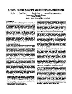
(a) CT (t) (b) ECT (t) Figure 6: Compact and extended compact trees ing in T , there is a tree Voronoi partition I with size less than 8Nw , where Nw is the number of nodes in T associated with w. Let us start the proof by introducing the compact tree of w, denoted as CT (w). First, all the nodes of U (w) are in CT (w), and termed the data nodes. Second, a non-data node u belongs to T , if and only if there are at least two child nodes of u whose subtrees contain a data node. We call u a branching node. Consider w = t in Figure 4. There are four data nodes 2, 5, 9, 23, and two branching nodes 1, 3. Node 17, for example, is not a branching node because only one of its child nodes (i.e., node 18) has a data node in its subtree. Let S be the set of all data and branching nodes. We form CT (w) by drawing an edge from each node u ∈ S to its lowest ancestor in S. Figure 6a shows the CT (t) for the data of Figure 4. Node 5, for instance, is connected to node 3, because among all the data and branching nodes, node 3 is the lowest ancestor of node 5. L EMMA 3. CT (w) has at most 2Nw − 1 nodes. P ROOF. Each branching node must have at least two child nodes in CT (w). As CT (w) has at most Nw leaf nodes, the total number of branching nodes cannot be more than Nw − 1. Consider any edge (u, v) in CT (w). Let us walk, in the data tree T , along the path from u to v. As we go, monitor the N N (z) of the node z being visited, and count how many changes in N N (z) there are in total. Call each of those changes an NN-change on (u, v). As an example, consider edge (1, 23) in the CT (t) of Figure 6a. Now we walk from node 1 to node 23 in the T of Figure 4. Along the path there is only a single NN-change, which happens as we move from node 17 to node 18 (i.e., N N (17) = 2, but N N (18) = 23). The next lemma gives an important fact: L EMMA 4. There can be at most one NN-change on each edge of CT (w). P ROOF. Let (u, v) be an edge of CT (w). The removal of (u, v) cuts CT (w) into two connected components. Let Cu (Cv ) be the component including u (v). Denote by P the path from u to v in T . Suppose that u⋆ (v ⋆ ) is the data node in Cu (Cv ) closest to u (v). We claim that, for any node z on P , N N (z) must be either u⋆ or v ⋆ . In fact, for any node u′ ∈ Cu , it holds that kz, u⋆ k = kz, uk + ku, u⋆ k ≤ kz, uk + ku, u′ k = kz, u′ k. Similarly, for any node v ′ ∈ Cv , we have kz, v ⋆ k ≤ kz, v ′ k. Therefore, except u⋆ and v ⋆ , no other data node in Cu ∪ Cv can be the NN of z. Hence, if there were at least two NN-changes on (u, v), there would have to be three nodes z1 , z2 , z3 on P such that z2 was on the path from z1 to z3 , but N N (z1 ) = N N (z3 ) 6= N N (z2 ). It is trivial to show that such a scenario cannot happen. Next, CT (w) is augmented with the nodes where NN-changes occur. Consider any edge (u, v) of CT (w) on which there is an

NN-change. Let z be the first node on the u-to-v path in T such that N N (z) 6= N N (u). If z is different from v, we add it to CT (w), breaking (u, v) into two edges (u, z) and (z, v). Denote by ECT (w) the resulting tree, after applying such transformation on all edges of CT (w) with NN-changes. In case root(T ) is not already in ECT (w), we add it as the parent of the current root of ECT (w). The final ECT (w) is called the extended compact tree of w. Let us illustrate the transformation with edge (1, 23) in the CT (t) of Figure 6a (i.e., u = 1, v = 23). As mentioned earlier, on the path from node 1 to node 23 in Figure 4, there is an NNchange as we cross from node 17 to node 18. Hence, z = 18, and accordingly, (1, 23) is broken into two edges (1, 18) and (18, 23) in the extended compact tree ECT (t), as shown in Figure 6b. We are ready to generate a tree Voronoi partition I of w. It suffices to invoke the following algorithm for every node u of ECT (w) in turn (ordering does not matter): algorithm voronoiIntv(u) /* u is a node in ECT (w) */ 1. S = {R(u)} 2. for each child node v of u in ECT (w) do 3. I ← the (only) interval in S covering R(v) 4. break I into intervals I1 , R(v), I2 /* I1 (I2 ) is the part of I to the left (right) of R(v) */ 5. remove I from S, and add I1 , I2 6. add to I the intervals in S, after associating them with N N (u)

For example, let u be node 1 in the ECT (t) of Figure 6b. At Line 1, voronoiIntv sets S = {R(1)} = {[1, 31]}. Since node 1 has two child nodes in ECT (t), the for-loop in Lines 25 is executed twice. The first time trims R(2) = [2, 16] away from [1, 31], after which S = {[1, 1], [17, 31]}. The second execution cuts R(18) = [18, 24] out of [17, 31], leaving S = {[1, 1], [17, 17], [25, 31]}. Line 6 adds all three intervals of S to I, after associating them with N N (1) = 2, indicating that node 2 is the NN of any node (whose rank falls) in those intervals. L EMMA 5. Applying voronoiIntv to all nodes of ECT (w) creates a tree Voronoi partition I with less than 8Nw intervals. P ROOF. We start by proving that the intervals of I are disjoint, and their union covers the rank domain D. Observe that the intervals inserted in I at Line 6 are disjoint with the R(v) of any child node v of u, where u is the input to the current execution of voronoiIntv. None of those intervals can overlap with the intervals added to I by the execution of voronoiIntv invoked with v (which only adds intervals within R(v)). On the other hand, every value x ∈ D is covered by an interval in the final I. Such an interval is inserted in I by running voronoiIntv with the lowest node u in ECT (w) whose R(u) covers x. We proceed to show that, for each interval I ∈ I, the NN associated with I is indeed the NN of all nodes in I. Consider any node u in ECT (w). Denote its child nodes in ECT (w) as v1 , ..., vf for some f ≥ 0. For each 1 ≤ j ≤ f , cutting R(vj ) out of R(u) at Line 4 effectively removes sub(vj ) from sub(u) (recall that sub(.) represents the subtree of a node). Let sub△ (u) be the set of nodes in sub(u), but not in the sub(vj ) of any j. It suffices to prove that all nodes in sub△ (u) have the same NN as u. For each edge (u, vj ) of ECT (w), define P (u, vj ) as the path in T from node u to vj , but excluding node vj . Each node z ∈ sub△ (u) is either (i) on P (u, vj ) for some j, or (ii) has an ancestor z ′ in T that is on P (u, vj ) for some j. In the former case, N N (z) must be N N (u) by the way ECT (w) is constructed. In the latter case, N N (z) = N N (z ′ ), while z ′ is a node of case (i), implying N N (z) = N N (u) as well.

It remains to bound the size of I. By Lemma 3, CT (w) has at most 2Nw − 2 edges. As each of them may generate two edges in ECT (w), the number of edges in ECT (w) is at most 4Nw − 4 + 1 = 4Nw − 3, including the (potential) extra edge due to root(T ). In voronoiIntv, each edge breaks D into at most 2 more intervals. Therefore, the final |I| is bounded above by 1 + 2(4Nw − 3) = 8Nw − 5. The proof of Theorem 1 is thus completed.

3.3 Finding the minimum TVP This subsection completes our discussion of NK search by elaborating an algorithm for computing a TVP I of a keyword w with the minimum size. In fact, the main idea of the algorithm has been mentioned in Section 3.2, as summarized below: algorithm computeTVP(w) 1. build CT (w) 2. build ECT (w) from CT (w) 3. I = ∅ 4. for each node u in ECT (w) do 5. voronoiIntv(u) /* at the end of the for-loop, |I| < 8Nw */ 6. merge consecutive intervals in I that are associated with the same NN 7. return I

Next, we clarify the details of Lines 1 and 2, because voronoiIntv has been presented in the previous subsection. Construction of CT (w). We construct CT (w) in two steps: first collect the set S of nodes in CT (w), and then connect them properly to meet the definition of CT (w). The first step applies the algorithm below to compute S: algorithm collectCTnodes(U (w)) 1. S = U (w) 2. sort the nodes of U (w) in ascending order of ranks 3. for each pair of consecutive nodes u, v do 4. S = S ∪ lca(u, v)

We claim that the final S includes all the branching nodes. Let z be any branching node. By definition, it has at least two child nodes that have a data node in their subtrees, respectively. Let u1 , u2 be the two left-most ones of those child nodes, with u1 being the left-most one. Denote by v1 (v2 ) the data node with the largest (smallest) rank in the subtree of u1 (u2 ). By the property of preorder ranking, v1 and v2 constitute a pair of consecutive data nodes in the rank domain. Hence, z will be discovered as lca(v1 , v2 ). Recall that each node in CT (w) should be connected to its lowest ancestor (if any) among all the nodes in CT (w). We achieve the purpose using a stack J. Specifically, we process the nodes of S in ascending order of their ranks, and maintain CT (w) for the nodes already seen. At each moment, J keeps the right-most root-to-leaf path of the current CT (w). Nodes of the path are pushed in J in the same order they are scanned, i.e., with the leaf (root) at the top (bottom). algorithm computeCTedges(w) 1. sort the nodes of S in ascending order of ranks 2. J = ∅ 3. while S 6= ∅ do 4. u ← the first node of S; remove u from S

5. 6. 7. 8.

keep popping the top node v of J as long as R(v) is disjoint with R(u) if J is not empty then add an edge between u and the top node of J push u in J

Let us illustrate the algorithm using the set of nodes in the CT (t) of Figure 6a. Here, S = {1, 2, 3, 5, 9, 23}. Node 1 is the first scanned, and directly pushed to J. For node 2, Line 5 has no effect, while Lines 6-7 add an edge between nodes 1 and 2. J = {2, 1} at this time (with node 2 at the top). Similarly, the scanning of nodes 3 and 5 create edges (2, 3) and (3, 5) respectively, after which J = {5, 3, 2, 1}. Next, the algorithm comes to node 9. Line 5 pops node 5 out of J because R(5) is found to be disjoint with R(7). Line 6 then spawns another edge (3, 9) in CT (t). Finally, the handling of node 23 pops nodes 9, 3, 2, and adds one more edge (1, 23). The CT (t) now becomes final as S has been exhausted. Construction of ECT (w). Let (u, v) be an edge in CT (w), with u being an ancestor of v. Lemma 4 states that there can be at most one NN-change on (u, v). In case no NN-change exists, (u, v) is kept directly in ECT (w). Otherwise, we should create two edges (u, z), (z, v) in ECT (w), where z is the first node (on the u-to-v path in T ) such that N N (u) 6= N N (z). Our algorithm for building ECT (w), named computeECT, processes the edges (u, v) of CT (w) in ascending order of level(u). It keeps the invariant that, at the time (u, v) is to be processed, we have already determined N N (u). It is easy to see that N N (v) can only be either N N (u) or N Nsub (v), where N Nsub (v) is the subtree nearest w-neighbor of u (see Section 2). Another key to the algorithm is that, if N N (v) turns out to be different from N N (v), the node z splitting (u, v) can be identified by a level-on-path query. This is because the level ℓ of z can be calculated as:   δ + level(u) + level(v) ℓ= (1) 2 where δ = kv, N N (v)k − ku, N N (u)k. algorithm computeECT(CT (w)) 1. sort the edges (u, v) of CT (w) in ascending order of level(e); E ← the sorted list 2. find the NN of the root of CT (w) with a subtree NK query 3. while E 6= ∅ do 4. (u, v) ← the first edge of E; remove it from E 5. N Nsub (v) ← the subtree nearest w-neighbor of v 6. N N (v) ← whichever of N N (u) and N Nsub (v) that is closer to v 7. if N N (u) = N N (v) then 8. create edge (u, v) in ECT (w) 9. else 10. z ← the result of a level-on-path query using (u, v) and ℓ (Equation 1) 11. create edges (u, z) and (z, v) in ECT (w)

We demonstrate the algorithm by explaining how to derive the ECT (t) in Figure 6b from the CT (t) in Figure 6a. First, Line 1 arranges the edges of CT (t) in the order of E = {(1, 2), (1, 23), (2, 3), (3, 5), (3, 9)}. Line 2 obtains N N (1) = 2. The subsequent execution examines each edge of E in turn. The first one, (1, 2), is easy to handle because N N (2) = N N (1) = 2. Hence, (1, 2) is included in ECT (t) directly. Consider the second edge (1, 23) of E. As N N (23) = 23 is different from N N (1), Line 10 calculates ℓ = ⌈(−1 + 0 + 4)/2⌉ = 2, and issues a levelon-path query to find the level-2 node z on the path from node 1

to node 23 in the data tree of Figure 4. The z retrieved is node 18. Line 11 then adds edges (1, 18) and (18, 23) into ECT (t). The rest of the algorithm proceeds in the same manner. Analysis. Line 1 of computeTVP invokes collectCTnodes and computeCTedges, both of which terminate in O(Nw log Nw ) time. The same complexity applies to at Line 2, which executes computeECT. Lines 4-5 essentially spend constant time on each edge of ECT (w), and hence, incur only O(Nw ) cost. Line 6 apparently requires O(Nw ) time. Therefore, the overall complexity of computeTVP is O(Nw log Nw ). T HEOREM 2. T can be pre-processed into a structure that occupies O(K) space, such that any NK query can be answered in O(log Nw ) time, where Nw is the number of nodes in T carrying the query keyword. The structure can be built in O(K log K) time. P ROOF. The result follows from the discussion in Section 3.1, Theorem 1, the analysis of this subsection, and the fact that (i) theP total construction cost of the structures of all keywords is O( w (Nw log Nw ))P= O(K log K), P and (ii) the space of all these structures is O( w Nw ) = O( u |W (u)|) = O(K). When B-trees, instead of binary trees, are deployed, the space and query complexities of our structure are O(K/B) disk blocks and O(log B Nw ) I/Os, respectively, where B is the size of a block.

4. NEAREST KEYWORD SEARCH AS AN OPERATOR In the introduction, we outlined why NK search can be deployed as a primitive operator to support other tasks efficiently. Sections 4.1 and 4.2 elaborate this for XPath query answering and group steiner tree computation, respectively.

4.1 XPath evaluation This subsection aims at a theoretical justification that many XPath queries can be reduced to NK search. We consider queries that can be represented as a twig pattern Q as follows. Each internal node of Q gives an element type. A leaf node is designated as the output, indicating the information solicited (extension to multiple output nodes is trivial). Every other, non-output, leaf node carries a keyword, which imposes a predicate that must hold on each occurrence of Q in the data tree T . See Figure 2a for an example. Without loss of generality, we assume that Q is compatible with the data schema; otherwise, it can be rejected by standard syntax checking with the DTD. We will prescribe two conditions whose satisfaction guarantees the success of reducing Q to a set of NK queries. These conditions are conservative, in the sense that one may still carry out reduction even if the conditions do not hold (as shown in the experiments). We will see that the class of reducible queries can be processed by a new algorithm with an attractive worst-case performance bound. Type-sequence condition. Let P be any path of T starting from root(T ). Define the type sequence of P as the ordering of the node types encountered as we walk along P . For instance, if P is the path from node 0 to node 010 in Figure 1, its type sequence is (league, team, tname). C ONDITION 1. For each node u of the same type, the root-to-u path in T has the same type sequence. In Figure 1, for example, the path from the root to every player node has type sequence (league, team, players, player).

team division

player

divisionVal pname

from

pnameVal fromVal

Figure 7: Type pattern of the query in Figure 2a Anchor condition. As the next condition is more complex, we first explain the idea using an example. Consider Q to be the pattern in Figure 2a. Let us examine its type pattern, which is also a tree, and results from replacing each node of Q with its type, as shown in Figure 7. Denote the type pattern of Q as type(Q). Let us fix a leaf node, fromVal, in type(Q) as the anchor, denoted as anc. Then, find the LCA, called a critical LCA, of anc and every other leaf, namely, (i) clca1 = team, which is the LCA of anc and leaf1 = divisionVal, and (ii) clca2 = player, which is the LCA of anc and leaf2 = pnameVal. Each pair (clcai , leafi ) decides a critical set represented as cseti , which includes all the types on the path from clcai to leafi . That is, cset1 = {team, division, divisionVal}, and cset2 = {player, pname, pnameVal}. In the T of Figure 1, for each type-clcai node u, sub(u) (i.e., the subtree of u) has at most one node of each type in cseti . To be specific, let us inspect clca1 = team. The subtree of a team node can have at most one node of type team, division, and divisionVal, respectively. Similarly, this is also true for clca2 , i.e., every player node can have in its subtree at most one player, pname, and pnameVal node, respectively. In this case, we say that Q is unambiguous. Not all the choices of anc would make Q unambiguous. For example, it is not hard to see that Q is not unambiguous if divisionVal is selected as the anchor. The second condition requires: C ONDITION 2. At least one choice of anchor makes Q unambiguous. To grasp the intuition behind the condition, consider again the strategy explained in Section 1.1 for processing the query Q of Figure 2a. Recall that we used the fromVal nodes carrying Maryland as the query nodes q for NK search. Instead, let us choose q as the divisionVal nodes associated with west. That is, for each such q, say node 0100, the algorithm finds its nearest Maryland-neighbor (i.e., node 012020) in the set of fromVal nodes, and then checks whether the neighbor has distance 6 to q. The answer is yes, so the presence of an occurrence has been detected. The problem, however, is that we can no longer find the output value Blake by identifying the nearest pnameVal-neighbor of q. This is because multiple pnameVal nodes have an identical (smallest) distance 6 to q and, hence, the NK search with pnameVal as the query word may happen to return a node (e.g., 012100) that is not describing the same player as node 012020. We point out that, although the definitions and notations leading to Condition 2 were introduced with an example, they can be generalized in a straightforward manner to arbitrary Q. Reducibility. The theorem below formally establishes the reduction from XPath evaluation to NK search. T HEOREM 3. An XPath query can be reduced to NK search under Conditions 1 and 2. P ROOF. As in Section 1.1, we set the type of each node u in T as a keyword in u. Each value node has its value as an extra keyword. An XPath query Q is processed with the following algorithm:

algorithm xpath(Q) 1. for each node q in T having type anc do 2. for each non-output leaf node u of Q do 3. w ← the keyword of u 4. v ← the result of N N (q, w) among all nodes in T of the same type as u /* This can be done with minor extension to our technique in Section 3. For example, one simple solution is to prefix each word with the type of the node containing it. Such a prefix is added to w, which automatically restricts the search to the nodes of the designated type. */ 5. if kq, vk 6= the correct value as in an occurrence then 6. mark q as pruned 7. break for 8. if q has not been pruned then 9. w ← the type of the output node of Q 10. v ← N N (q, w) 11. if kq, vk = the correct value as in an occurrence then 12. report the value of v

Let us refer to the type-anc node in an occurrence of Q as an anchor node. Denote by f be the number of leaf nodes in type(Q) other than anc. Lines 2-12 of xpath are collectively called an iteration. We will prove that (a) the output value in every occurrence is reported by xpath, and (b) every value reported is indeed the output value of an occurrence. Proof of statement (a). Let occ be any occurrence with q as its anchor node. Denote by ui the type-leafi node in occ (1 ≤ i ≤ f ). Each ui must be retrieved by the NK-query at Line 4 (or 10) in the iteration for q, and pass the if-condition at Line 5 (or 11). The iteration reports the output value of occ at Line 12. Proof of statement (b). Under Condition 1, it suffices to consider Q with single-lined edges only, because any double-lined edge can be expanded into a set of single-lined edges without affecting the query result. Condition 1 also allows us to focus on Q (i) that has only a single node, or (ii) whose root has at least two child nodes. If root(Q) has a single child, we can remove the root while still obtaining the same result. Assume that xpath reports a value in an iteration with q as the anchor node. Line 4 or 10 must have fetched a type-leafi node ui (1 ≤ i ≤ f ). Let occ be the tree that (i) is rooted at the LCA of u1 , ..., uf , q, and (ii) includes (only) the edges on the path from the LCA to each of u1 , ..., uf , q. The rest of the proof argues that occ is an occurrence. Towards this, we consider tree type(occ), which is obtained by replacing each node of occ with its type. Our goal is to show that type(occ) and type(Q) are exactly the same. Condition 1 implies that all nodes of a type must be at the same level. Given a node type z, we use seq(z) to represent the type sequence of the path in the data tree T that goes from the root (of T ) to an arbitrary type-z node u (recall that seq(z) is unique regardless of u). Also, suppose that clca1 , ..., clcaf are in the topdown order. As clcai ∈ seq(anc) for each i ∈ [1, f ], q has a (unique) typeclcai ancestor in T , which we represent as vi . A key observation is that ui must be in the subtree of vi . Otherwise, kq, ui k would have been at least 2 more than the correct value in an occurrence, noticing that the path from q to ui would need to go outside sub(vi ), and then eventually descend to the level where type-leafi nodes are. From type(Q), we know that clcai is the last common type in seq(leafi ) and seq(anc), implying that vi must be the LCA of ui and q, and belong to occ. Hence, the root of occ has type clca1 . Let PQ (or Pocc ) be the path in type(Q) (or type(occ)) from the root to anc. The earlier analysis indicates that PQ is identi-

cal to Pocc . Next we prove that type(occ) and type(Q) are the same in the other parts as well. Let us walk down PQ and Pocc synchronously, and stop as soon as encountering a clcai (of any i ∈ [1, f ]) in both paths. Let TQ (or Tocc ) be the subtree of clcai in type(Q) (or type(occ)), removing the subtree rooted at z, where z is the child node of clcai that is an ancestor of anc. Define S = {j | clcaj = clcai } (it is possible for several critical LCAs to coincide on one node). Let z be any type in the csetj of any j ∈ S. Under Condition 2, there is a unique type-z node in the subtree of vi in T . Therefore, each type in TQ (Tocc ) can appear only once. For each leafj (j ∈ S), define a type-sequence sj that equals the suffix of seq(leafj ) starting from clcai . Regarding each type as a symbol, both TQ and Tocc are in fact a trie of the same set of strings {sj | j ∈ S}. The above reasoning of TQ and Tocc is independent of i. We thus have established the equivalence of type(Q) and type(occ).

Remark 1. We outline the main ideas on how to verify Conditions 1 and 2 efficiently, while leaving the complete details to the full paper. We regard each rule of the DTD as having the form e → s, where e is an element type and s a string specifying the possible child element types of e. Combine multiple rules whose left hand sides are the same type. Denoting by S the set of resulting rules, we can show that Condition 1 is satisfied if and only if every element type appears on the right hand side (RHS) of exactly one rule in S. To check Condition 2, we resort to a schema tree ST , where each node is an element type e, whose child nodes are the element types in the RHS of rule e → s. Recall that every element type c in s may carry a star (e.g., e → c∗ means that there can be multiple instances of c below e directly). In this case, the edge (in ST ) from e to c is a star edge; otherwise, it is a non-star edge. Given a query Q, ST allows us to verify Condition 2 as follows. First pick a leaf node of type(Q) as the anchor anc. Perform the following for every other leaf node u: identify the LCA v of anc and u, and examine if the path from v to u in ST has a star edge. If the answer is no for all u, we assert that Q satisfies Condition 2. Otherwise, pick a different anchor and repeat the above process. If all anchors have been attempted and Q has not been confirmed to satisfy Condition 2, we conclude that it violates the condition. Clearly, the time of Condition-2 checking depends only on the schema, is irrelevant to the size of the XML document, and hence, typically accounts for only a fraction of the total query cost. Note that Condition 1 (2) is a constraint on the data (queries). It is worth mentioning that the two conditions are satisfied by many real datasets and meaningful queries. In particular, we note that all the datasets experimented in [4, 6, 10, 34, 35] and at least one in [7, 15, 16, 20, 27, 28, 29, 30, 32, 37] satisfy Condition 1 (see also our experiments). We point out that simple aliasing can often be carried out to make a dataset satisfy Condition 1. For example, in the well-known DBLP dataset, an author element may be under an article or inproceedings element. To meet Condition 1, we can rename the author of former type as a-author, and that of the latter type as i-author. Remark 2. Denote by leaf1 , ..., leaff the leaf nodes of Q that are not the anchor P anc. By Theorem 2, algorithm xpath terminates in O(Nanc fi=1 log Nleafi ) time, where Nx is the number of nodes in the data tree T fulfilling the predicate implied by the node x in type(Q). For example, for the Q of Figure 2a, the execution time is O(NMaryland (log Nwest + log NpnameVal )). In general, the time complexity of xpath is independent on the number of nodes in T whose types are internal nodes of type(Q). This is a unique performance characteristic that is not shared by any previous solution.

4.2 Finding approximate group steiner trees This section discusses the GST problem as motivated in Section 1. The dataset is a tree T as described in Section 2. A query specifies a set of keywords QS = {w1 , ..., wl }. Recall that U (wi ) is the set of nodes in T associated with wi (1 ≤ i ≤ l). Any l nodes u1 , ..., ul , where ui ∈ U (wi ) for each i, uniquely determines a minimum connecting tree (MCT) [20] M as follows. M has the LCA of all u1 , ..., ul as its root, and includes (all and only) the edges on the path in T from the LCA to every ui . Referring to (u1 , ..., ul ) as a vector, the GST problem is equivalent to discovering the vector that minimizes the number of edges in M . This problem is NP-hard [17]. As an example, assume T to be the data tree in Figure 1, and w1 = Lakers, w2 = Blake, w3 = guard (l = 3). Given u1 = node 0100, u2 = node 012000, and u3 = node 012010, Figure 3 demonstrates the corresponding MCT M . Notice that the root of M is the LCA of u1 , u2 and u3 . We assume that w1 , ..., wm have been arranged in such a way that |U (w1 )| ≤ ... ≤ |U (wl )|. The following algorithm extracts an MCT with a small number of edges. algorithm approxGST(w1 , ..., wl ) 1. dmin ← ∞ 2. for each node u1 ∈ U (w1 ) do 3. for i ← 2 to l do 4. ui ← N N (u1 , wi ) P 5. d ← li=2 ku1 , ui k 6. if d < dmin then 7. remember (u1 , ..., ul ) as the best vector 8. dmin = d 9. return the MCT M determined by the best vector

The for-loop in Lines 2-8 enumerates each node u1 ∈ U (w1 ). Lines 3-4 find the nearest wi -neighbor of u1 for every other query keyword wi . The resulting neighbors, together with u1 , determine an MCT. The key of the algorithm is to measure the quality of the tree as the sum of the distance from u1 to each retrieved neighbor (see Line 5). The algorithm eventually returns the best tree according to this quality metric. We say that an MCT M is a c-approximate GST if it has at most c times more edges than the GST. Formally, if cost(M ) represents the number of edges in M , it holds that cost(M ) ≤ c · cost(M ⋆ ), where M ⋆ is the (optimal) GST. L EMMA 6. The output of approxGST is an (l − 1)approximate GST. P ROOF. For each i ∈ [1, l], let u⋆i be a node in M ⋆ associated with keyword wi (if there such nodes, u⋆i can be any of Pl are several ⋆ ⋆ ⋆ them). Define d = i=2 ku1 , ui k. Since every edge of M ⋆ is included at most once in the path from u⋆1 to each u⋆i (2 ≤ i ≤ l), it holds that: d⋆ ≤ (l − 1) · cost(M ⋆ ).

(2)

Let Mapx be the output of approxGST. The dmin in the sequel refers to the final dmin of approxGST. Notice that {u⋆1 , N N (u⋆1 , w2 ), ..., N N (u⋆1 , wl )} is a set {u1 , ..., ul } that must have been inspected at Line 5 of approxGST. In other words: dmin ≤

l X

ku⋆1 , N N (u⋆1 , wi )k ≤ d⋆ .

(3)

i=2

where the second ≤ is because ku⋆1 , N N (u⋆1 , wi )k ≤ ku⋆1 , u⋆i k.

Let {ˆ u1 , ..., u ˆl } be the set {u1 , ..., ul } that determines Mapx at Pl Line 7 of approxGST. Then, dmin = u1 , u ˆi k. Every i=2 kˆ edge of Mapx is used at least once in the union of the paths from u ˆ1 to u ˆ2 , ..., u ˆl , respectively. Hence: cost(Mapx ) ≤ dmin .

(4)

Combining Inequalities 2-4 gives cost(Mapx ) ≤ (l − 1) · cost(M ⋆ ). By Theorem 2, the execution time of approxGST is bounded by O(Nmin l log Nmax ), plus the cost of outputting the tree, where Nmin = |U (w1 )| and Nmax = |U (wl )|. Remark 3. Sometimes it is useful to return k MCTs with small cost, where k is a user-specified parameter. In this case, we maintain the k best vectors currently found, as opposed to only the top-1. This can be achieved with minor modification to approxGST.

5.

RELATED WORK

NK search has not been studied previously. In the sequel, we review the existing work on other topics related to our discussion. The first topic is the processing of holistic twig joins, where the goal is to enumerate all occurrences of a twig pattern. The existing algorithms can be classified as sequential or indexed. A sequential algorithm [4, 5, 8, 7, 15, 21, 30, 32, 37] scans synchronously the nodes, whose types appear in the query pattern, in ascending order of their ranks. The drawback of these algorithms is that they must access every such node at least once, even though it does not participate in any occurrence. Motivated by this, an indexed algorithm [4, 21] utilizes a data structure that can be used to efficiently retrieve a particular ancestor/descendent of a node. Such an ability allows the algorithm to skip many nodes not involved in any occurrence and, therefore, to terminate much earlier. In this paper, we do not attempt to attack general holistic twig joins. Instead, our focus is to improve the efficiency of those XPath queries that can be processed with NK search. As far as these queries are concerned, our method significantly outperforms all the solutions in the sequential category because (similar to indexed algorithms) it only needs to access a small number of nodes that may form an occurrence. Regarding the indexed category, the comparison is more subtle, mainly because the algorithms of [4, 21] are heuristic in nature, and are not accompanied by any nontrivial complexity analysis. We will experimentally compare our technique against the state of the art, TSGeneric+ [21], of that category. Noteworthily, an advantage of our algorithm xpath (Section 4.1) is that, in practice, its cost can be accurately estimated by a query optimizer. This is not possible for [4, 21], as their behavior is sensitive to the data distributions. We note that no existing algorithm has the performance characteristic pinpointed in Remark 2. The only approach that comes close to having the characteristic is TJFast [30], which is a sequential algorithm that needs to scan the nodes matching only the leaves of the query pattern. Unfortunately, the extended dewey codes that TJFast relies on can be as long as the height of the XML tree. The time of reading a node is proportional to the length of its extended dewey code. The length, unfortunately, is linear to the number of ancestors of the node, which can be asymptotically identical to the total number of nodes in the tree in the worst case. It is also worth mentioning that there exist some other methods [9, 24], just like ours, that are designed for certain special classes of XPath queries. Another related topic is keyword search in XML databases. A bulk of the existing research [6, 10, 16, 20, 27, 28, 29, 35] explores various semantics of query results that is suitable for different scenarios. In this work, we showed the applicability of NK search to

the GST semantics [12, 20, 23, 25]. This choice does not imply our preference of GST; in fact, the potential application of the NK operator to the other semantics is an exciting direction for future work. As mentioned before, the GST problem on trees is NP-hard, and remains so even if the goal is changed to finding an O(log2−ǫ n)approximate solution for arbitrarily small ǫ > 0 [17], where n is the number of nodes in the data tree. The best known approximation ratio achievable in polynomial time is O(log n log l) [14], where l is the number of query keywords (and can be as large as n). The algorithm of [14], which is based on linear programming, is highly theoretical and not appropriate for practical implementation. In the database area, research on GST computation (e.g., [3, 12, 19, 20, 22, 25]) is largely motivated by the observation that the value of l can often be regarded as a constant in reality. In this case, the l−1 approximation ratio guaranteed by our solution (Lemma 6) can be (much) lower than O(log n log l). A small l also considerably shrinks the search space for discovering the GST. This fact is leveraged in [20] to enumerate all the MCTs (defined in Section 4.2), and thereby, eventually come across the GST (which is also an MCT). While the method of [20] works on trees only, the approaches reviewed below apply to general graphs1 . Algorithms for computing approximate GSTs (faster than extracting the GST with [20]) are presented in [3, 22]. Somewhat surprisingly, there is a dynamic-programming algorithm [12] for finding the exact GST, in even less time than the approximate methods of [3, 22]. The above approaches do not rely on pre-computation, whereas the BLINKS system [19] leverages a sophisticated access method constructed in advance to produce l-approximate GSTs efficiently. The most serious drawback of BLINKS, however, is that it occupies Ω(n4/3 ) space2 , where n is the number of nodes in the graph. For n at the order of millions, Ω(n4/3 ) amounts to duplicating the database 100 times, which is too expensive in many environments. Furthermore, the query algorithm of BLINKS is ad-hoc and has no interesting worst-case performance bound. Note that our result in Lemma 6 in fact dominates the performance of BLINKS, i.e., we guarantee a slightly better approximation ratio, with a linear space access method and worst-case efficient query time. It should be noted, however, that the improvement is made possible by utilizing properties of a tree (recall that BLINKS deals with general graphs). The work of [23, 25] considers the steiner tree problem, which is a special case of the GST problem where there can be only a single node in the data tree associated with each query keyword. Note that, while the steiner tree problem is NP-hard on graphs, it is not on trees, as is clear from the way that MCT is built from a vector in Section 4.2. Finally, in the special case where only one distinct keyword exists, NK retrieval is similar to nearest neighbor search on spatial networks. In that problem, the data consist of a graph G and a set S of points, each located at a node of G. Given a node q of G, a query returns the point in S that has the smallest shortest-path distance to q. This problem has been well studied in various settings with different performance goals (see [11, 26, 31, 33] and the references therein). The existing solutions (i) perform Dijkstra-like expansion from the query point (e.g., [11]), (ii) pre-compute the answer for each node of G (e.g., [31]), or (iii) rely on specialized structures that leverage properties of spatial data (e.g., [26, 33]). In our con1

Given a set of keywords, the GST in a graph is the minimum tree (i) whose nodes and edges come from the underlying graph, and (ii) that has the minimum number of edges among all trees satisfying (i). When the graph is a tree, this definition degenerates into the one in Section 4.2. 2 This can be derived from Theorem 3 of [19] by observing that, P 2 2 2 4/3 ). b Nb + BP ≥ n /B + B , which is Ω(n

text, solutions of (i) degenerate into the BFT approach explained in Section 3.1, those of (ii) incur prohibitive space when the number of keywords is large, whereas those of (iii) are simply inapplicable to XML data.

6.

EXPERIMENTS

This section empirically evaluates the performance of the proposed techniques. We used two real XML documents: • NBA, which contains all the teams and players of the leagues during 1946-2004. • DBLP, which includes all the conference papers during 1959-2010 collected by the DBLP website. Figure 8a (8b) shows the part of the NBA (DBLP) schema that is relevant to the queries in our experiments. An asterisk indicates that the corresponding node can have an arbitrary number of siblings of the same type. For example, an NBA node can have multiple child nodes of type league. Table 1 lists the main statistics about each dataset.

league*

DBLP

team*

inproceedings*

year division tname players year author* title booktitle yearVal divisionVal tnameVal player* yearVal booktitleVal titleVal authorVal position

DBLP 759 427

NBA < 1 second

DBLP < 2.5 minutes

Table 3: Construction cost of Table 2: Space (mega bytes) TVP N Q1: Find the team of Shaquille O’Neal in 2000. q = the pnameVal node with value Shaquille-O’Neal in the league 2000; w = tnameVal N Q2: Were Shaquiile O’Neal and Kobe Briant in the same team in year 2000? q = same as N Q1; w = pnameVal:Kobe-Bryant; distance (of a positive answer) = 6 N Q3: Same as N Q2 but in 2002. q = same as N Q1 but in 2002; w and distance as in N Q2 DQ1: Find the conference name of “Holistic Twig Joins: Optimal XML Pattern Matching”. q = the ptitleVal node of the paper; w = booktitleVal DQ2: Is Nicolas Bruno an author of the paper in DQ1? q = same as DQ1; w = authorVal:Nicolas-Bruno; distance = 4 DQ3: Same as DQ2 but with respect to Jim Gray. q and distance same as DQ2; w = authorVal:Jim-Gray

query, Figure 9 clarifies the node q and keyword w of the corresponding NK operator. For a boolean query, the figure also points out the distance (to q) that the nearest w-neighbor should have in order to return a positive answer. For instance, the answer for N Q2 is “yes” if and only if the retrieved neighbor has distance 6 to q. 1000000

college

pnameVal positionVal collegeVal

(a)

NBA 3.8 2.4

Figure 9: Query set for examining NK efficiency

NBA

pname

TVP raw dataset

(b)

Figure 8: Schemas of NBA and DBLP relevant to our queries NBA DBLP num. of nodes 135,940 17,501,788 num. of keywords 223,500 48,191,004 num. of distinct keywords 8,302 2,893,195 Table 1: Dataset statistics We will first explore the characteristics of NK search, and then assess the usefulness of the NK operator in XPath evaluation and GST computation, respectively. Our experiments were performed on a computer that was running Linux, and equipped with an Intel DUO CPU at 3.0Ghz and 4 GB of memory. All the data were memory resident. Performance of NK search. In our indexing scheme, named TVP, we followed the convention mentioned in Section 1.1 to associate nodes with keywords. Specifically, every node had its type as a keyword. Furthermore, if u is a value node, each word w in the value of u was taken as another keyword of u, after w was prefixed with the type of u (see Remark 1 of Section 4.1). The name of a person/team was always regarded as a single word. For instance, if u has type pnameVal and a value Kobe Bryant, then it carries a (prefixed) keyword pnameVal:Kobe-Bryant. Table 2 shows the space consumption of TVP and the raw dataset, while Table 3 gives the construction time of TVP. The next experiment compares the query efficiency of TVP and the BFT algorithm described in Section 3.1. For this purpose, we report their performance on the (realistic) queries in Figure 9, each of which can be handled by a single NK operator. Queries denoted with a first letter N (D) were designed for NBA (DBLP). For each

cost ( µ sec)

TVP

BFT

100000 10000 1000 100 10 1 0.1 0.01 NQ1

NQ2

NQ3

DQ1 DQ2

DQ3

Figure 10: Cost of NK search Figure 10 illustrates the cost of TVP and BFT for each query. Note that the vertical axis is in logarithmic scale, and has the unit of µ-second (= 10−6 second). BFT is especially slow for the boolean queries N Q3 and DQ3 with answers “no”. This is expected because, for these queries, the retrieved neighbor has a large distance to the query node. XPath evaluation. We proceed to assess the efficiency of the NK operator in answering XPath queries. Our technique integrated the proposed access method TVP with the xpath algorithm developed in Section 4.1. As discussed in Section 5, the existing algorithms for holistic twig joins can be classified into the sequential and indexed categories, with the solutions in the latter category significantly faster than those of the former. Therefore, we chose to compare TVP against the state-of-the-art indexed algorithm TSGeneric+ [21]. Figures 11a and 11b explain the meaning and twig patterns of the queries examined, respectively. The box in each pattern signifies the anchor node chosen by xpath. Observe that N Q7 and DQ7 violate the anchor condition (i.e., Condition 2) in Section 4.2. Nevertheless, they are still reducible to NK search and, in fact, can be answered directly by the xpath algorithm with no modification. For fairness, our implementation of TSGeneric+ utilizes an inverted index to filter all the nodes that do not satisfy the keyword conditions. For example, for N Q4, only the collegeVal nodes

N Q4: Find the names of all players from Duke University. N Q5: Find the names of all centers from the west division. N Q6: Find the names of all players that came from Boston College but were in a team of the west division in year 1999. N Q7: Find the teams where Hakeem Olajuwon and Charles Barkley were teammates. DQ4: Find the titles of all papers by Jim Gray. DQ5: Find the titles of the SIGMOD papers by Nick Koudas. DQ6: Find the conferences of the papers by Divesh Srivastava that contained “XML” in the titles. DQ7: Find the titles of the SIGMOD papers co-authored by Hector Garcia-Molina and Jennifer Widom.

(a) Query description N Q4

N Q6

team N Q5 player division pname pos west pnameVal center

player pname college pnameVal Duke league year

team

player division 1999 pname college west

tname tnameVal

team player Hakeem Olajuwon

N Q7 player Charles Barkley

pnameVal Boston DQ4

inproceedings author title titleVal Jim Gray

title

inproceedings DQ5 booktitle author

titleVal

SIGMOD Nick Koudas

inproceedings inproceedings DQ7 DQ6 title booktitle author author booktitle title author Divesh titleVal SIGMOD Hector Jennifer booktitleVal XML Srivastava Garcia- Widom Molina

(b) Twig patterns Figure 11: Query set for examining XPath efficiency 672 1431 cost ( µ sec)

200 180 160 140 120 100 80 60 40 20 0

~~

TVP

TSGeneric+

NQ4 NQ5 NQ6 NQ7 DQ4 DQ5 DQ6 DQ7

Figure 12: Cost of XPath queries whose values are equal to Duke are considered, as opposed to all the collegeVal nodes (as proposed in [21]). This optimization reduces the average overhead of the original TSGeneric+ by at least an order of magnitude. Figure 12 demonstrates the execution time of TVP and TSGeneric+ for all queries. TVP lost narrowly in two out of the eight queries, but was at least twice faster in four queries. GST computation. The final set of experiments investigate the efficiency and effectiveness of the NK operator in keyword search. Our approach combined the TVP indexing scheme with the approxGST algorithm in Section 4.2. We compared the approach against the dynamic programming algorithm of [12] (as reviewed in Section 5), hereafter denoted by DP. Recall that DP returns the exact GST. We evaluated the two methods only with NBA, as the excessive memory requirements of DP rendered it infeasible to run experiments with DBLP on our hardware. As the XML schema is irrelevant to keyword search, the TVP built here does not require the keyword prefixing explained earlier. In other words, each element node (as before) is associated with its type, whereas each

N Q8: {Shaquille-O’Neal, Anfernee-Hardaway} N Q9: {Shaquille-O’Neal, Anfernee-Hardaway, Orlando-Magic} N Q10: {Shaquille-O’Neal, Anfernee-Hardaway, Orlando-Magic, 2000}

Figure 13: Query set for keyword search evaluation # of edges

16 14 12 10 8 6 4 2 0

TVP

DP

1.07 approx. ratio

1

cost (msec)

TVP

100000 10000 1000 100

DP

10 1 0.1

1

NQ8

NQ9

0.01 0.001

NQ8

NQ10

NQ9

NQ10

(a) Number of edges (b) CPU time Figure 14: Quality and efficiency of GST computation value node is simply associated with the words in its value. Figure 13 illustrates the queries executed. Figure 14a depicts, for each query, the number of edges in the trees output by TVP and DP, respectively. It also indicates the approximation ratio of TVP. Notice that TVP returns the exact GST for N Q8 and N Q9, whereas its result for N Q10 has one more edge than the optimal solution. This shows that, in practice, the actual approximation ratio of TVP is much better than predicted by theory (Lemma 6). Figure 14b plots the CPU time of the two methods. TVP outperforms DP by two to five orders of magnitude. Moreover, unlike DP whose cost surges with the number of query words, the overhead of TVP is only slightly affected. To better capture the usefulness of TVP in keyword search, Figure 15 presents the trees returned by TVP in the previous experiment. The result of N Q8 essentially states that Shaquille-O’Neal and Anfernee-Hardaway played for the same team at least once in their career. The tree of N Q9 implies that the above players were once teammates in Orlando-Magic. Finally, the N Q10 result indicates that Shaquille-O’Neal and Anfernee-Hardaway belonged to different teams in 2000, neither of which was Orlando-Magic. We conclude our experiments by comparing TVP and DP in searching for the top-k GSTs of N Q9 with k > 1. TVP now modifies approxGST as discussed in Remark 3. Note that both TVP and DP are approximate, namely, DP guarantees returning the top1 GST, but such optimality is not ensured for k > 1. Figure 16a plots the result quality (in the number of tree edges) as a function of k. The two algorithms output trees with identical sizes when N Q8

players

team

player

player

pname

pname

Shaquille-O′ Neal

Anfernee-Hardaway

N Q9 tname Orlando-Magic

players player

player

pname

pname

Shaquille-O′ Neal

Anfernee-Hardaway

league

N Q10 team players

team players

team

year

tname

2000

player

player

Orlando-Magic

pname

pname

Shaquille-O′ Neal

Anfernee-Hardaway

Figure 15: MCTs returned by TVP for the queries of Figure 13

# of edges

TVP

16 14 12 10

DP

TVP

DP

100 10 1 0.1 0.01 0.001

8 6 4 2 0

cost (msec)

100000 10000 1000

1

2

3 k

4

5

(a) Number of edges

1

2

3 k

4

5

(b) CPU time

Figure 16: Quality and efficiency of top-k GST computation k ∈ [1, 3], whereas DP offers slightly smaller trees for k ∈ [4, 5]. Figure 16b gives their CPU cost. The overhead for both methods gradually elevates with k. TVP constantly outperforms DP by more than four orders of magnitude.

7.

CONCLUSIONS

This paper proposed the problem of NK search on XML documents. Given a node q and a keyword w, an NK query returns the node in the XML tree that has the shortest distance to q, among all nodes associated with w. We solved the problem with a novel technique called tree Voronoi partition that gives rise to an indexing scheme with rigorous worst-case performance guarantees. Specifically, our scheme consumes linear space, and answers every NK query in time logarithmic to how many nodes carry the query keyword. We also demonstrated, both theoretically and experimentally, the usefulness of the NK operator in supporting several important tasks in XML databases. In particular, our technique results in (i) a new methodology for solving a wide class of XPath queries that is both asymptotically and practically efficient, and (ii) a fast algorithm for finding an approximate GST with bounded quality.

Acknowledgements This work was supported by grants GRF 4173/08, GRF 4169/09, and GRF 4166/10 from HKRGC. We thank the anonymous reviewers for their constructive suggestions on improving the paper.

8.

REFERENCES

[1] S. Alstrup, C. Gavoille, H. Kaplan, and T. Rauhe. Nearest common ancestors: a survey and a new distributed algorithm. In SPAA, pages 258–264, 2002. [2] O. Berkman and U. Vishkin. Recursive star-tree parallel data structure. SIAM J. of Comp., 22(2):221–242, 1993. [3] G. Bhalotia, A. Hulgeri, C. Nakhe, S. Chakrabarti, and S. Sudarshan. Keyword searching and browsing in databases using BANKS. In ICDE, pages 431–440, 2002. [4] N. Bruno, N. Koudas, and D. Srivastava. Holistic twig joins: Optimal XML pattern matching. In SIGMOD, pages 310–321, 2002. [5] L. Chen, A. Gupta, and M. E. Kurul. Stack-based algorithms for pattern matching on dags. In VLDB, pages 493–504, 2005. [6] L. J. Chen and Y. Papakonstantinou. Supporting top-k keyword search in XML databases. In ICDE, pages 689–700, 2010. [7] S. Chen, H.-G. Li, J. Tatemura, W.-P. Hsiung, D. Agrawal, and K. S. Candan. Twig2 stack: Bottom-up processing of generalized-tree-pattern queries over XML documents. In VLDB, pages 283–294, 2006. [8] T. Chen, J. Lu, and T. W. Ling. On boosting holism in XML twig pattern matching using structural indexing techniques. In SIGMOD, pages 455–466, 2005. [9] Y. Chen, S. B. Davidson, and Y. Zheng. Blas: An efficient XPath processing system. In SIGMOD, pages 47–58, 2004. [10] S. Cohen, J. Mamou, Y. Kanza, and Y. Sagiv. Xsearch: A semantic search engine for XML. In VLDB, pages 45–56, 2003.

[11] K. Deng, X. Zhou, H. T. Shen, S. W. Sadiq, and X. Li. Instance optimal query processing in spatial networks. VLDB J., 18(3):675–693, 2009. [12] B. Ding, J. X. Yu, S. Wang, L. Qin, X. Zhang, and X. Lin. Finding top-k min-cost connected trees in databases. In ICDE, pages 836–845, 2007. [13] J. Fischer and V. Heun. Theoretical and practical improvements on the RMQ-problem, with applications to LCA and LCE. In Annual Symp. on Combinatorial Pattern Matching, pages 36–48, 2006. [14] N. Garg, G. Konjevod, and R. Ravi. A polylogarithmic approximation algorithm for the group steiner tree problem. J. Algorithms, 37(1):66–84, 2000. [15] N. Grimsmo, T. A. Bjørklund, and M. L. Hetland. Fast optimal twig joins. PVLDB, 3(1):894–905, 2010. [16] L. Guo, F. Shao, C. Botev, and J. Shanmugasundaram. XRANK: Ranked keyword search over XML documents. In SIGMOD, pages 16–27, 2003. [17] E. Halperin and R. Krauthgamer. Polylogarithmic inapproximability. In STOC, pages 585–594, 2003. [18] D. Harel and R. E. Tarjan. Fast algorithms for finding nearest common ancestors. SIAM J. of Comp., 13(2):338–355, 1984. [19] H. He, H. Wang, J. Yang, and P. S. Yu. BLINKS: ranked keyword searches on graphs. In SIGMOD, pages 305–316, 2007. [20] V. Hristidis, N. Koudas, Y. Papakonstantinou, and D. Srivastava. Keyword proximity search in XML trees. TKDE, 18(4):525–539, 2006. [21] H. Jiang, W. Wang, H. Lu, and J. X. Yu. Holistic twig joins on indexed XML documents. In VLDB, pages 273–284, 2003. [22] V. Kacholia, S. Pandit, S. Chakrabarti, S. Sudarshan, R. Desai, and H. Karambelkar. Bidirectional expansion for keyword search on graph databases. In VLDB, pages 505–516, 2005. [23] G. Kasneci, M. Ramanath, M. Sozio, F. M. Suchanek, and G. Weikum. STAR: Steiner-tree approximation in relationship graphs. In ICDE, pages 868–879, 2009. [24] R. Kaushik, R. Krishnamurthy, J. F. Naughton, and R. Ramakrishnan. On the integration of structure indexes and inverted lists. In SIGMOD, pages 779–790, 2004. [25] B. Kimelfeld and Y. Sagiv. Finding and approximating top-k answers in keyword proximity search. In PODS, pages 173–182, 2006. [26] M. R. Kolahdouzan and C. Shahabi. Voronoi-based k nearest neighbor search for spatial network databases. In VLDB, pages 840–851, 2004. [27] Y. Li, C. Yu, and H. V. Jagadish. Enabling schema-free XQuery with meaningful query focus. VLDB J., 17(3):355–377, 2008. [28] Z. Liu and Y. Chen. Identifying meaningful return information for XML keyword search. In SIGMOD, pages 329–340, 2007. [29] Z. Liu and Y. Chen. Return specification inference and result clustering for keyword search on xml. TODS, 35(2), 2010. [30] J. Lu, T. W. Ling, C. Y. Chan, and T. Chen. From region encoding to extended dewey: On efficient processing of XML twig pattern matching. In VLDB, pages 193–204, 2005. [31] A. Okabe, B. Boots, K. Sugihara, and S. N. Chiu. Spatial Tessellations, Concepts and Applications of Voronoi Diagrams. John Wiley & Sons Ltd., 2000. [32] P. Rao and B. Moon. Sequencing XML data and query twigs for fast pattern matching. TODS, 31(1):299–345, 2006. [33] H. Samet, J. Sankaranarayanan, and H. Alborzi. Scalable network distance browsing in spatial databases. In SIGMOD, pages 43–54, 2008. [34] I. Tatarinov, S. Viglas, K. S. Beyer, J. Shanmugasundaram, E. J. Shekita, and C. Zhang. Storing and querying ordered xml using a relational database system. In SIGMOD, pages 204–215, 2002. [35] Y. Xu and Y. Papakonstantinou. Efficient keyword search for smallest LCAs in XML databases. In SIGMOD, pages 537–538, 2005. [36] J. Yang and J. Widom. Incremental computation and maintenance of temporal aggregates. VLDB J., 12(3):262–283, 2003. [37] N. Zhang, V. Kacholia, and M. T. Ozsu. A succinct physical storage scheme for efficient evaluation of path queries in xml. In ICDE, pages 54–65, 2004.