Nebula: F0 Estimation and Voicing Detection by Modeling the ...

NEBULA: F0 ESTIMATION AND VOICING DETECTION BY MODELING THE STATISTICAL PROPERTIES OF FEATURE EXTRACTORS Kanru Hua

arXiv:1710.11317v1 [eess.AS] 31 Oct 2017

University of Illinois ABSTRACT A F0 and voicing status estimation algorithm for speech analysis/synthesis is proposed. Instead of directly modeling speech signals, the proposed algorithm models the behavior of feature extractors under additive noise using a bank of Gaussian mixture models, trained on artificial data generated from Monte-Carlo simulations. The conditional distributions of F0 predicted by the GMMs are combined to generate a likelihood map, which is then smoothed by a Viterbi search to give the final F0 trajectory. The voicing decision is obtained based on the peak F0 likelihood. The proposed method achieves an average F0 gross error of 0.30% on CSTR and CMU Arctic speech datasets. Index Terms— Fundamental Frequency, Monte-Carlo Simulation, Gaussian Mixture Model, Feature Extractor 1. INTRODUCTION This study concerns with estimating fundamental frequency and voicing status on clean speech signals, which are typically encountered in speech synthesis applications. In a previous study[1], we calibrated a F0 refinement algorithm against synthetic signals generated from a MonteCarlo simulation. The current study generalizes the idea to a complete F0 and voicing status estimation algorithm, which is named Nebula owing to the shape of the joint distribution across a set of features. The core concept is: instead of directly modeling speech signals, we model the behavior of feature extractors under additive noise as well as other uncertainties, in the interest of finding the relationship between F0 and the features. Once the relation is found, the model can be applied on real speech, whose F0 is derived from extracted features. An important reason to take this rather indirect approach is that speech as a highly non-linear process is hard to model, while feature extractors, consisting of welldefined arithmetic operations, can be easily examined under controlled conditions. It is worth mentioning that the indirect approach of estimating F0 from a combination of features has already been presented in the literatures. Notably, SAFE[2] (Statistical Approach to F0 Estimation) bears similarities to the proposed method in that a statistical framework is employed in which

SNR features are used to aid the discrimination of harmonics against noise. However, the probability distributions are trained from speech samples, making the model speakerdependent to a certain extent. In addition, the framework does not allow for incorporating additional features. Another related approach is SAcC[3] (Subband Autocorrelation Classification), which predicts the distribution of F0 using a feedfoward neural network from band-limited autocorrelation functions. Our evaluation shows that SAcC is also sensitive to the mismatch between training and test datasets. An important inspiration to the previous and current study is YANGsaf (Yet ANother Glottal source analysis framework) proposed by Kawahara, et al.[4]. YANGsaf first divides the input speech into 36 frequency channels. For each channel, SNR and IF (instantaneous frequency) features are estimated at a fixed time interval. The features from 36 channels are converted into a mixture distribution on F0 via a set of heuristics and the F0 trajectory is obtained using Viterbi search. Nebula makes use of the SNR and IF estimators from YANGsaf, but it employs a different method for the conversion from features to the F0 distribution. In addition, we developed an adaptive algorithm for voicing detection. This paper is organized as follows: section 2 begins with an analysis of the joint distribution across F0 and several signal features; the F0 estimation and voicing detection stages are explained in section 3 and section 4 respectively; section 5 evaluates the proposed algorithm on two speech databases and remarks on the results; finally, this paper is concluded in section 6. 2. ANALYSIS OF THE JOINT DISTRIBUTION ACROSS F0 AND SIGNAL FEATURES As outlined in the introduction, our major interest is to model the joint distribution across F0 and signal features, including SNR and IF features extracted from speech. It is hence helpful to first gain an intuition on the shape of such distribution. To avoid overfitting onto any particular dataset, we generate synthetic signals in a Monte-Carlo simulation, and feed the synthetic signals into YANGsaf’s multi-band feature extraction system. A set of simplified assumptions about voiced speech governs the sample generation process: the signal is generated from a harmonic model with constant frequency

channel frequency (SNR2), SNR estimators at half the channel frequency (SNR0) and IF estimators at twice the channel frequency (IF2). Scatter plot (b) of Fig. 1 shows the previous example after adding the SNR2 feature. It is seen that the expanded feature set divides the mixed samples across three axes, giving a better separation of F0. 3. CONDITIONAL GMM BASED F0 ESTIMATION (a) 2d scatter plot of {SNR, IF, f0 }

Fig. 2. Flowchart of the F0 estimation subroutine. (b) 3d scatter plot of {SNR1, SNR2, IF1, f0 } Fig. 1. Scatter plots of features and F0 at the 20th channel (230 Hz), color-coded in F0. In plot (a), the ellipse marks the feature space causing double-frequency errors.

and amplitude; the amplitude of each harmonic follows a loguniform distribution in ±10 dB range and the phase is uniformly random distributed; the F0 follows a uniform distribution between [40, 1000] Hz. Finally, a Gaussian white noise is added to the signal to simulate noisy conditions of various levels; the amplitude of the noise follows a uniform distribution in ±50 dB range. We stress that the variances of the aforementioned prior distribution have to be large enough for the purpose of obtaining a well-generalized model. For each time instant, the feature extraction system gives 36 pairs of SNR and IF estimates, each associated with a frequency channel. As the signal model for sample generation holds no assumption on the relative amplitude across harmonics, we limit the scope of this analysis to the features within the same channel. As an example, the joint distribution of F0 and features in the 20th channel (230 Hz) is visualized in scatter plot (a) of Fig. 1. Aside from the trend that different frequencies become mixed towards the right side (low SNR) of the plot, it is also found that in the mid-SNR range, a set of low-frequency samples are mixed with samples at roughly twice the frequency. Such situation occurs when the second harmonic of a low-frequency signal happens to match the central frequency of the feature extractor, potentially leading to the so-called “double-frequency errors”. To reduce double and half-frequency errors, three additional sets of feature extractors are added into Nebula: SNR estimators at twice the

Fig. 2 offers an overview of the F0 estimation algorithm in Nebula. The input speech, after removing the DC component, is processed by a filterbank with 36 sets of feature extractors. At each time instant, each set of feature extractors produces a feature vector x, xk = [SNR0k , SNR1k , SNR2k , IF1k , IF2k ]T

(1)

where subscript k is the channel index and the random scalar variables SNR0, SNR1, SNR2, IF1, IF2 follow the definition in section 2. The feature vector augmented by F0 is denoted as x ˜k , x ˜k = [SNR0k , SNR1k , SNR2k , IF1k , IF2k , f0k ]T (2) Our interest lies in restoring the augmented vector x ˜k from its truncated version xk , which is essentially to estimate the last element f0k from the feature set xk . Then the F0 estimates from multiple channels can be combined to give a robust output. Note that the conditional probability p(f0k |xk ) can be computed from the distribution of x ˜k , which is known in advance, according to the samples generated using the MonteCarlo method in section 2. Concretely, in the training stage, a GMM over x ˜ defined as the following, is trained using the standard EM algorithm following the Monte-Carlo simulation on each channel, X pk (˜ xk ) = wmk N (˜ xk |µmk , Σmk ) (3) m

Σxmk 0x Σfmk

 Σmk =

  x  0 µmk Σxf mk , µ = mk f0 0 µfmk σmk

(4)

0 wmk

=

µ0mk =

w N (xk |µxmk , Σxmk ) P mk x x n wnk N (xk |µnk , Σnk ) −1 0 0x µfmk + Σfmk Σxmk (xk − µxmk ) −1

f0 0 0x 0 σmk = σmk − Σfmk Σxmk Σxf mk

(6) (7) (8)

Next, the conditional probabilities from all channels are combined under an independence assumption. However it is observed that due to the correlation between features in neighboring channels, a simple summation of log conditionals would over-emphasize the modes. To avoid this problem, the average of log conditionals is taken instead. The result is an unnormalized log likelihood, and is thus denoted as L− .

frequency index

m

frequency index

Based on the output vector xk from the feature extractors, the GMM over x ˜k is converted into a single-dimensional GMM over the conditional distribution f0k |xk (upper plot in Fig. 3), X 0 0 pk (f0k |xk ) = wmk N (f0k |µ0mk , σmk ) (5)

100 50 0

0

300

600

900

1,200

1,500

0

300

600

900

1,200

1,500

100 50 0 0 −2 peak log likelihood

−4

log voicing probability

0 K 1 X log pk (f |xk ) L− (f |x1,2,...,K ) = K

(9)

k=1

A critical but non-obvious issue regarding the likelihood normalization is that, due to the non-uniform spacing of channel frequencies and the non-uniform F0 prior distribution for the Monte-Carlo simulation, there is no guarantee that L− would not be biased towards a certain frequency range. In fact, L− exhibits a systematic bias favoring lower frequencies. To remove such bias, an average of L− computed on white noise input is defined as the calibration function Lcal , which is subtracted from L− in all subsequent evaluations, Lcal (f ) = E[L− (f |x1,2,...,K )|x[n] ∼ N (0, 1)]

(10)

−

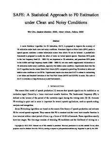
L(f ) = L (f |x1,2,...,K ) − Lcal (f )− (11) Z log exp[L− (f 0 |x1,2,...,K ) − Lcal (f 0 )]df 0 (12) The procedures above, from feature extraction to computing the normalized likelihood, are repeated at a fixed time interval. A likelihood map L(f, t) across time and frequency is generated (central plot in Fig. 3). To track the peak frequency in a robust manner, the likelihood map is first sampled on a log-spaced frequency grid and then passed into a Viterbi path searcher as the observation probability. The transition probability for the Viterbi search, which controls the range of F0 dynamics, is set according to a normal distribution in logfrequency domain with zero mean and a standard deviation of 2 octave/s. The resulting sequence of frequency indices is refined using parabolic interpolation on the likelihood map, in a way comparable to step 5 of YIN[5]. Finally, the F0 estimation algorithm gives a continuous log-F0 trajectory. The voicing status has yet to be determined, as explained in the following section.

300

600

900

1,200

1,500

time (frame) Fig. 3. From top to bottom: log p20 (f |x20 ) computed from a speech sample; estimated F0 trajectory superimposed on the log likelihood map; F0 likelihood and log voicing probability along the F0 trajectory. 4. VOICING DETECTION The F0 estimation stage outputs a F0 likelihood map across time and frequency. Over regions exhibiting strong periodicity, the F0 likelihood tends to be unimodal across frequency; over noisy or silent regions, the likelihood is generally flat, as illustrated in the central plot in Fig. 3. It thus comes naturally to interpret the peak F0 likelihood as an indication of voicing status. While a hard threshold on the peak likelihood or entropy can reasonably separate voiced and unvoiced speech, it is vulnerable to spurious likelihood fluctuations during unvoiced regions. In the direction of improving the robustness, instead of taking maxf L(f, t), we define the peak likelihood as L(f0 (t), t) so that the voicing decision to be made will be consistent with the F0 estimate. In addition, the peak likelihood is decoded by a two-state HMM, where the states map to voiced/unvoiced status, each paired with a scalar output distribution in the log likelihood space. An intriguing question at this point is to find out the distribution of the peak likelihood on unvoiced samples, that is, “a probability distribution of a probability mass or density”. Following the strategy of computing the calibration function Lcal , yet another Monte-Carlo simulation is performed on white noise input signals, from which peak F0 likelihood is extracted. It is empirically found that L(f0 (t), t) follows a normal distribution; on a grid-approximation of L(f, t) with

128 log-spaced frequency bins, the mean is −4.78 and the variance is 0.02. It is worth noting that the mean is close to but slightly greater than the log probability of a uniform dis1 = −4.852. tribution, log 128 The distribution of peak likelihood on voiced samples, however, cannot be determined through simulation as the SNR of voiced speech can vary depending on the environment and context. Assuming the distribution in question is also normal, we estimate the mean and variance from the peak likelihood data using Baum-Welch HMM training algorithm, starting with an initial mean of −2.0 and an initial variance of 1.0. The transition probability between voiced and unvoiced states is also estimated using Baum-Welch algorithm. 4.1. Tricks and Implementation Details Dithering. It is observed that the voicing detector is prone to picking up small sinusoidal interferences during silent and unvoiced regions. A simple workaround is to dither the input signal with a white noise at 2% the maximal amplitude. Smoothing of the likelihood map. The current design of IF and SNR estimators assumes quasi-stationary harmonic amplitude. Examination of the harmonic SNR estimated from speech signals shows that the amplitude modulation at vowel onsets and endings leads to an underestimated SNR. Such error affects the voicing decision in later stages of the algorithm, shortening each voiced region by 1 or 2 periods. To alleviate this problem, the F0 likelihood map is smoothed by a moving average filter prior to voicing detection, similar to the strategy adopted in the baseline method[4]. An important difference, however, is that Nebula uses a frequency-dependent moving average filter, ¯ t) = f L(f, 3

Z

t+1.5/f

L(f, t)dt

(13)

t−1.5/f

5. EVALUATION The proposed algorithm is tested on clean speech samples from CSTR[6] and CMU Arctic[7] databases. Criterion from Drugman, et al.[9] are adopted to assess the accuracy of F0 and voicing status estimation. Specifically, the F0 Frame Error (FFE) indicates the overall performance of an algorithm, which breaks down into the Gross Pitch Error (GPE) and Voicing Decision Error (VDE). The Gross Pitch Error is defined as the percentage of frames whose estimated F0 deviate from the ground truth by more than 20%, among all voiced frames with correct voicing decision. Datasets and the ground truth. The CSTR database contains 50 English sentences each from one male and one female speaker. The reference F0 and voicing labels included in the database are interpolated at a 5 ms interval to be used as the ground truth for this study. For CMU Arctic database, the first 50 sentences each from two male speakers (“jmk”

and “bdl”) and one female speaker (“slt”) are selected. The ground truth is extracted from EGG signals using Praat[8] with the default pitch tracking parameters, also at a 5 ms interval. Other methods involved in the testing. The following F0 and voicing estimation algorithms are compared against Nebula: YANGsaf[4], DIO[10], SAcC[3], RAPT[11], Praat[8] and SRH[9]. For all methods across all speakers, the search range for F0 is set to [55, 400] Hz while all other parameters remain at their default values. The results from SAcC and SRH, only available at a 10 ms interval, are interpolated to match the rate of the ground truth. Method Nebula RAPT Praat YANGsaf SAcC SRH DIO

FFE 5.53 (7.39) 5.96 (6.77) 6.35 (8.13) 7.33 (8.54) 7.63 (9.50) 8.28 (9.82) 9.08 (10.14)

GPE 0.30 (0.61) 0.74 (1.09) 0.57 (1.44) 1.14 (2.56) 0.67 (1.59) 0.71 (0.82) 0.54 (1.07)

VDE 5.39 (7.01) 5.61 (6.49) 6.10 (7.78) 6.75 (7.95) 7.29 (8.97) 7.98 (9.56) 8.81 (9.86)

Table 1. Table of average and worst-case scenario performance across all databases, ranked in ascending average FFE. Table 1 summarizes the results of the evaluation across all databases, including the average and worst-case1 (in parenthesis) error percentages of each algorithm being considered. It is seen that Nebula has a clear advantage over all criterion in terms of average performance. In the worst-case scenario, while RAPT outperforms Nebula on voicing detection by a 0.5% margin, Nebula remains being the second best overall. A major source of voicing detection errors is found to be the underestimated SNR at voiced/unvoiced boundaries, mentioned in section 4.1, even after frequency-dependent likelihood smoothing. It is also worth noting that Nebula reduces gross error rate to a negligible level. We believe such improvement over YANGsaf can be attributed to the inclusion of SNR2, IF2 and SNR0 feature extractors, under a carefully designed and calibrated probabilistic framework. 6. CONCLUSION We proposed Nebula, a F0 and voicing status estimation algorithm. Contributions of this study include: (1) a conditional GMM based framework combining F0 estimates from multiple features across multiple channels; (2) using synthetic data generated from Monte-Carlo simulations for model training; (3) extending the feature extraction system to reduce double and half-frequency errors; (4) a likelihood-based adaptive method for voicing detection. Future work should focus on improving the voicing detection and robustness against noise. 1 The worst-case percentage is defined as the minimum average performance across all speakers.

7. REFERENCES [1] K. Hua, “Improving YANGsaf F0 estimator with adaptive Kalman filter,” in Interspeech, Stockholm, 2017. [2] W. Chu and A. Alwan, “SAFE: A statistical approach to F0 estimation under clean and noisy conditions,” IEEE Transactions on Audio, Speech, and Language Processing, vol. 20, no. 3, pp. 933944, 2012. [3] B.S. Lee and D. Ellis, “Noise robust pitch tracking by subband autocorrelation classification,” in Interspeech, Portland, 2012. [4] H. Kawahara, Y. Agiomyrgiannakis, and H. Zen, “Using instantaneous frequency and aperiodicity detection to estimate F0 for high-quality speech synthesis,” in 9th ISCA Workshop on Speech Synthesis, Sunnyvale, 2016. [5] A. de Cheveigne and H. Kawahara, “YIN, a fundamental frequency estimator for speech and music,” The Journal of the Acoustical Society of America, vol. 111, no. 4, p. 1917, 2002. [6] P. C. Bagshaw, S. M. Hiller and M. A. Jack, “Enhanced pitch tracking and the processing of f0 contours for computer aided intonation teaching,” in Eurospeech, Berlin, 1993. [7] J. Kominek and A. W. Black, “The CMU Arctic speech databases,” in Fifth ISCA Workshop on Speech Synthesis, Pittsburgh, 2004. [8] P. Boersma and D. Weenink, “Praat: doing phonetics by computer,” Version 6.0.22, retrieved 15 November 2016 from http://www.praat.org/. 2016. [Computer program] [9] T. Drugman and A. Alwan. “Joint robust voicing detection and pitch estimation based on residual harmonics,” in Interspeech, Florence, 2011. [10] M. Morise, H. Kawahara, and T. Nishiura. “Rapid F0 estimation for high-SNR speech based on fundamental component extraction,” Trans. IEICEJ, vol. J93-d, no. 2, pp. 109117, 2010, [in Japanese]. [11] D. Talkin, “A robust algorithm for pitch tracking (RAPT),” Speech coding and synthesis, vol. 495, p. 518, 1995.