BIOCHEMICAL TRANSPORT MODELING, ESTIMATION AND DETECTION IN REALISTIC ENVIRONMENTS Mathias Ortner† and Arye Nehorai†∗ December 6, 2008
Contents 1 Introduction
2
2 Physical and statistical models 2.1 Assumptions . . . . . . . . . . . . . . . . . . . . . . . . . . . 2.2 Physical dispersion model . . . . . . . . . . . . . . . . . . . . 2.2.1 Advective model . . . . . . . . . . . . . . . . . . . . . 2.2.2 Boundary conditions . . . . . . . . . . . . . . . . . . . 2.2.3 Initial substance distribution and sources . . . . . . . 2.3 Measurement model . . . . . . . . . . . . . . . . . . . . . . . 2.3.1 Fluid simulations, transport model and inclusion of random effects . . . . . . . . . . . . . . . . . . . . . .
4 4 5 5 6 6 6
3 Transport modeling using Monte Carlo approximation 3.1 Stochastic diffusion . . . . . . . . . . . . . . . . . . . . . . 3.1.1 Diffusion equation . . . . . . . . . . . . . . . . . . 3.1.2 Stochastic process . . . . . . . . . . . . . . . . . . 3.1.3 Feynman-Kac formula . . . . . . . . . . . . . . . . 3.1.4 Boundary conditions . . . . . . . . . . . . . . . . . ∗†
. . . . .
. . . . .
7 8 8 9 9 10 10
A. Nehorai is with Washington University in Saint Louis. Emails:
[email protected] and
[email protected]. Adress: Department of Electrical and Systems Engineering Campus Box 1127 Washington University in St. Louis St. Louis, MO 63130 USA. Tel: 314-935-7520. Fax: 314-935-7500
1
3.1.5 3.2 3.3
Approximated stochastic diffusion surements . . . . . . . . . . . . . . Simulation and convergence . . . . . . . . Application to the transport problem . . . 3.3.1 Stochastic transport model . . . . 3.3.2 Monte Carlo approximations . . . 3.3.3 Unit response . . . . . . . . . . . . 3.3.4 Likelihood . . . . . . . . . . . . . . 3.3.5 Wind turbulence modeling . . . .
4 Localizing the source(s) 4.1 Inverse problem and random field 4.1.1 Bayesian model . . . . . . 4.2 Algorithm . . . . . . . . . . . . . 4.3 Results . . . . . . . . . . . . . . .
and . . . . . . . . . . . . . . . . . . . . . . . .
sensor . . . . . . . . . . . . . . . . . . . . . . . . . . . . . . . .
mea. . . . . . . . . . . . . . . . . . . . . . . . . . . . . . . .
11 12 14 14 15 15 16 16
. . . .
. . . .
. . . .
. . . .
. . . .
. . . .
. . . .
. . . .
. . . .
. . . .
. . . .
. . . .
. . . .
18 18 19 20 20
5 Sequential Detection 5.1 Discussion . . . . . . . . . . . . . . . . . 5.2 A sequential detector . . . . . . . . . . . 5.2.1 Sufficient statistics . . . . . . . . 5.2.2 Resulting tests . . . . . . . . . . 5.3 Threshold and false alarm rate . . . . . 5.3.1 Average run length . . . . . . . . 5.4 Performance . . . . . . . . . . . . . . . . 5.4.1 Probability of detection . . . . . 5.4.2 Minimum signal level . . . . . . 5.4.3 Expected delay before detection 5.5 Simulations . . . . . . . . . . . . . . . . 5.5.1 Online detection . . . . . . . . . 5.5.2 Performance measures . . . . . .
. . . . . . . . . . . . .
. . . . . . . . . . . . .
. . . . . . . . . . . . .
. . . . . . . . . . . . .
. . . . . . . . . . . . .
. . . . . . . . . . . . .
. . . . . . . . . . . . .
. . . . . . . . . . . . .
. . . . . . . . . . . . .
. . . . . . . . . . . . .
. . . . . . . . . . . . .
. . . . . . . . . . . . .
21 21 22 22 23 23 23 24 24 24 25 25 25 25
6 Conclusion
1
. . . .
. . . .
. . . .
26
Introduction
A new numerical approach. We present1 in this chapter a new approach for computing and using a numerical forward physical dispersion model relating the source to the measurements given by an array of biochemical 1
We orginally presented this work in [1] and [2].
2
sensors in realistic environments. The approach presented here provides a modeling framework that accounts for complex geometries and allows full use of software-simulated random wind turbulence. The key point of our approach is that we decouple the “fluid simulation” part from the “transport compution”. In particular we show on a simple but realistic example how to incorporate numerical simulations including random effects. The approach we propose is generic enough to incorporate additional random effects, including chemical reactions, temperature effects, and radioactive decaying. The Monte Carlo approach we employ is based on a Feynman-Kac representation, and therefore does not require solving the problem on the entire domain, but only at the sensor positions. The required computational time is thereby limited. Illustrating example : monitoring biochemical events. We take monitoring biological or chemical events as an illustrating example. The prospect of a biological or chemical attack is a prominent security issue. Release in a closed space such as subways or buildings could result in especially high doses and impact [3]-[5]. In our previous work, we presented detection and estimation techniques for simple scenarios where analytical solutions to the transport equations are available (see [6]-[10]). In [11] we considered numerical solutions given by finite elements methods. Refer to [12]-[17] for additional work on the subject, including ways of considering the impact of turbulence on urban diffusion. Inverse problem. Localization of the source is important in order to predict the cloud propagation in space and time and consequently make quick emergency decisions. We consider cases involving multiple sources and propose to use a generic Bayesian approach to solve the inverse problem based on a suitable prior model. This framework allows us to consider multiple sources with unknown initial diffusion times and release intensities. The estimator we consider is the a posteriori probability distribution of the source locations, with a major consequence: in the case of uncertainties due to a lack of measurements or the presence of several diffusive sources, the computed a posteriori distribution shows all relevant hypotheses. Detection framework. We propose a sequential detector. The difficulty of the detection task arises from the unknown parameters. As in real applications the starting time of the spread and the original concentration and location of the initial delivery are unknown, we propose using a sequential 3
generalized likelihood ratio test (GLRT) as advocated in [33]. Such a detector relies on setting a threshold usually fixed by deciding on the average time before a false alarm. We propose in this chapter a bound on this average time and show that the bound is a good approximation using numerical examples. Chapter Organization. This chapter is organized as follows: in Section 2 we detail the physical dispersion model and present the measurement model. In Section 3 we present the setup for numerical approximations of the dispersion through Monte Carlo simulations of the associated stochastic diffusion, assuming known arbitrary geometry. We also propose an ad-hoc approach to account for stochastic wind turbulence based on the result of numerical fluid computations. In Section 4 we explain the Bayesian model employed for localizing several sources and detail the Metropolis-Hastings algorithm used to sample the posterior density. The results from Sections 3 and 4 are illustrated by a toy example representing an urban environment. In Section 5 we develop the sequential detector. In Section 5.3, we analyze the false alarm behavior and propose a bound based on geometric considerations. In Section 5.4, we detail how performance measures such as the probability of detection can be computed.
2
Physical and statistical models
In this section we discuss the physical model we use to describe the dispersion of a chemical substance in a fluid. We employ the framework provided by [7, 10]. We also detail the statistical sensor measurement model. The goal is to determine a numerical relationship between the contaminant sources and sensor measurements.
2.1
Assumptions
We assume the geometry of the setup to be known, including the locations of the biochemical sensors and boundaries of the problem (the building geometries in the case of urban environments). We also assume a knowledge of the wind distribution in the considered setup. For instance, in the presented examples we assume that the wind has a known main direction and we suppose the availability of software that is capable of computing the resulting wind distribution over the area, including vorticities for modeling turbulent effects. We assume also that we know the diffusion properties of the con-
4
Figure 1: An example of a dispersion scenario: an urban environment (135 m by 225 m) modeled by a set of rectangles. Wind is shown to come from the north at a speed of 54 km/h. The rectangles stand for buildings. Six sensors (shown as circles) are placed in the area, and a chemical substance is instantaneously released at two points (shown as disks). taminant (diffusion coefficient) and that the sensors have been calibrated, resulting in a known noise variance. Figure 1 shows a toy example illustrating an urban environment that is modeled by a set of rectangles with two release sources and six sensors. Note that the setup in the figure is considered two-dimensional (2D) for computational simplicity, although the framework described in the rest of this section is presented in three dimensions (3D).
2.2 2.2.1
Physical dispersion model Advective model
We consider a bounded open domain D ⊂ R3 . Let r = (x, y, z) be a point in D. Denote by c(r, t) the dispersive substance concentration at a point r and time t. The transport equation in the presence of a wind field v(r, t) ∈ R3 is given by the following equation [6] when the medium is assumed to be incompressible (div(v) = 0), ∂c = div(K∇c) − ∇c · v ∂t 5
(1)
where K is a 3 × 3 matrix of conduction (or diffusivity). We suppose that K is a function of the space variables. To consider realistic scenarios, we need to use a wind field that includes turbulent effects resulting in either random or time dependent wind fields v. We discuss this point in more detail in Section 2.3.1. Figure 2 presents a diffusion simulation on the example presented in Figure 1. t=0.0
t=0.5
t=1.0
t=1.5
t=3.5
Figure 2: Simulated diffusion of a contaminant at different time instants computed by dedicated software [19] that includes realistic turbulence computations. The gray level corresponds to the concentration of a contaminant.
2.2.2
Boundary conditions
Let ∂D be the boundaries of the domain D. We assume [1] two kinds of domain boundary conditions and divide ∂D into two disjoint subsets denoted by ∂DN and ∂DD corresponding to Neumann and Dirichlet conditions. The former means ∇c(r) · n(r) = 0, for all r ∈ ∂DN and the latter c(r) = 0, for all r ∈ ∂DD , where n(r) is the normal vector at any point r belonging to ∂D. Neumann conditions describe boundaries that do not affect the substance concentration, while Dirichlet conditions correspond to boundaries within the domain D and the “outside world”. 2.2.3
Initial substance distribution and sources
We assume that the sources have released a certain amount of a substance into the environment when the diffusion begins (instantaneous sources) and denote by c0 (r) the substance concentration at time t = 0 (release time). This formulation covers most of the usual cases [1], due to the linearity of the advection-diffusion equation.
2.3
Measurement model
To model the measurements, we suppose a spatially distributed array of m biochemical sensors located at known positions r1 , . . . , rm . We assume that 6
each sensor takes measurements at times t0 , . . . , tn . Referring to our earlier work [7], we adopt the following measurement model: y(ri , tj ) = c(ri , tj ) + ²i,j ,
² ∼ N (0, σe2 ),
i = 1, . . . , m
j = 0, . . . , n (2)
where ² represents measurement noise and modeling errors. In the remainder of this paper, we assume that σe is known from a calibration step. 2.3.1
Fluid simulations, transport model and inclusion of random effects
A major modeling issue in Equation (1) is the assumed knowledge of the transport term v due to the wind. The wind actually is a function of both the position and time variables. In urban areas, as shown in [21], random effects generated by wind turbulence may have a huge impact on the dispersal behavior of the biochemical contaminant. Precise knowledge of this variable is impossible to obtain even if many wind sensors are available owing to the chaotic nature of the wind. One way to model the chaotic nature of turbulence is to use a deterministic representation of the wind describing the ergodic effect of random turbulence. Eddy diffusivities that approximate the turbulent effect by a higher diffusion coefficient [22] are a first possible model. Another idea is to use Reynolds decomposition v = v ¯ + ξ and consider random fluctuations of the wind around the mean [20]. We proposed in our paper [1] a different approach, one that allows us to include more realistic wind descriptions for specific scenarios based on wind computation provided by a dedicated software [19]. For instance, in the outdoor problem of Figure 1, we suppose that the wind comes from a main direction. We then employ the flow solver to compute the wind distribution over space and time. Figure 3 shows some samples of the obtained wind field at different times using this software. In our case, we use the default values provided by the Gerris flow solver. For the scenario of Figure 1 (135 m by 225 m) we assume that the wind is coming from the north at a speed of 54km/h. It results in a mean wind field of 2 km/h horizontally and 62 km/h vertically. The average standard deviation obtained is 60 km/h horizontally and 80 km/h vertically. The numerical forward computation technique we propose allows making full use of these snapshots as detailed in Section 3.3.5.
7
t=0.0
t=3.5
t=7.0
t=11.0
t=14.5
vx
vy
Figure 3: Temporal snapshots of wind distribution at different times given by dedicated software [19] using the scenario presented in Figure 1, with a wind value of 35 km/h. Top: x component, bottom: y component.
3
Transport modeling using Monte Carlo approximation
In this section we propose a numerical approach to solve the transport equation (1) in the presence of turbulence. The proposed approach is generic and uses random walks to compute the solution of a diffusion equation at a precise location and time. The interesting point is that these random walks are started from the point of interest (e.g. the sensor) and go backward in time with respect to the physical interpretation of the diffusion equation. As a consequence, the problem is only solved at the important locations (sensor positions), saving computational time. Of course, the random walks depend on the considered diffusion equation and boundary conditions. For simplicity, in the remainder of this section we will consider a one dimensional (1D) setup. Extensions to 2D or 3D frameworks are straightforward. Note that in order to present a generic framework, we use specific notations and replace the concentration function c by u.
3.1
Stochastic diffusion
We present here the general mathematical link between diffusion equations and their associated stochastic process. This link can be seen as the relationship between the macro- and the microscopic descriptions of the physical 8
phenomena. 3.1.1
Diffusion equation
Consider the following general diffusion operator G acting on a function u(x, t): 1 du d2 u Gu = σ 2 (x) 2 + b(x) . (3) 2 dx dx We are interested in solving the diffusion equation: du = Gu − Ku , dt
u(x, 0) = u0 (x)
(4)
where K is a real-valued function that might depend on the variable location x. In the case of the heat equation, K(x) stands for an additional cooling or heating effect at x. In our biochemical case, the variable of interest is the concentration (u = c). The transport term b(x) then describes the wind effect (b = −v),√whereas the diffusion term σ represents the chemical diffusion effect (σ = 2K). In the case of the chemical diffusion, −Ku is a source/sink term that represents radioactive decaying, chemical reaction or incorporate a divergence term for compressible fluids. For the sake of simplicity we assume that the fluid is incompressible K = 0, although the framework can be applied similarly for non null K. 3.1.2
Stochastic process
We introduce the following stochastic diffusion process in the Ito sense to represent the microscopic description of Equation (4). As we will detail, this process can be seen as the evolution equation of individual particles going backward with respect to the real physical phenomena. We consider Xt given by: X0 = x 0 (5) dXt = b(Xt )dt + σ(Xt )dWt where Wt represents a Brownian motion. The position value of Xt at time t has a probability distribution Px0 ,t (Xt ∈ ·) that depends on the initial location x0 and time t. We use Ex0 ,t [·] to denote the corresponding expectation family. The relationship between this stochastic process and the diffusion problem described by Equations (4) and (3) arises from the property described below in Equation (6).
9
3.1.3
Feynman-Kac formula
The Feynman-Kac formula relates the continuous macroscopic transport description (4) to the stochastic microscopic equation (5) through the following property. Under certain regularity conditions on σ(·) and b(·), the following function is a solution to the diffusion problem (4): · µ Z t ¶ ¸ u(x0 , t) = Ex0 ,t exp − K(Xτ )dτ u0 (Xt ) . 0
In the case of K = 0 (incompressible flow), we obtain: u(x0 , t) = Ex0 ,t [u0 (Xt )].
(6)
For a given initial condition x → u0 (x), replacing x0 , t by a sensor coordinates xs , ts (sensor position and sample time), the Feynman-Kac formula (6) asserts that the value of the solution u(xs , ts ) at a given location xs and time ts is given by the expectation of the initial condition Exs ,ts [u0 (Xts )]. This expectation uses the probability distribution Pxs ,ts (Xts ∈ ·) of Xts , the location of the process (Xt ) starting from xs after time ts . The important point is that the stochastic process is started from the sensor location xs : the formula reflects a backward property compared with usual forward computation methods going from the source to the sensor. In our application the transport term b is given by b = −v (see Equations (3) and (4)). The process is accordingly drifted by the opposite of the wind and goes backward with respect to the real physical transport phenomena. Another interesting point is that the random walk is independent of the initial condition: one can compute the solutions associated with different initial conditions by using the same set of random walk samples. We present in Figure 4 an illustration of the Feynman-Kac property. Suppose that the initial condition is given by an indicator function u0 (x) = 1(x ∈ A). The Feynman-Kac formula states that u(xs , ts ) = Pxs ,ts (Xts ∈ A), i.e. that the solution value u at xs and time ts is given by the probability that the process Xt starting from xs hits the set A after time ts . Thus, to obtain the solution of the heat equation at a particular location and time, one can launch random walks starting from this point and compute the empirical probability of hitting the set A after the considered time. 3.1.4
Boundary conditions
The behavior of the stochastic process depends on the boundary conditions. For Dirichlet boundaries, the process can be killed, or stopped. For Neumann conditions, the process can be reflected and for mixed conditions more 10
source
sensor
A
random walks
diffusion result
A
t=ts
t=0
Figure 4: Illustration of the Feynman-Kac formula (6). Left: the initial condition (t = 0) is given by the indicator function of set A, i.e. u0 (x) = 1(x ∈ A). The disk represents A, the circle shows the sensor location xs . Middle: illustration of the analytical result of a heat equation at t = ts . Right, realizations of the stochastic process starting from the sensor location xs . According to the Feynman-Kac formula, the result of the diffusion in xs after time ts is given by the probability that the random walks of the last image hit the set A : u(xs , ts ) = P(Xts ∈ A). generic Feynman-Kac representations need to be considered [23]. We present later how to handle Dirichlet and Neumann conditons. 3.1.5
Approximated stochastic diffusion and sensor measurements
To implement the Feynman-Kac formula in practice we need to consider simulations of the process (Xt ). More specifically, we need to simulate the random process (Xt ) starting from x and then compute the empirical expectation associated with Equation (6). After collecting N samples Xt1 , . . . , XtN of the process location at time t, we calculate a natural estimate of u(x, t) by: PN u0 (Xti ) . (7) u ˆ(x, t)u0 = i=1 N This result demonstrates a direct relationship between the solution at a fixed position and a given time (x, t) and the initial condition x → u0 (x). ˆ(x, t)u0 can Once a sample (Xt1 , . . . , XtN ) has been obtained, the solution u be computed for different functions x → u0 (x) using Equation (7) without requiring further generation of new samples. In the context of locating a chemical source using an array of m sensors, 11
we need to launch N random walks starting from each of the m sensors in order to obtain the concentration evolution at each of the sensor locations. The first advantage of the proposed approach to solve the forward problem over other classical numerical tools like finite element methods is that it allows a stochastic modeling of the wind. Second, this method is highly suitable for parallel computing: the random walks are independent and can be therefore generated by different computers. Another advantage is that this approach computes the solution only at specific points and time of interest and does not try to solve the entire problem. As a consequence, even when we consider a large setup (a real city, for instance), the processing load evolves linearly with the number of sensors and the considered diffusion duration. The major drawback is the needed computational time: the method is more computationally intensive in small setups than finite elements (in practice, we use N = 10000 or N = 50000). However, as already stated, the approach is particularly useful for large setups, in terms of domain size and dimension. Another point is that the forward simulation can be done ahead of time as we show it in Section 3.3.2.
3.2
Simulation and convergence
We now focus on the simulations of the stochastic process involved in Equation (5). The discretization of a stochastic process is a research field in itself and has been the subject of a huge body of literature, especially in the past ten years (see for instance [24]). Depending on the type of process to be approximated, convergence results may exist or not. In our case, the infinitesimal generator is very simple (it essentially corresponds to the heat equation), and one can expect some nice convergence results. However, the boundary conditions complicate the problem. In this framework, we use a reflected stochastic diffusion to model the Neumann boundary conditions. Different schemes have been proposed (e.g. by Lepingle [25] or by Costantini et al. [23]). The weak convergence of the approach we use has been proved only recently by Bossy, Godet, and Talay [26]. We detail later the simulation procedure for the case of the Neumann boundary conditions, while restricting the presentation here to the simple case of infinite domains without boundaries. Infinite domain: In the case of an infinite domain D (without any boundary conditions), the following Euler scheme is known to converge in the weak sense [24]. Define a time discretization parameter h giving the associated discrete times tk = hk ∈ [0, T ], where k is an integer. Sampling the process described in Equation (5) is straightforward and is obtained by the following 12
iterative procedure: X0h Xthk+1
= x0 = Xthk + b(Xthk )h + σ(Xthk )(Wtk+1 − Wtk )
(8)
where Wtk+1 − Wtk is simulated by a Gaussian random variable with mean 0 and variance h. The weak error E[f (XTh )] − E[f (XT )] for f in a class of smooth functions can be expanded in terms of powers of h, provided some regularity conditions on f or some conditions on X are satisfied [26]. Neumann conditions: In the case of an open bounded domain D, the scheme presented here needs to be adapted. The weak convergence of the following algorithm has been recently provided by Bossy, Godet, and Talay [26]. This algorithm is based on symmetric reflections of the random walk against the boundaries. X0h = x, ¯ For Xthk ∈ D, h 1 Ytk+1 = Xthk + b(Xthk )h + σ(Xthk )(Wtk+1 − Wtk ) ½ γ ¯ S∂D (Ythk+1 ) if Ythk+1 6∈ D h 2 Xtk+1 = h Xtk+1 otherwise.
(9)
γ Here S∂D (x) represents the mirror point of the point x with respect to the boundary ∂D taken using the γ direction. The vector γ depends on the boundary condition: ∇u(t, x) · γ = 0 for (t, x) ∈ [0, T ] × ∂D. In our case γ(x) = n(x), resulting in a symmetric reflection (see Figure 5). In order to be consistent, this definition supposes that there are no ambiguities on the border on which to reflect (h thus needs to be small enough). When ¯ one can a bad case is encountered (the symmetric point lies outside of D), h re-simulate Ytk+1 . Note that according to [26], the probability of such events goes exponentially to zero with h. Through conditions on the smoothness of D, ∂D, b, and σ, Bossy, Godet, and Talay have shown the following result: for f smooth enough (see the original paper) and compatible with the problem:
|E[f (XTh )] − E[f (XT )]| ≤ const(T )C(f )h where const is uniform in x and f , and C(f ) depends on the sum of ∞ norm of the differential of f until order 5 (see [26] for details.)
13
11 00 11 00
Figure 5: Illustration of Neumann and Dirichlet boundaries. Left: trajectory of a reflected process illustrating the numerical scheme used to account for Neumann boundary conditions. In gray, the originally proposed point replaced by its mirror point with respect to the boundary. Right: trajectory of an absorbed realization illustrating the effect of a Dirichlet boundary. Dirichlet conditions: The simplest way [32], to account for Dirichlet boundaries, is to stop the random walk when it hits such a boundary. The Feynman-Kac formula then becomes u(x, t) = Ex [u0 (Xt )1(t < τ )], τ being the stopping time associated with the event: “Xt crosses a Dirichlet boundary.” Note that we denote by 1 the indicator function.
3.3
Application to the transport problem
We present here the numerical method for implementing the particular case of our transport problem (1). We also present its consequences on the likelihood of the measurements. We propose a way to include turbulent flow within the computations. 3.3.1
Stochastic transport model
By identifying the generic diffusion Equation (4) with the transport equation (1), we obtain, in 2D or 3D: √ b(r) = −v, σ = 2K where we used the square root for a definite positive matrix. Note again that the wind is reversed: the Feynman-Kac formula works in a backward mode as discussed earlier. The discrete scheme in Equation (8) results in the following iterations: q Xhtk+1 = Xhtk − v(Xhtk )h + 2K(Xhtk )(Wtk+1 − Wtk ) (10) 14
where Wtk+1 −Wtk is obtained by the generation of two or three (depending on the dimension) independent and identically distributed normal variables, with mean 0 and variance h. In practice we consider an isotropic and homogeneous matrix and the square root correspond to the scalar one. 3.3.2
Monte Carlo approximations
To obtain a handy version of the empirical distribution of the particles after time h, we use a discrete version of the domain D. Denote by Λ a set of sites in D associated with a grid of points indexed by z and |Λ| = card(Λ) the number of elements in Λ. We partition D into small squares ∆D(z) (pixel like): [ D= ∆D(z) and ∆D(z) ∩ ∆D(z 0 ) = ∅, ∀z 6= z 0 z∈Λ
For given sensor location and time (ri , tj ), diffusion matrix K, and wind distribution v, the Monte Carlo simulations give N final points, denoted by Xr1i ,tj , . . . , XrNi ,tj . Let pi,j,z be the average number of such points falling in the element ∆D(z): pi,j,z =
N 1 X 1(Xrki ,tj ∈ ∆D(z)). N k=1
For a given initial concentration value function r → c0 (r), the Feynman-Kac formula (6) yields: X ci,j = pi,j,z c0 (z) (11) z∈Λ
where ci,j is the calculated estimate of the concentration at the location ri and time tj . We present two results of the computations of these transport probabilities pi,j,z on Figure 6. For a given sensor (i = 1, bottom left on Figure 1) we illustrate the probabilities pi,j,z for different times tj . The figure illustrates the notion of backward evolution, the p1,j,z indeed standing for the probability that a particle arriving at the first sensor was launched from a site z at a time tj earlier. 3.3.3
Unit response
Consider a time discretization parameter δt and regularly spaced discrete times (t0 , . . . , tj , . . .) = (0, . . . , jδt , . . .). The sequence (pi,j,z )0≤j≤n can be seen as the unit response of the sensor located at ri to a unit instantaneous 15
t=0.0
t=1.5
t=3.0
t=4.5
t=6.0
t=7.5
t=8.0
t=9.5
t=12.0
t=14.5
Figure 6: Illustration of the pi,j,z for i = 1 (bottom left sensor in Figure 1) and several successive times tj . The mapping z → pi,j,z corresponds to the empirical probability density of the origin z of a particle arriving at the ith sensor after a time tj . In each image, the higher pi,j,z the darker the corresponding pixel. The gray scale is adapted for each image, resulting in the overall darkening. substance release at the site indexed by z. In the remainder of this article, we will consider δt = 1 and denote by t ∈ {0, . . . , n} the time index for the impulse response (see Equation (12)). 3.3.4
Likelihood
Denote by Y all the measurements yi,t lumped into a single mn dimensioned vector. Let C be the vector of all initial concentration c0 (z) in every point z ∈ Λ. By assuming independent measurements and a Gaussian noise, equation (11) yields the likelihood f (Y/σe , C): Ã !2 m n−1 X X X 1 1 f= √ exp − 2 yi,t − pi,t,z c0 (z) . (12) 2σe ( 2πσe )mn i=1 t=0 z∈Λ 3.3.5
Wind turbulence modeling
We present here an ad-hoc procedure to account for wind turbulence. To illustrate the procedure, we focus on the urban environment example presented in Figure 1. We compute a solution to the Navier Stokes equation for the wind distribution using a dedicated program called Gerris [19]. This 16
computation is made possible because of the assumption that the wind in this example is mainly coming from the north. We then obtain several snapshots of the wind distribution such as those shown in Figure 3. A common way to account for turbulence is to use a mean wind field [21], averaging the obtained snapshots. However, our preliminary results indicated that using a mean field would be inappropriate especially for outdoor applications. For instance, at a location where the turbulence is large, the average wind can be null if the wind direction variability is large enough. Another solution is to decompose the wind into a mean field and a Gaussian random variable [20]. However, even if the turbulence values are chaotic in time, there is a strong spatial correlation between neighboring points. Supposing independence between neighboring points might therefore be incoherent while estimating the correlation might not be a simple issue. We now propose a simple way of incorporating turbulent flow behavior in the computations of the random walks. We take advantage of the stochastic formulation of the numerical computations we proposed in this section. Let {v1 , · · · , vl } be l spatial snapshots of the wind distribution over the whole setup, provided by a software. For instance, we use [19] to compute 30 of such snapshots under the constant main wind direction assumption. We propose to replace the wind drift v in Equation (10) by one snapshot randomly selected among {v1 , · · · , vl }. In order to account for the variability of the turbulent flow, we randomly change the snapshot used during the stochastic random walk (5). Each snapshot is used during a random time ν generated according to an exponential distribution with mean λ: ½ λeλν ν ≥ 0 ν ∼ fexp (ν; λ) = (13) 0 ν≥0 and once this random duration has expired, we uniformly select a new snapshot of the wind among the l possible snapshots before generating a new random duration and iterating the process. The parameter λ can be seen as the expected duration of a turbulence flurry, in practice we took λ = 1s. During a random walk of duration T , we use approximatively T /λ different snapshots. The first advantage of this approach comes from the implicitly modeled spatial correlation. The second advantage is that even if turbulence has a null average at one location, we still can account for large wind values. We present a result in Figure 7. On top, we show the transport probabilities pi,t,z computed using a mean wind field approximation. The results show that the main direction of the wind is taken into account, since the cloud of possible original locations goes towards the north with time. However, the bottom result obtained using our approach shows that using 17
t=0.0
t=1.5
t=3.0
t=5.0
t=7.0
t=0.0
t=1.5
t=3.0
t=5.0
t=7.0
Figure 7: Comparison of the effect of a mean wind field (top) and the proposed stochastic wind approach (bottom) on the transport probabilities pi,j,z . We present the transport probabilities associated with the second sensor (bottom center, in Figure 1). Top: results obtained using a mean wind field obtained using dedicated software [19]. Bottom: results obtained using our stochastic wind modeling which appears to increase the dispersive effect. randomly selected snapshots of the wind increases the predicted diffusivity, a result that is in line with the eddy diffusivity framework [22].
4
Localizing the source(s)
We describe briefly in this section the Bayesian approach we employed [1] for inferring the source location from the measurements. This task is useful for predicting the cloud evolution in space and time dispersion by applying the transport model to the estimated source(s) location(s).
4.1
Inverse problem and random field
We develop in this section a setup to introduce a Bayesian regularization term for solving the inverse problem. This Bayesian term allows us to consider distributed and therefore multiple sources. Additionally, the unknown initial time can be considered as a model parameter and to be estimated from the measurements.
18
4.1.1
Bayesian model
Likelihood: We consider a set of sites Λ and associate with each site an unknown initial concentration value c0 (z) = µz . The purpose of the source localization is to estimate the initial values µz using a set of measurements {y t0 , . . . , y n }. In the following, we assume that t0 , the initial release time, is approximatively known from a detection process. The likelihood of the measurements being given the set of values (µz )z∈Λ is then given by: Ã !2 m n−1 X X X 1 1 f (y/σe , (µz )z∈Λ ) = √ exp − 2 yi,t0 +t − pi,t,z µz . 2σe ( 2πσe )mn i=1 t=0
z∈Λ
(14) Prior model: We use the following mixture as a prior model for the (µz ). We state that µz should be equal to 0 with a probability 1 − ρ and uniformly distributed in [cmin , cmax ] with a probability ρ. The prior term can therefore be written as: X fprior ((µz )z∈Λ /ρ) = (1 − ρ)1[µz = 0] + ρ1[µz > 0 , µz ∈ [cmin , cmax ]]. z∈Λ
(15) The mixing parameter ρ should be chosen according to the size of the domain D and the number of sites |Λ|. A way to choose ρ is to make a prior decision about the average surface of the release. In practice we took ρ = 0.01, meaning that we state that the source surface is expected to be 1% of the overall domain area. Posterior density: The likelihood of the measurements, the prior model, and Bayes formula result in the following a posteriori distribution: ¢ ¡ fpost (µ)z∈Λ /y t0 , . . . , y n , σe , ρ, t0 µ = ¶ Pm Pn−1 P 2 ¡ ¢− q µz pi,t,z −yi,t+t0 ) ( C 2πσe2 2 ((1 − ρ)Υ + ρΨ) exp − i=1 t=0 z∈Λ 2σ 2 e
(16) where Υ = card{z ∈ Λ : µz = 0} and Ψ = card{s ∈ Λ : µz > 0}, and C is the normalizing constant. Note that according to the Bayes formula, C is the inverse R of the expectation of the likelihood under the prior model −1 C = B = f (y/µ)fprior (µ)dµ. The value of B is usually called the Bayesian Evidence [28] and can be used for model selection.
19
Estimator: For each site we consider the following two values: Ppost (µz > 0),
Epost (µz |µz > 0).
(17)
These estimators respectively correspond to the posterior probability of having a source at the location z, and the posterior conditional expectation of the source concentration, knowing that there is a source. The former provides the probability that there was a source at each location, whereas the latter gives the estimated intensity in that case. Estimating the initial time of release: Equation (16) assumes that the initial time of the transport phenomena is exactly known. However, this will hardly be the case, and we propose for estimating this unknown initial time to compute the Bayesian Evidence (C −1 , in Equation (16)) for several time hypotheses and then consider the maximum obtained value.
4.2
Algorithm
We employ [1] a Monte Carlo Markov chain method to sample the posterior distribution, and more precisely a Metropolis Hastings approach. This kind of sampler is especially suitable for our case, since we do not know the normalizing constant C in Equation (16). Note that C is actually another value we want to compute, since it provides the Bayesian evidence.
4.3
Results
We present in Figure 8 the result of the sampler. On the left, we show the posterior probability of having a source in each considered location (note that the gray-scale is logarithmic). The true locations of the sources were correctly found. On the right we show the a posteriori expectation of the initial intensity in each location conditioned by the event that there is a release. Note that in the locations were the probability of having a source is high, the estimated intensity is close to the real value (we recall that we used an initial intensity c0 = 5). For that particular example, we assumed the initial time to be known (t = t0 ). In the following section, we provide a result using the Bayesian evidence, for selecting a relevant initial time hypothesis. These results show that the random field approach is powerful for finding several sources.
20
0.25
1 0.9
0.2
0.8 0.7
0.15
0.6 0.5
0.1
0.4 0.3
0.05
0.2 0.1 0
0
Figure 8: Results of the source localization estimation given by the Bayesian approach. Left: Ppost (µz > 0), the probability of having a source in each location (logarithmic scale); right: Epost (µz |µz > 0), the average source intensity conditioned on the presence of a source. Note that the real initial concentration level used was c0 = 5. The result on the left provides for each location the probability that a source was present. The result on the right provides the estimated intensity in the case there was a source.
5
Sequential Detection
In this section we describe a framework [2] for detecting a biochemical release using the incoming measurements. The goal is to be able to detect a release as soon as possible.
5.1
Discussion
In sequential analysis, the measurements are considered as an incoming flow, and the goal is to select the hypothesis of interest as soon as possible. In our case, designing such a detector is of the utmost importance since we would like to assess the presence of a dispersive contaminant in a fluid with the smallest possible delay. For a detailed review of sequential detection, see Lai [34]. The problem of detecting a biochemical attack is complicated by the fact that the starting time is unknown. As a result, we need to focus on sequential change detection, which deals with the problem of detecting an abrupt change in the distribution of measurements. This topic has been actively researched in the last decades, both in theory [34, 35, 36] and for different applications, including target detection [37] as well as Internet security [38]. 21
Fundamental work on change-point detection has been done by Girshik and Rubin [39], Page [40], Roberts [41], and Shiryaev [42]. The two major competitive procedures mostly used today are the Shiryaev-Roberts-GirshikRubin [43] algorithm and Page’s cumulative sum (CUSUM) algorithm [44]. Both are known to be optimal when the observations are independent and identically distributed (i.i.d.) in pre-change and post-change distribution. In our chemical setup, although the change-point detection framework fits our goal well, the usual change-point detectors face some limitations, since we do not know the location of the hypothetical release nor its initial concentration. Moreover, the successive measurements are independent but not identically distributed, making analytical results hard to provide.
5.2
A sequential detector
In detection theory, a natural idea when dealing with unknown parameters is to use the likelihood of the best hypothesis under each assumption [45] resulting in GLRT. We consider three unknown parameters: the initial time δ, the location s ∈ Λ, and the intensity µ of an impulse substance source. We assume that the variance σe of the noise is known through a calibration step. Let yt = (y1,t , . . . , ym,t )T be the vector of m measurements given by the m sensors at time t. We then obtain the following sequential generalized likelihood ratio 1 (y , . . . , y ) fs,µ n δ 0 µ≥0 f (yδ , . . . , yn )
˜ n (y0 , . . . , yn ) = max max sup L 0≤δ≤n s∈Λ
(18)
Denoting by γ = n − δ + 1 the number of measurements available at time n under the hypothesis that the release occurred at time δ and obtain the following expression ! Ã γ−1 m X X 1 1 1 fs,µ (yδ , . . . , yn ) = √ exp − 2 (yi,δ+t − µpi,t,s )2 . 2σe ( 2πσe )mγ i=1 t=0 (19) 5.2.1
Sufficient statistics
Incorporating the maximum likelihood estimator in the detector expression, we obtain [2] the following ratio value ³ n o´2 lnδ,s (yδ , . . . , yn ) = max 0, Tγδ,s (yδ , . . . , yn ) 22
(20)
Tnδ,s (yδ , . . . , yn )
Pm Pγ t=0 pi,t,s yi,t+δ i=1 = q . Pm Pγ 2 p t=0 i,t,s i=1
This expression is well known [45], as it corresponds to a matched filter. In the case of a block detector with known initial release location s and time δ, the distributions of the probabilities of false alarm and detection are straightforward to derive, since under both hypotheses the statistic Tγδ,s (yδ , . . . , yn ) is normally distributed. We derived a recursive formulation [2] of the test that is useful in practice. 5.2.2
Resulting tests
We recapitulate in this section the resulting test. We consider the stopping time τ τ = inf{n ≥ 0 s.t. Ln ≥ η},
Ln =
max
n−γm +1≤δ≤n
max lns,δ s∈Λ
where η is the test threshold and lns,δ is provided by Equation (20). Alternatively, we note Ln = maxk∈K lk where k ∈ K describe the possible release time-position hypothesis couples k = (δ, s) and lk = ls,δ . We now focus on how to select a threshold.
5.3 5.3.1
Threshold and false alarm rate Average run length
In a classical detection framework, the threshold is fixed through the probability of false alarm corresponding to the probability that a positive hypothesis is wrongly selected, that is, the probability that measurements given by the null hypothesis make the statistic cross the threshold. In the sequential detection case like in the Wald test, the threshold is fixed in a similar way, although the false-alarm probability is approximated. However, in a change-point detection framework the goal is to keep on testing while new measurements are arriving. Instead of fixing a false alarm probability, the usual approach is to decide the average run length (ARL) before a false alarm. We denote τ0 as the quantity of interest τ0 = EH0 [τ ], which is the expected duration before a false alarm. A naive way of fixing η is to use direct Monte Carlo simulations of τ under H0 . However, the desired value of τ0 is usually very high, and the 23
required number of simulations is therefore huge. Note that, as usual, fixing the test threshold requires a knowledge on the rare-event regime of the test behavior under H0 . We provide [2] an analytical result in terms on a bound on the average run length before false alarm.
5.4
Performance
In this section we focus on performance measures of the test. We examine the probability of detection and show how to compute the minimum signal intensity level that achieves a desired performance as a function of the release location. We also consider the average delay before detection. 5.4.1
Probability of detection
The probability of detection Pd , corresponds to the probability that an attack has been correctly detected. We use a lower bound on the probability of detection for a given positive hypothesis H1 (δ1 , s1 ) meaning that an instantaneous release has taken place at time δ1 and location s1 : · ¸ Pd (s1 , η) ≥ PH1 (δ1 ,s1 ) max max lnδ,s ≥ η . (21) δ1 ≤n≤δ1 +γm δ1 ≤δ≤n
5.4.2
Minimum signal level
We call minimum signal level the required level to achieve a desired detection performance, under a fixed threshold. Under H1 , the distribution of the random variables (y δ1 , . . . , yn ) and hence of lδ,s depends on the unknown intensity of the release µ. For instance, for µ = 0 the probability of detecting the release is low, since it corresponds to the probability of false alarm which is tuned to be very low. An important issue is then quantifying the ability of the system to detect a release depending on the initial substance concentration. We propose to compute µmin (s), the minimum signal level in site s such that a minimum detection performance is achieved for a given experiment duration Pd (s, η) ≥ Pmin , with, for instance Pmin = 95%. The accuracy of µmin depends on the expression used to approximate the detection probability. We discuss that point in our work [2].
24
5.4.3
Expected delay before detection
The last characteristic of interest is the expected delay between a release event and the actual detection. Let τs be the stopping time associated with the event for which a release has been correctly detected and D(s) the associated delay τ(δ,s) = inf{n ≥ 1 lδ,s ≥ ηs }
D(s) = EH1 (δ,s) [τδ,s − δ|τ < ∞].
We use Monte Carlo simulations to compute the expected delay for a given release intensity µ. Note that the expression of Gs is particularly adapted to numerical computations.
5.5
Simulations
We first present results corresponding to the outdoor setup described in Figure 1 with six sensors and two initial release locations. We take the noise as σe = 0.3. 5.5.1
Online detection
In Figure 9 we present an example of a detection scenario. The first six rows correspond to measurements by the six sensors. Until time t = 90 the measurements are given by the null hypothesis (σe = 0.3). After time t = 90, we use the measurements predicted by the model. The last row shows the test statistic T and the threshold computed to achieve a false-alarm rate of α = 10−5 . Note that this simulation included two sources, whereas the detector has been designed under a single-source hypothesis. 5.5.2
Performance measures
In Figure 10 we present the computed performances with σe = 0.3. On the left, we present the minimum concentration level µmin to achieve Pmin = 95% for each location hypothesis. The middle and right pictures show respectively the expected delay before detection with µ = µmin at each location and µ = 20. These results show that turbulence has a significant impact on detection performance, since in the area within the central buildings a low concentration level of substance will not fit the detection requirement. A release in that area will also need more time, on the average, to be detected.
25
6
Conclusion
We have presented a new way to compute chemical transport equations in realistic environments and proposed a Bayesian framework to solve the inverse problem. The results are potentially useful for array optimal design. Assuming a main wind direction for the external incoming flow and a known geometry, we developed Monte Carlo simulations of the stochastic process associated with the transport equation. The proposed method allows the inclusion of a realistic stochastic wind distribution accounting for turbulence that proved to be powerful in practice. We then integrated this method into an array signal processing setup. and presented a Bayesian framework to localize the releasing sources, useful for cases where the amount of measurements is too low, resulting from uncertainties concerning the source parameters. The presented framework allows us to localize several sources and to represent uncertainties in the source location. We also provided a way to get an estimate of the initial release time through the Bayesian evidence. We presented a sequential detector useful for our problem. The sequential detector faces a major challenge. As the initial time and location release are unknown, we obtain a non-trivial expression of the average run length (ARL) before false alarm. We provided a bound on the ARL and showed in Monte Carlo simulations that the bound is useful in practice. We also provided performance measures, such as the minimum release intensity to achieve a detection probability and the expected delay before detection. These measures may be used for optimal design of the sensor array. Although the results are presented in the specific framework of biochemical detection the bound we obtain on the sequential matched filter can be used for different applications.
References [1] M. Ortner, A. Nehorai, and A. Jeremic, “Biochemical transport modeling and bayesian source estimation in realistic environments.,” IEEE Transactions on Signal Processing ,Vol. 55, pp. 2520-2532, Jun. 2007 [2] M. Ortner and A. Nehorai, “A sequential detector for biochemical release in realistic environments.,” IEEE Transactions on Signal Processing , Vol. 55, pp. 4173-4182, Jul. 2007.
26
[3] “DHS and national academies highlight role of media in terrorism response,” http://www.nae.edu/. [4] J. Fitch, E. Raber, and D. Imbro, “Technology challenges in responding to biological or chemical attacks in the civilian sector,” Science, vol. 32, pp. 1350–1354, Nov 2003. [5] H. Banks and C. Castillo-Chavez, “Bioterrorism: Mathematical modeling applications in homeland security,” in Society for Industrial and Applied Mathematics, Philadelphia, 2003. [6] A. Nehorai, B. Porat, and E. Paldi, “Detection and localization of vaporemitting sources,” IEEE Trans. on Signal Processing, vol. SP-43, pp. 243–253, Jan. 1995. [7] B. Porat and A. Nehorai, “Localizing vapor-emitting sources by moving sensors,” IEEE Trans. on Signal Processing, vol. SP-44, pp. 1018–1021, Apr. 1996. [8] A. Jeremi´c and A. Nehorai, “Design of chemical sensor arrays for monitoring disposal sites on the ocean floor,” IEEE Journal of Oceanic Engineering, vol. 23, pp. 334–343, 1998. [9] ——, “Landmine detection and localization using chemical sensor array processing,” IEEE Trans. on Signal Processing, vol. SP48, May 2000. [10] T. Zhao and A. Nehorai, “Detecting and estimating biochemical dispersion of a moving source in a semi-infinite medium,” IEEE Trans. on Signal Processing, 2005, in revision. [11] A. Jeremi´c and A. Nehorai, “Detection and estimation of biochemical sources in arbitrary 2D environments,” in IEEE Int. Conf. Acoust., Speech, Signal Processing, Philadelphia, PA, March 2005. [12] A. Gershman and V. Turchin, “Nonwave field processing using sensor array approach,” Signal Processing, vol. 44, no. 2, pp. 197–210, June 199. [13] A. Pardo, S. Marco, and J. Samitier, “Nonlinear inverse dynamic models of gas sensing systems based on chemical sensor arrays for quantitative measurements,” IEEE Trans. Instrum. Meas., vol. 47, no. 3, pp. 644–651, June.
27
[14] H. Ishida, T. Nakamoto, and T. Moriizumi, “Remote sensing and localization of gas/odor source and distribution using mobile sensing system,” in Proceeding of the 2002 45th Midwest Symposium on Circuits and Systems, vol. 1, Aug. 2002, pp. 52–55. [15] J. Matthes, L. Groll, and H. Keller, “Source localization based on pointwise concentration measurements,” Sensors and Actuators A: Physical, vol. 115, no. 1, pp. 32–37, Sep. 2004. [16] H. Niska, M. Rantam¨aki, T. Hiltunen, A. Karppinen, J. Kukkonen, J. Ruuskanen, and M. Kolehmainen, “valuation of an integrated modelling system containing a multi-layer perceptron model and the numerical weather prediction model hirlam for the forecasting of urban airborne pollutant concentrations.” Atmospheric Environment, no. 39(35), pp. 6524–6536, 2005. [17] A. Venestanos, T. Huld, P. Adams, and J. Bartzis, “Source, dispersion and combustion modeling of an accidental release of hydrogen in an urban environment.” Journal of hazardous materials, no. 105, pp. 1–25, 2003. [18] A. S. Monin and A. M. Yaglom, Statistical Fluid Mechanics. bridge Massachusetts: The MIT Press, 1975.
Cam-
[19] “Gerris Flow Solver,” http://gfs.sourceforge.net. [20] J. Anderson, Fundamentals of Aerodynamics. Mc Graw-Hill, Inc., New York, 1984. [21] K. Radics, J. Bartholy, and R. Pongr´ acz, “Modeling Studies of Wind Field on Urban Environment,” Atmospheric Chemistry and Physics Discussions, no. 2, 2002. [22] K. P. U, D. Baldocchi, T. Meyers, and K. Wilson, “Correction of eddycovariance measurements incorporating both advective effects and density fluxes source,” Boundary-Layer Meteorology 97, no. 3, pp. 487–511, 2000. [23] C. Costantini, B. Pachiarotti, and F. Sartoretto, “Numerical approximation for functionals of reflecting diffusion processes,” SAM J. Appl. Math., vol. 58, no. 1, pp. 73–102, 1998, kluwer Academic Publishers.
28
[24] D. Talay, Probabilistic Methods in Applied Physics, ser. Lecture Notes in Physics 451. Springer Verlag, 1995, ch. Simulations of Stochastic Differential Systems. [25] D. L´epingle, “Euler scheme for reflected stochastic differential equations,” Math. Comput. Simulations, vol. 38, pp. 119–126, 1995. [26] M. Bossy, E. Gobet, and D. Talay, “Symmetrized Euler scheme for an efficient approximation of reflected diffusions,” J. Appl. Probab., vol. 41, no. 3, pp. 877–889, 2004. [27] G. Winkler, Image Analysis, Random Fields and Markov Chain Monte Carlo Methods: a Mathematical Introduction. Springer-Verlag, 2003. [28] J. Ruanaidh and W. Fitzgerald, Numerical Bayesian Methods Applied to Signal Processing. Statistics and Computing, Springer, New York, 1996. [29] C. Robert and G. Casella, Monte Carlo Statistical Methods. SpringerVerlag, New York, 1999. [30] H. Pikkarainen, “State estimation approach to nonstationary inverse problems: discretization error and filtering problem,” Inverse Problems, no. 22, pp. 365–379, 2006. [31] S. Roberts, “Control chart tests based on geometric moving averages,” Technometrics, vol. 1, pp. 239–250, 1959. [32] E. Gobet, “Efficient Schemes for the weak approximation of killed diffusions,” Stochastic Processes and their Applications, vol. 7, pp. 167–197, 2000. [33] H. Chang and T. Lai, “Importance Sampling for Generalized Likelihood Ratio Procedures in Sequential Analysis,” Sequential Analysis, To appear. [34] T. Lai, “Sequential analysis: some classical problems and new challenges,” Statistica Sinica, vol. 11, pp. 303–408, 2001. [35] A. Tartakovsky, “Asymptotic properties of CUSUM and Shiryaev’s procedures for detecting a change in a nonhomogeneous Gaussian process,” Mathematical Methods of Statistics, vol. 4, no. 4, 1995.
29
[36] A. G. Tartakovsky, “Asymptotic Optimality of Certain Multihypothesis Sequential Tests: Non-iid Case,” Statistical Inference for Stochastic Processes, no. 1:265-295, 1998, kluwer Academic Publishers. [37] A. Tartakovsky, S. Kligys, and A. Petroc, “Adaptative sequential algorithms for detecting targets in a heavy IR clutter,” in SPIE Proceedings: Signal and Data Processing of Small Targets, vol. 3809. Denver, CO, 1999. [38] B. Blaˇzek, H. Kim, B. Rozovskii, and A. Tartakovsky, “A novel approach to detection of ”denial-of-service” attacks via adaptive sequential and batch-sequential change-point detection methods,” in IEEE Workshop on Information Assurance and Security United States Military Academy West Point, June 2001. [39] M. Girshik and H. Rubin, “A bayes approach to a quality control model,” Annals of Mathematical Statistics, vol. 23, pp. 114–125, 1952. [40] E. S. Page, “A test for a change in a parameter occuring at an unkown point,” Biometrika, 1955. [41] S. Roberts, “Control chart tests based on geometric moving averages,” Technometrics, vol. 1, pp. 239–250, 1959. [42] A. Shiryaev, “On optimum methods in quickest detection problems,” Theory Probability and Its Applications, vol. 8, pp. 22–46, 1963. [43] M. Pollack, “Optimal Detection of a change in distribution,” Annal. of Statistics, vol. 13, pp. 206–227, 1986. [44] G. Lorden, “Procedures for reacting to a change in distribution,” Annal of Mathematical Statistics, vol. 42, pp. 1897–1908, 1971. [45] S. M. Kay, Fundamentals of statistical signal processing: Volume II, detection theory. Prentice Hall PTR, New Jersey, 1998. [46] A. Willsky and H. Jones, “A generalized likelihood ratio approach to the detection and estimation of jumps in linear systems,” IEEE Trans. on Automatic Control, pp. 108–112, Feb. 1976. [47] M. Basseville and A. Benveniste, “Design and comparatice strudy of some sequential jump detection algorithms for digital signals,” IEEE Trans. on Acoustics, Speech and Signal Processing, vol. ASSP-31, pp. 521–535, June 1983.
30
0.5 0 −0.5
0.5 0 −0.5
0.5 0 −0.5
0.5 0 −0.5
0.5 0 −0.5
0.5 0 −0.5 5 4 3 2 1 0
0
20
40
60
80
100
120
Figure 9: On-line detection by an array of sensors illustrated by a simulated release on the framework of Figure 1 at time t = 90. The horizontal axis corresponds to time. The top six figures show the simulated measurements for each of the six sensors (see Figure 1). The noiseless measurements (solid lines) are given by the null hypothesis until t = 90. At time t = 90, a chemical diffusion has occurred and we use the measurements given by the diffusion simulation (see Figures 1 and 2) augmented with white noise (σe = 0.3). The bottom figure shows the test value (solid line) and threshold (dashed line), computed to achieve a false-alarm rate α = 10−5 . The vertical line of the last row (t = 90) corresponds to the chemical release instant. The release is detected when the test value is above the threshold (t = 98).
31
Figure 10: Detection performance. Left: minimum initial concentration level of a point source required at each location to achieve a detection probability of Pmin = 95% as a function of the source position. Middle: expected delay before detection for each release location hypothesis using µs = µmin (s). Right: expected delay before detection using µs = 20.
32