Negative and Nonlinear Response in an Exactly Solved Dynamical Model of Particle Transport J. Groeneveld1 and R. Klages2
arXiv:nlin/0207015v2 [nlin.CD] 16 Jul 2002
1
Institute for Theoretical Physics, University of Utrecht, Princetonplein 5, 3508 TA Utrecht, The Netherlands e-mail:
[email protected] 2 Max-Planck-Institut f¨ ur Physik komplexer Systeme, N¨ othnitzer Str. 38, D-01187 Dresden, Germany e-mail:
[email protected] (February 8, 2008)
We consider a simple model of particle transport on the line R defined by a dynamical map F satisfying F (x + 1) = 1 + F (x) for all x ∈ R and F (x) = ax + b for |x| < 21 . Its two parameters a (‘slope’) and b (‘bias’) are respectively symmetric and antisymmetric under reflection x → R(x) = −x. Restricting ourselves to the chaotic regime |a| > 1 and therein mainly to the part a > 1 we study, along the lines of previous investigations [R. Klages and J.R. Dorfman, Phys. Rev. Lett. 74, 387 (1995)] on the restricted, symmetric (b = 0) one-parameter version of the present model, the parameter dependence of the transport properties, i.e. not only of the ‘diffusion coefficient’ D(a, b), but this time also of the ‘current’ J(a, b). A major difference however is that this time an important tool for such a study has been available, in the form of exact expressions for J and D obtained recently by one of the authors. These expressions allow for a quite efficient numerical implementation, which is important, because the functions encountered typically have a fractal character. The main results of our present preliminary survey of the parameter plane of the model are presented in several plots of these functions J(a, b) and D(a, b) and in an over-all ‘chart’ displaying, in the parameter plane, in principle all possibly relevant information on the system including, e.g. the dynamical phase diagram as well as, by way of illustration, values of som topological invariants (kneading numbers) which, according to the formulas, determine the singularity structure of J(a, b) and D(a, b). What we regard as our most significant findings are: 1) ‘Nonlinear Response’: The parameter dependence of these transport properties is, throughout the ‘ergodic’ part of the parameter plane (i.e. outside the infinitely many Arnol’d tongues) fractally nonlinear. 2) ‘Negative Response’: Inside certain regions with an apparently fractal boundary the current J and the bias b have opposite signs. KEY WORDS: biased chaotic transport, transport coefficients, Markov partitions, twist, linear response, negative currents, fractals.
I. INTRODUCTION
In many branches of science and even in mathematics, the study of highly simplified models, alongside with a general theory on the particular subject, is recognized as of great value. Such a model (or ‘toy’ model) especially if it can be analyzed in great detail, can serve as an illustration of the general theory, can suggest further directions of development thereof and, if the model exhibits unusual counter-intuitive behaviour, may even make a revision of some tacitly made assumptions of the general theory necessary. In Dynamical Systems Theory, a rich source of such simple toy models are those models the dynamical map of which is a ‘Lifted Circle Map’ (‘LCM’). By ‘Lifted Circle Map’ we will understand here just any real-valued function F on R satisfying for all x ∈ R the relation F (x + 1) = 1 + F (x).
(1)
Maps of this kind, however under the restriction of having to satisfy some further continuity condition, have been named, by Misiurewicz, ‘old’, as an acronym of ‘Lifted map of Degree One’. However, we will not use that name already because for the time being we will not impose, unless explicitly mentioned, any further restriction other than Eq.(1). By a ‘LCM model’ we will now understand a dynamical model, meant to be that of a physical system, which is not only defined by a phase space X and a dynamical map f of X into itself, but also some further structure which is
1
invariant under the action of f ; and possibly also a function v on X such that v(x) is the outcome of a measurement on the system if the system’s representative point is located at the point x in phase space. The theory of ‘LCM models’ has a long history, dating back at least as far as 1895 when Poincar´e (Cf. [Ito81]) defined the ‘rotation number’ ρ(F ) for the subclass of the LCM’s which are ‘orientation preserving homeomorphisms’, i.e. strictly increasing, continuous and with a continuous inverse. Poincar´e’s definition of ρ ≡ ρ(F, x0 ) was by the following limit (if it exists): ρ(F, x0 ) = lim xt /t t→∞
(2)
where the xt for t ≥ 1 are defined in terms of x0 by the dynamical equation (t ≥ 0) xt+1 = f (xt ).
(3)
A consequence of Poincar´e’s restriction was that this limit then always exists and that its value is independent of x0 , but it made such maps also rather uninteresting from a physical point of view because such models could not display diffusive behaviour. In hindsight it may be surprising, but it was not before 1982 that physicists [Gro82,Fuj82,Gei82,Sch82] discovered that, without the restriction of monotonicity, models of this class could also display diffusive behaviour. Going now in a few big steps through the subsequent history of the subject, we mention only some crucial developments which led up to the present work and place the latter in a certain context. At first, after this discovery, attention naturally focussed on the determination of the diffusion coefficient of various such dynamical models. This was done both numerically and also exactly by mathematical means [Gro82,Fuj82,Gei82,Sch82,Cvi02,Gas98,Dor99]. As it turned out, the exact answers were only obtained for piecewise linear maps, and for these the method which was used was one of finding close by in parameter space a map having a Markov partition and then performing the necessary algebra on the corresponding Markov matrix. It then turned out that such exact results always corresponded to isolated points in parameter space, whereas at the same time, with the increasing number of cases where such exact answers were derived, the parameter dependence of D started to look more and more complicated, and hence interesting. It was at this point that a determined effort was undertaken, by J.R. Dorfman and one of the authors, to try to improve, in some way, the existing techniques for solving this problem so that also cases with Markov partitions of increasingly higher orders could be handled efficiently enough so that the fine structure of the parameter dependence of D could also be determined. As a model for applying their technique on, these authors then chose a particularly simple model, which is the symmetric b = 0 version of the two-parameter model of the present paper. What they then discovered was, a.o., that this diffusion coefficient, D(a, 0) = c2 (a, 0) in the notations of this paper (Cf., e.g. Eq. (74) or Eq. (75)), is a continuous but fractal function of the parameter a [Kla95,Kla96,KD99]. The present work is in a sense a continuation of the latter work, differences however being that this time use is made of the set of exact expressions for these transport properties such as D, and that the model has one more system parameter, b, also called ‘the bias’, which makes it possible to study now also symmetry breaking phenomena, analogously to the theory of phase transitions in Equilibrium Statistical Mechanics. A. Related results in the literature
1. As it turned out, after the exact results on this natural one-parameter extension of the original model of [Kla95,Kla96,KD99] had been derived, it was found that it contained, as another one-parameter specialization, also another model which is extremely simple and a classic model, known from the text books, carrying names such as the ‘Beta transform model’ [FLP94] or the ‘Ren´ yi map model’ [AT93]. These models are not obviously LCM models but many of their properties relate to similar properties of its extension, the present model. 2. One of the results in Ref. [FLP94] is particularly relevant for our present discussion since it contains a result analogous to the fractal parameter dependence of D found in [Kla95,Kla96,KD99]. It is the result that also in that other one-parameter model a quantity was found to have such behaviour of being continuous but obviously having a fractal nature. The quantity in that case was the time of slowest decay. The continuity result stated in the present paper comprises and considerably generalizes both results, those of [Kla95,Kla96,KD99] and of [FLP94]. The proof of that generalization, as described in Subsection VIII B, follows closely that of the latter reference. 3. Another related work which should be mentioned here is the work of Mori [Mor90], whose result is in one respect more general than the exact result for the Fredholm determinant function D(λ, u) of Section VII, but in another respect a more special one, as will be discussed further below in SectionV.
2
B. Outline of the paper
An outline of the remaining parts of this paper is as follows: We will first, in Section II, introduce successively some of the notations and concepts to be used in the sequel. This starts with a) cumulants, then b) the concept of the ‘long term behaviour’ of a stationary stochastic process, which is then c) extended to a process generated by a dynamical variable on an ‘abstract dynamical system’. This concept will then d) turn out to contain the information one is most interested in in nonequilibrium theory, i.e. the transport coefficients in the case of near-equilibrium states. All of these considerations are intended to be only ‘formal’ in the sense that no conditions of validity are stated let alone that mathematical proofs would be provided. But they are also, intentionally, extremely general. One reason for trying to be that general is that this may sometimes lead to simplification in the presentation of a problem and then may make a solution easier rather than more difficult to find. Along these lines, e) the formal considerations are continued until the problem of calculating the properties of equilibrium and of near-equilibrium transport is reduced to that of calculating a particular (‘weighted’) Fredholm determinant. Subsequently, in section III, phase space is restricted to be just the circle, or its ‘lift’, the line R, in which case the class of dynamical models arrived at is that of the so-called ‘Lifted Circle Map models’ or ‘LCM’ models mentioned above. In this case the programme can be carried through one step further, also because of the special form taken by the weight function. It is shown that the complicating feature, that of the ‘weight’ associated with the Perron-Frobenius (from now on abbreviated as ‘PF’) operator can then be moved ‘out of the way’ by transferring to a representation of probabilities on the line R where the probability distributions satisfy a quasiperiodicity condition (Cf. Eq. (38) below). In Section V a further specialization is made, to piecewise linearity of the dynamical map F , in which case the programme has been carried through to its end and an explicit expression is obtained for a weighted Fredholm determinant which is relavant to the problem. It contains the information on the above mentioned properties of equilibrium and of ‘near-equilibrium’ transport, but also on time dependent properties such as autocorrelation functions. These results will be presented elsewhere [Gro]. Then finally, in Section VI, via a last specialization, our special two-parameter ‘toy’ model is reached on which, from then on, all our attention will be focussed. In Section VII the centrally important ‘Consistency Function’ will be constructed for this model, leading to the explicit expressions for its transport coefficients. Next, in Section VIII some of the direct corollaries of these latter results will only be touched upon. These involve two aspects of the solution: a) continuity properties of the transport properties and b) questions of the occurrence of Markov partition points in parameter space. The next Section IX contains a summary of the formulas specifying the boundaries of the Arnol’d tongues in the entire range a > 0. These results comprise results of Ref. [DH87] for the non-chaotic regime and our own ones for the chaotic regime. The two collections of formulas are written in a united notation which brings out some correlations between the two kinds of results. Both collections of results were instrumental in preparing part of our final Figure 7, which displays the most significant properties of the model. In the subsequent Section X we discuss the various types of response encountered in our model system. Then, in Section XI, we discuss in detail the seven figures attached to the paper. The paper then ends with a discussion of the results in Section XII and with a summary of the results in Section XIII. II. FORMAL CONCEPTS
In this Section we will introduce some formal notions starting from well-known ones such as that of a ‘cumulant’, ending up with that of the weighted Fredholm determinant associated with a dynamical variable on an ‘Abstract Dynamical System’, the determination of which is of the highest interest in physical applications of Dynamical Systems Theory: Many properties of dynamical systems, in equilibrium as well as in non-equilibrium states, could be obtained if an efficient way of calculating that Fredholm determinant function could be found. Whereas it might seem far-fetched to expect a solution of a problem that far-reaching, it should be noted that there already exist several exact partial solutions of that centrally important general problem, one of which is the fundamental formula of Gibbs for the equilibrium state of a Hamiltonian system, the importance of which for Equilibrium Statistical Mechanics need not be stressed.
3
A. Cumulant rates and long term properties of a Stochastic Process
We recall that the n-th order cumulant κn (v) of a random variable v is defined by the formal relation ∞ X
κn (v)un /n! = log < euv >
(4)
n=1
A natural generalization of this concept is to apply it in a particular manner to a stationary real-valued stochastic process ~v ≡ {vt |t ∈ Z}.
(5)
~ ≡ {Vt |t ≥ 0} by defining, for t ≥ 0, Vt as the sum To this end we ‘integrate’ this process to a new process V Vt =
t−1 X
vs .
(6)
s=0
By then defining Qt (u~v ) by Qt (u~v ) = < euVt > ∞ X κn (Vt ) un /n!) = exp(
(7) (8)
n=1
and taking the limits 1 κn (Vt )/n! t
(9)
1 log Qt (u~v ), t
(10)
cn (~v ) = lim
t→∞
and c(u~v ) = lim
t→∞
and assuming that taking limits and series expansion commute here, we also have c(u~v ) =
∞ X
cn (~v )un .
(11)
n=1
We will refer to cn (~v ) as the n-th order ‘scaled cumulant’ or ‘cumulant rate’ and to c(u~v ) as the ‘scaled cumulant generating function’ of the process ~v . On this generalization or extension to stochastic processes we note the following: 1. The terminology is consistent with the name ‘cumulant density’ used in Ref. [Gas98] for the related concept where the average is taken over space instead over time as is the case here. 2. The concept is a generalization or extension to stationary stochastic processes because, in the special case of a process consisting of independent identically distributed random variables, the two concepts coincide (apart from a conventional factor n! in the case of the n-th order cumulants.). 3. A difference between the extension and the original concept is that, whereas the set of cumulants of a random variable determines, in a large of cases, the distribution of the random variable uniquely, that is no longer true for a stochastic process. 4. The present extension is useful because, in the case of a stationary stochastic process, its scaled cumulant generating function will contain, in a precise manner, a type of information on the process which one would call (as we will do) ‘the Long Term Behaviour’ (‘LTB’) of the process. 5. The function c(u~v ) is, by itself, well-known in many fields and then may appear under many different names.
4
B. Long term behaviour (LTB) in Abstract Dynamical Systems
Next we consider the case that the stationary process of the preceding subsection is generated by a dynamical process, or rather by observations on it in terms of a phase function v. Accordingly, we will now suppose that we are given a set X (‘phase space’), that S is a σ algebra of subsets of X, that M is the linear space over the complex numbers C spanned by the measures on (X, S) and that f (‘the dynamical map’) is a S-measurable map of X into itself. The motion through X of a phase point representing the system is assumed to proceed according to the dynamical law Eq. (3). This then defines our Abstract Dynamical System. We also assume that v (‘phase function’ or ‘dynamical variable’) is a real-valued S-measurable function on the measurable space (X, S). Denoting now also by µt ∈ M the measure determining the probability distribution of the position xt of the representative phase point of our dynamical model at a time t, the movement of the phase point as given by Eq. (3) causes the successive measures µt to be related by the linear equation: µt+1 = Lf µt ,
(12)
where Lf is called the Perron-Frobenius (‘PF’) operator induced by f . This operator induces a linear transformation on the space of measures on M. An important problem now is to determine, in the present case of our general dynamical model, whether the above limits in Eqs. (9) and (10) exist and if so, whether they are then independent of µ0 (in which case they will be written respectively as cn (v) and c(uv)), and then also whether the interchange of limits as expressed by Eq. (11) holds true. C. The formal weighted Perron-Frobenius operator
Continuing in the same formal manner we may write the function Qt (u|~v ) of the previous subsection in the form Qt (u~v ) =< α(uv)|Lf (uv)t |β(uv) >
(13)
for some nonvanishing linear functional < α(uv)| and – function |β(uv) > which are independent of t. Herein Lf (uv) is a weighted Perron Frobenius operator which is related to the original, ‘unweighted’ one, Lf , by Lf (uv) = Lf euv
(14)
where v is the operator which, in its coordinate representation on X, is equivalent to multiplication by the phase function v of the preceding subsection II B. Again, the above formulas can be made plausible as ‘formally valid’ by noting that there exist nontrivial examples for which they are valid. If we now make the further assumption that, for u real and |u| sufficiently small, the above weighted PF operator is irreducible and has an integral kernel in its ‘X-representation’ which is nonnegative, this would allow application of the PF theorem, leading to the conclusion that this operator has a unique positive eigenvalue λ0 (uv), to be referred to as ’the PF eigenvalue’ (of this weighted PF-operator). For small enough |u|, this eigenvalue then would also be the largest one in absolute magnitude, leading then to the conclusion that c(uv) would be expressible by the relation c(uv) = log λ0 (uv),
(15)
whereas λ0 (uv) would be a root of an equation of the form D(λ0 (uv), uv) = 0
(16)
with D a function expressible in terms of a determinant, in the form: D(λ, uv) = det(1 −
1 Lf (uv)). λ
This function D(λ, uv) here would, in some sense, be ‘the Fredholm determinant’ of the operator Lf (uv). 5
(17)
Furthermore, this root λ0 (uv) would then be uniquely determined, among all roots of the equation (16), by the condition λ0 (uv) → 1
for
u → 0.
(18)
This then would finally have reducd the general problem, i.e. that of determining the equilibrium state and the nearequilibrium transport properties of a general dynamical system, to that of the calculation, in an efficient manner, of the above Fredholm determinant function D(λ, uv) (we refer here also to a similar description in Ref. [Dor99], especially Section 13.5, where also the corresponding references to the literature can be found). D. On how to proceed from here, in the general case
We now consider briefly, in passing, before we specialize to one-dimensional phase space, what options there might exist for proceeding in this general situation towards developing a feasible generally applicable calculational method. It seems that the following are at the moment the most promising ones: 1. To expand, in Eq. (17), the determinant function into inverse powers of λ and calculating, as far as possible, its coefficients which then have the form of weighted sums over periodic orbits of the map f . This is, in essence, the Periodic Orbit Expansion method [Cvi02]. In principle this method is generally applicable, but this statement should be taken only in a ‘formal’ way until also an efficient calculational scheme for applying it in a general situation has been found. 2. Designing a systematic algorithmic approximation method for arbitrary dynamical systems in terms of (approximate) Markov partitions of phase space and then proceeding according to that method. Although there seems to be nothing in the Markov partition method which would put any restriction on the dimension of phase space, a technique for applying it in a general situation appears not to be available at the time. Hence, the same remark as above seems to apply here too: Practical application may crucially depend on the construction of an efficient algorithm. 3. For completeness’ sake we note that the first order cumulant rate c1 (v) is a linear functional whose knowledge is equivalent, as mentioned already in the previous Subsection II A, to knowing the equilibrium state of the sytem. The remark now is that we only have to specialize to Hamiltonian systems to arrive at a case in which the general problem already has been solved exactly and explicitly long ago, in the form of Gibbs’s formula for the equilibrium state of a Hamiltonian system. In order to make progress we will now impose, in the next section, the drastic restriction on the phase space of being one-dimensional. Because of our motivation to study transport, it is important for us to have a phase space which is not simply connected, but neither has singularities; hence, there is no other possibility than to choose for this the circle. III. CIRCLE GEOMETRY
As a preparation, we will recall some simple circle geometry. A. Preliminaries
The definition of a LCM has already been given in the introduction. It is that of a real valued function on R satisfying Eq. (1). We introduce now also the ‘unit translation map’ T by for all x ∈ R : T (x) = 1 + x.
(19)
Then the above defining relation (1) can equivalently be written as the ‘commutation relation’ FT = TF.
(20)
The set of real numbers R regarded as an additive group is the universal covering group of the circle considered as the factor group R/Z. Both R/Z and R may also be regarded topologically, in which case the latter is the universal covering space of the former. 6
B. Splitting a real number
Now we introduce some notation which we need for clarifying the relation between a circle (with circumference one) and the real line. For the convenience of constructing a corresponding coordinate system, we choose a fixed half-open half-closed unit sub-interval of R, I0 . In terms of this, an arbitrary real number x ∈ R can be decomposed uniquely into a pair of numbers x → (y, n)
(21)
x=y+n
(22)
by the relation
and the conditions y ∈ I0
and
n ∈ Z.
(23)
We will also write this as y = π(x)
, n = σ(x),
(24)
wherein, obviously, π, and therefore also σ, is a projection map. C. Splitting a lifted circle map
We define also the translated unit intervals In by In = T n I0 .
(25)
Then, analogously to the splitting of a real number, also an arbitrary LCM F may now be split in a unique manner into a pair of functions according to F → (f, m)
(26)
wherein these two functions are defined by the relations F =f +m
(27)
and the conditions if
x ∈ In
then
f (x) ∈ In
(28)
and m(x) ∈ Z.
(29)
mT = m,
(30)
It then follows readily that
i.e. m is a Z-valued periodic function with period 1, and f T = T f,
(31)
i.e. f is a LCM of a special class, one which maps every In onto itself, and that of course in an identical manner. One can now also show that the map F → f is a projection, that the above decomposition of an arbitrary LCM F into a pair (f, m) is invertible and that, for the inverse map (‘map of maps’) from the pair (f, m) the two components can be chosen independently of one another. Because f can be obtained from F by a projection, F is called, as is usual, a ‘lift’ of f . The function m determines, in this context, to which function F the function f is lifted. It may therefore appropriately be called the ‘lift function’. 7
IV. THE ABSTRACT LIFTED CIRCLE MAP MODEL
We now discuss the class of dynamical models (termed ‘LCM models’) whose dynamical map is a LCM. There are two ways of considering what its phase space X in this case is. It is either: I.) the real line R or II.) the circle R/Z. Such a model is specified by: 1.) the collection of subsets of R which are to be considered ’measurable’. This amounts to the choice of a σ algebra S of such subsets of R. This algebra should be chosen to be T invariant. 2.) a lifted circle map F , also leaving S invariant. The circle map f ‘associated with F ’ via the choice of a fundamental interval I0 , as in Section III, will then also leave S invariant. Then to each of these maps T , F and f there will exist a corresponding PF operator leaving invariant the space M spanned by the measures on S; and 3.) an ‘initial measure’ µ0 chosen from M. Without lack of generality, this choice can be made so as to vanish outside of I0 . A. Simplification by Gauge Symmetry: First step
We now again take up the thread from Subsection II C where we left it. Due to the fact that for the calculation of transport properties the function v is no longer arbitrary but has the special form given by v(x) = F (x) − x
(32)
it is now possible to rewrite the weighted PF operator of II C starting from relation (14) in successively simpler forms as follows: Lf euv = Lf eu(F (y)−y) = Lf e
u(f (y)+m(y)−y)
uy
= e Lf e ∼ Lf eum
u(m(y)−y)
(u)
(33) (34) (35) (36) (37)
= LF
where, in the next-to last equation, the similarity symbol denotes similarity of operators, and where in the last line, the superscript (u) refers to the fact that the PF operator induced by F is in that case acting on a space of functions satisfying the quasiperiodicity condition (38) below. In what we have termed the first way, (I), of considering the system with the line R as its phase space, the above sequence of identities can also be expressed by saying that the ‘weight’ on the original PF operator has been (u) transformed away, at the ‘expense’ that the PF operator LF (now written as LF ) acts on a space of functions ψ, say, which satisfy the ‘quasi-periodicity condition as in ψ(x + 1) = e−u ψ(x).
(38)
That such a transformation is possible can be seen to be due to the fact that the problem is, by its nature, essentially a gauge theory. In the second way, (II), of describing the system, with as phase space now the interval I0 which is equivalent to a circle with one special point on it, singled out, the above can be interpreted as follows: The PF appropriate operator now moves probability along as prescribed by the dynamic equation (3) whereby conserving this probability, i.e. ‘locally’; but when that special point has to be passed, probabilities are rescaled by a fixed factor eu or its inverse, depending on the direction of passage. This can be expressed by saying that probability is conserved ‘locally’ but not ‘globally’; which are ways of expression quite familiar in Gauge Theory. This representation on the interval then is said to be one ‘with twisted’ boundary conditions. V. SPECIALIZATION TO THE CLASS OF GENERAL PIECEWISE LINEAR LCM’S: FINAL STEPS TAKEN
We now further specialize to the class of LCM models whose dynamical map F is piecewise linear. 8
For this class the calculation of the ‘twisted’ Fredholm determinant function of the PF operator Lf (u) has been carried through to the end, meaning that the answer has been written in a form which is such that its computation can be performed algorithmically with sufficient efficiency. In this paper we will now describe only an outline of what this final step consists of. The results of this will then be described in the next Section VII, after further specialization to the simpler case that the number of ‘laps of linearity’ per period, L, is minimal, i.e. equal to one. A proper derivation in the case of general L will be given elsewhere [Gro]. This ‘final stage’ of our derivation will now be described in words and will take five steps: 1. The first step is to reinterpret the probability densities on the line R or the circle R/Z as electric field strength distributions in a problem of one-dimensional electrostatics. 2. Then, in a second step, the calculation in terms of the electric field strength distribution is replaced by one in terms of the derivatives of these fields, which are then of course to be interpreted as ‘charge densities’. This requires the original PF operator governing the movement of probability densities of the original representation to be transformed accordingly. An important circumstance here is that in the above translation from fields to charges, which is simply that of differentiation, no information is lost, provided that eu 6= 1, because in the inverse process, which is that of integration, the integration constant is fixed by the quasi-periodicity condition Eq. (38) on the result. This charge density representation has the added advantage that the correspondingly transformed PF operator tends to decrease the charge densities, on average, at least in case the system is ergodic and mixing, by a factor which is conjectured to be equal to the largest Lyapunov exponent. Already intuitively one can therefore expect this process to converge, as long as the system is ergodic and mixing. To this it may be added that the explicit form of the solution, which is found this way, will also specify explicitly the set of conditions under which the method will be applicable. 3. The next step is to write down the possible form an eigenfunction of the PF operator can have. In the case of an F having a finite number, L, of laps of linearity per period, this requires L as yet undetermined constants; but then, in the end, one must impose, for each interval of linearity, an independent condition requiring the total charge within the interval to vanish. Such charge neutrality can always be achieved by introducing a charge double layer of appropriate strength at each point between two laps. This leads to a system of L linear equations in as many unknowns, the L2 coefficients of which are recursively calculable functions of λ and u. 4. The condition of solvability of this system then leads to a single condition on a determinant function (here termed ‘Consistency Function’) for it to vanish. 5. This determinant then can be seen to contain as one of its roots the desired function λ0 (u). Remarks: 1. A proper, more explicit account of this derivation will be given elsewhere [Gro]. 2. As was already mentioned in the Introduction, the result described here in general terms generalizes Mori’s result [Mor90], which is a formula for the Fredholm determinant in the case of the general piecewise linear interval map. The generalization is one from interval maps to lifted circle maps, both in the piecewise linear case. It is this more general formulation which allows for the possibility of transport phenomena to occur. In the next Section VII the solution in the case L = 1 will be treated explicitly; in which case the Consistency Function mentioned is the function C of Eq. (57). VI. SPECIALIZATION TO THE CASE L = 1: A TWO-PARAMETER MODEL
We specify such a map by two parameters a and b so that, accordingly, F will now be specified completely by F (x) = ax + b,
(39)
and specifying finally also the value taken on by F at x = 12 . The latter number is chosen arbitrarily but will not enter into any of our considerations below since these will be confined to ‘physical’ quantities such as the cn ’s, and the latter will not depend on that choice. Hence, a and b are effectively the only parameters which specify the system. They are termed the ‘system parameters’. Our interest will primarily be the chaotic region characterized by |a| > 1. 9
(40)
As for notation: In case we want to consider different members of our two-parameter set of models and of maps, we may denote the dynamical map F specified above as Fa,b . A. ‘b-symmetries’
The present two-parameter problem obeys certain simple symmetries, and it is advantageous to explicitly consider the corresponding symmetry group. In addition to the map T defined in Eq. (19) we now also introduce R, the reflection map, by R(x) = −x.
(41)
These two maps generate a group as follows: A said, its generators are T and R, and these satisfy the relations R2 = id
(42)
T RT = R.
(43)
and
The elements of this group belong to two separate classes: respectively C0 = {T n |n ∈ Z} and C1 = {T n R|n ∈ Z}, with C0 a normal subgroup of the group. This symmetry group occurs here as a transformation group of R and it will be of interest, as we shall see in the following, to determine the fixed points. We find that, with the exception of the identity no other element of C0 has a fixed point, whereas every element of C1 has one: The element T m R leaves the point x = m/2 invariant. Considering now this collection of these fixed points we see that, with respect to this group, there are two classes, the integer and the half-integer numbers. We can also classify all elements of R, which in this context has to be regarded as the b-axis, with respect to this group, and we obtain the result that the closed interval 0 ≤ b ≤ 21 is a fundamental subset of the b-axis with respect to this symmetry group. Hence, the two boundary points of this closed interval play a special rˆole here. As we shall see, it is here that the model displays its most irregular behaviour. We now list the effects which these symmetries have on the the two-parameter set of maps Fa,b . We consider only the effect of these two generators T and R: 1. Translation symmetry: (T1)
Fa,b T = Fa,b+1 ,
(44)
(R1)
Fa,−b = RFa,b R.
(45)
cf. Eqs.(1) and (20), and the 2. Reflection symmetry:
It follows from this in a straightforward manner that, for all n ≥ 1, (T2)
cn (a, b + 1) = cn (a, b) + δn,1
(46)
cn (a, −b) = (−1)n cn (a, b).
(47)
and (R2)
These symmetry relations imply that for the study of the model throughout its entire parameter plane it is sufficient to restrict oneself to b-values within the closed interval given by 0≤b≤
1 . 2
This specifies what we call the ‘fundamental strip’ in the parameter plane. Parts of this ‘fundamental strip’ are used in our Figs. 1, 5, 6 and 7.
10
(48)
VII. CONSTRUCTION OF THE CONSISTENCY FUNCTION
In this section we construct the Consistency Function for our two-parameter model. As stated already, this function contains the Fredholm determinant function of the problem and is of central importance in the solution: It determines all of the ‘near-equilibrium’ transport properties cn with in particular J and D, but also the spectrum from which time-dependent quantities can be obtained. A. The kneading- and the y-sequences
Up to now we had considered one fixed ‘fundamental interval’ denoted by I0 , but now, for the explicit construction of the solution, we will need two such ‘fundamental’ intervals. If in the sequel reference will be made to I0 , or indirectly to it by referring to ‘the associated circle map f ’ which is defined on the basis of I0 , we will assume that I0 is just either one of the half-open unit intervals I0ǫ defined by 1 1 1 1 I0+ = (− , ] and I0− = [− , ) 2 2 2 2
(49)
This puts us now in a position to also define recursively, for a given parameter pair (a, b) with |a| > 1 and each value + or − of ǫ separately, a pair of sequences of numbers, the ~y ǫ sequence and the ~nǫ sequence, ~y ǫ = {yrǫ |r ≥ 0},
(50)
~n ǫ = {nǫr |r ≥ 1}
(51)
and
consisting of real numbers and of integers, respectively, as follows: We start with ǫ y0ǫ = 2
(52)
and then continue recursively, for all r ≥ 1, by means of the relations ǫ nǫr + yrǫ = ayr−1 +b
(53)
and the conditions nǫr ∈ Z
r
yrǫ ∈ I0ǫη ,
and
(54)
where the sign η is defined by η = sign(a) ≡ a/|a|.
(55)
We note that the above implies that, for all r ≥ 0, ǫη r yrǫ ∈ I0+ . The integers nǫr are analogous to the kneading numbers known from the theory of maps of an interval onto itself [MT88,CE80]. In fact, they are topological invariants of the map F in the sense that, if we would perform an arbitrary topological, i.e. continuous and continuously invertible transformation on the circle, these numbers would not change. This will play a rˆole in the subsequent discussion of our results. Next, for ǫ = ± and all r ≥ 0, the “N -numbers” are introduced by X′ ǫ Nrǫ = − + nǫs . (56) 2 1≤s≤r
11
B. The Consistency Function C(λ, u)
The ‘Consistency Function’ C(λ, u) which plays the key rˆole in the present context is now introduced by C(λ, u) =
∞ X X ǫ ǫ (aλ)−r euNr . ǫ=±
(57)
r=0
For future reference we note that, from Eqs. (49), (52), (53) and (54), the following upper bound can be derived: |nǫr | ≤ (|a| + 1)/2 + |b| ≡ B
(58)
which also introduces the constant B, implying that |Nrǫ | ≤
1 + rB. 2
(59)
It follows that series (57) converges for all (λ, u) satisfying B|ℜ(u)| < log |aλ|,
(60)
throughout which region the function C is therefore holomorphic. Because of the assumption |a| > 1, this region contains the point (1, 0) in its interior. Also, that same region, now considered as a u-region for a given λ, contains, for all sufficiently large |λ|, a complete strip of the u plane parallel to the imaginary u-axis; and because, as we can see from the definition Eq. (56), Nrǫ ∈ Z+ 21 , C is antiperiodic, i.e. odd under the substitution u → u + 2πi, and it vanishes at u = 0. We also note that u C(∞, u) = −2 sinh( ) 2
(61)
which implies that also the D-function defined by D(λ, u) = C(λ, u)/C(∞, u)
(62)
is holomorphic in the pair (λ, u) throughout the same (λ, u)-region and, in contrast to the C-function, periodic in the above sense. It seems significant to remark, concerning these formulas, that this proportionality factor between these C and D functions vanishes whenever eu = 1. Hence, in a way, this ‘weight’ on the PF operator has been instrumental in deriving also many non-equilibrium properties of the system when there is no ‘weight’. The function D(λ, u) can be regarded as being, in some sense, the Fredholm determinant of the operator Lf (u) because 1) its limit is 1 as λ → ∞ and 2) for fixed u, its zero set coincides with that of C which is, as can be seen, the set of eigenvalues λ of Lf (u) satisfying (60). We summarize the preceding considerations with the remark that these crucial functions C or D encountered here are not obtained by the expansion of a determinant and subsequent calculation of traces of powers of an operator as a sum over periodic orbits of a map, as in the case of the Periodic Orbit method [Cvi02], which are in a sense ‘direct’ methods for obtaining the desired answer, and which is also the way the zeta function is usually defined, but in a roundabout, indirect manner, which however as yet is only applicable in the case that d = 1 and F is piecewise linear, but then turns out to be extremely effective. Before we formulate the central result concerning our present model we introduce the following notation: We denote by P the class of probability measures µ on the line R which have a density ρ given by dµ(x) = ρ(x)dx, which is a function of finite total variation, i.e. ρ can be expressed as the difference between two nondecreasing functions. Then we have the Theorem [Gro] In the two-parameter model discussed here, with a dynamical map F which satisfies the relations Eq. (1) and Eq. (39) with |a| > 1, and where the probability measure µ0 of the initial position x0 belongs to the class P, one has: 1. The limit cn (µ0 ) =
1 1 lim >0 n! t→∞ t
exists for every n ∈ N and is independent of µ0 ; it will be denoted by cn . 12
(63)
2. If u is a complex number satisfying |ℜ(u)| < (log |a|)/B
(64)
the limit c(u|µ0 ) = lim
t→∞
1 log < euxt >0 t
(65)
exists and is independent of µ0 ; it will be denoted by c(u). 3. The function c(u) is analytic in u in the region |u| < (log |a|)/B
(66)
and has as its series expansion c(u) =
∞ X
cn u n
(67)
n=1
the coefficients in which are the same cn ’s as have occurred in Eq. (63). 4. The analytic function λ0 (u) = ec(u) is a root of the implicit equation C(λ0 (u), u) = 0
(68)
singled out among all roots by the additional condition λ0 (u) → 1
as
u → 0.
(69)
C. (c, u) expansion
Because of the above, the right hand side of Eq. (57) can be expanded in a converging double series in c ≡ log λ and u near (0, 0) according to C(ec , u) =
∞ X
uk Nk,l (−c)l ,
(70)
k,l=0
the coefficients of which are defined, for all k and l, by the expansions Nk,l =
X
1 X −r ǫ k l a (Nr ) r . k!l! r=0 ∞
ǫ ǫNk,l ;
ǫ Nk,l =
ǫ
(71)
The above infinite series is guaranteed to converge because of the assumption |a| > 1; the left hand sides of these equations are referred to as ‘N -moments’. D. Solving for the cn ’s
The implicit equation (68) for c(u) can now be resolved by standard mathematical means into a set of explicit ones, one for each expansion coefficient cn . To show that such a resolution is possible use is made of the relations N0,l = 0 for all l ≥ 0 which follow trivially from the definition, of N1,0 = 0 which can be derived from the recurrence relations and the definiton of N1,0 , and of the circumstance that the quantity N1,1 never vanishs, which is a consequence of the important inequality N1,1 > 0, 13
(72)
which can be derived by application of the Perron-Frobenius Theorem (Cf., e.g., [Gan59]) to the invariant eigenfunction of the Perron-Frobenius operator Lf (0) [Gro].1 The above inequality Eq. (72) implies in particular that division by N1,1 is always possible, which then leads to the following equations for the transport properties c1 = J and c2 = D, which hold true for all (a, b) throughout the chaotic region |a| > 1, and which, in particular, are also independent of whether or not for the given pair (a, b) a Markov partition exists: J ≡ c1 = N2,0 /N1,1
(73)
D ≡ c2 = (N3,0 − N2,1 c1 +
N1,2 c21 )/N1,1 .
(74)
The expressions for the higher cumulant rates, explicit as polynomials in the Nj,k and 1/N1,1 , become successively more complicated and are therefore more conveniently formulated in a recursive form [Gro]. In the symmetric case b = 0 however, the odd order cn ’s vanish and the expressions for c2 and c4 read: c2 = N3,0 /N1,1
(75)
c4 = (N5,0 − N3,1 c2 +
N1,2 c22 )/N1,1 .
(76)
One may notice that these latter two expressions for c2 and c4 in the symmetric case are analoguous to the preceding ones for c1 and c2 in the general case. This analogy can be seen to persist to general order [Gro]. VIII. COROLLARIES
We discuss here some of the consequences which can be derived already rather effortlessly from the defining relations for the kneading sequences in Subsection VII A and the further relations of Section VII. The consequences we discuss here are about existence and density of Markov partition points and about continuity or discontinuity of the various functions encountered here. These consequences are the following: A. Markov partition points
There exist two collections, say A+ and A− , of algebraic curves, both dense throughout the chaotic region |a| > 1, such that any two curves of the same collection do not intersect. For given ǫ, the points on a curve of Aǫ are characterized by having the same ǫ-kneading sequence ~nǫ . The latter may therefore be termed ‘the kneading sequence of the respective curve’. Each curve of the collection Aǫ has a kneading sequence which is ‘eventually’ periodic, i.e. periodic after a finite number of ‘steps’. If two curves of the two different collections intersect they always do so transversally. This is a direct consequence of the fundamental inequality Eq. (72). Note. These arguments do not imply that, as one would expect, any two curves of these two collections would intersect at all. To show that, a more refined analysis would be required. However, what does follow here is that the point set of intersections A = A+ ∩ A− coincides with the set of points for which the circle map fa,b , which is associated to the map Fa,b on the line, has a (finite) Markov partition. B. (Dis-)continuity properties
a.) We first discuss the parameter dependence of the ‘N -moments’ in terms of which the cn ’s are expressed. One readily derives the following: There exist two collections, say B + and B − , of algebraic curves, which are subcollections of the respective collections + A and A− , each of which is also, just as the collections Aǫ , dense throughout the chaotic region |a| > 1. A collection B ǫ is obtained from Aǫ by restriction to curves whose kneading sequences ~nǫ are required to be periodic.
1
By a more refined analysis also a positive lower bound for N1,1 can be derived, which can come in handy because of the divisions by this quantity which are required.
14
The N -moments Nk,l (a, b) (Cf. (71)), regarded as functions of (a, b), are discontinuous when crossing any one of these curves, but continuous everywhere else, i.e. everywhere outside the set B = B + ∪ B − . b.) Considering now the cn ’s: According to the relations of Section VII they are expressible as rational functions of the N -moments and hence could have been expected to be discontinuous in the same way as the N -moments – unless, of course, a ‘miraculous’ cancellation would occur. A cancellation, miraculous or not, does indeed occur because these cn ’s themselves can be proven to be continuous throughout their domain of definition, which is the chaotic region |a| > 1. The proof runs analoguously to one of the continuity property in Ref. [FLP94]. A crucial ingredient in the proof here is that the only effect upon the Consistency Function in Eq. (57) of crossing any one of these ‘B-curves’ is a multiplication by a nonvanishing over-all factor. Hence, this crossing does not affect any root of the equation (68), nor the value of λ0 (u) nor that of the analytic function element c(u) nor that of any other root of this equation within the domain of definition |aλ| > 1 of the C-function. This same is expected to apply to any time dependent property of the system. c.) The continuity result on J(a, b) ≡ c1 (a, b) has an important impact on the way figures such as Figs. 5 and 6 must be produced. It means that the point sets to be displayed where J or 21 − J should have a particular sign must consist of open regions and therefore cannot be too ‘wild’. IX. PHASE LOCKING REGIONS (ARNOL’D TONGUES)
The phenomenon of phase locking in lifted circle maps is basically well understood. In the case of the present model with a > 0, the regions where this takes place have been determined exactly: In the non-chaotic regime 0 ≤ a ≤ 1 in Ref. [DH87] and in the chaotic regime 1 ≤ a they are given here. A region in parameter space where the system exhibits phase locking can be interpreted as the dynamical analogue of a thermodynamic ‘phase’; ‘phase locking’ then can be seen as a case of ‘spontaneous symmetry breaking’, the symmetry being then that of ‘time translation’. In our present model we are not aware whether there would exist any other ‘dynamical phases’ than ‘phase locking’ or ‘no phase locking’. Therefore, the subdivision of the parameter plane into these Arnol’d tongues and their complement, which latter could be called ‘the ergodic phase’, deserves the name ‘Dynamical Phase Diagram’ of the model. This forms an important part of our display of the positive-a part of the parameter plane in Figure 7. A. The boundaries of the Arnol’d tongues in the two a- regimes
In formulating these results we adopt the following further notation: In considering any particular Arnol’d tongue inside of which the fixed value of J is equal to the rational number q : p, we will adopt the convention that p and q are relatively prime integers with p positive. This we call the ‘standard convention’. We summarize here the equations for the boundaries of the Arnol’d tongues in the two a-intervals. We denote these respectively by i = 0 and i = 1: i=0:0≤a≤1 and i = 1 : 1 ≤ a. (77) The equations for these boundaries in the non-chaotic interval 0 ≤ a ≤ 1 (the case i = 0) have been determined by Ding and Hemmer [DH87]. They are, for easy access, reproduced here also. Those in the second, chaotic a-interval have been obtained by one of the authors [Gro]. We now first introduce some further notations: For a given, fixed rational number J = q : p and i = 0 or 1, we write the equations for these boundaries in the form + b− i (a) ≤ b ≤ bi (a),
(78)
whereby it is understood that they hold true for b -values such that the difference ∆bi (a) defined by − ∆bi (a) = b+ i (a) − bi (a)
(79)
is nonnegative. In addition to these quantities ∆bi (a) we also introduce the following notation for the midpoint ¯bi (a) of such a b interval. i.e. we define this quantity by ¯bi = 1 (b+ + b− ). i 2 i It is clear that, in order to know the bounds bǫi (a) it is sufficient to know ∆bi (a) and ¯bi (a). 15
(80)
B. The Ding-Hemmer formula for the case 0 ≤ a ≤ 1
The result of Ding and Hemmer [DH87] can now be formulated as follows: 0.1) Their result implies for ¯b0 (a): 2¯b0 (1 − ap )/(1 − a) = 2q − 1 + ap−1 − 2(1 − a)D/a
(81)
where D is the polynomial in a defined by p−1 X
nq p−n ]a p
(82)
0 ≤ x − [x] < 1.
(83)
(a − 1)2 ap . a(1 − ap )
(84)
D ≡ D(a) =
n=1
[
and [x] is the ‘entier function’ defined by [x] ∈ Z, 0.2) Their result implies for ¯b0 (a): ∆b0 (a) =
C. The result for the case a ≥ 1
Also for the case i = 1, a ≥ 1 the equations for the boundaries of the Arnol’d tongues have now been obtained [Gro]. They can be summarized in the form: 1.0) ¯b1 (a) = ¯b0 (a)
(85)
1.1) ∆b1 (a) =
(a − 1)2 (2 − ap ) . a(ap − 1)
(86)
We note that, although the boundary curves of the two Arnol’d tongues with the same value of the current but lying on different sides of the line a = 1 are given by different equations, the equations for the quantities ¯bi (a) and ∆bi (a) in terms of which these boundary equations can be expressed, are closely related. The first of these relations is the above Eq. (85), and the second is the following proportionality relation: ∆b0 (a) ∆b1 (a) . = p (a − 2) ap
(87)
D. Corollaries of these formulas
From Eq. (86) one finds, as can also be derived by a simple argument, that a tongue, with a ≥ 1, characterized by integers p and q according to the above convention, will have an intersection of positive length with a line of constant a if and only if a satisfies 1 < ap < 2
(88)
implying that, in a plot of D(a, b) at constant a with a > 1, the collection of finite-length intervals with vanishing D which occur are exactly those which have a current J equal to a rational value J = q : p with p satisfying the above inequality (88). And there will be no other intervals with vanishing D because, outside any one of the Arnol’d tongues, D(a, b) is a fractal function of b which cannot vanish – identically in b that is – in any finite-length b-interval. 16
X. RESPONSE: MACROSCOPIC AND MICROSCOPIC
Here we list the various types of response we have found reason to distinguish in our model: 1. Negative Macroscopic Response 2. Fractal Nonlinear Response A. Macroscopic response
As mentioned, a striking feature of our model is that, when the parameters a and b are chosen in the right range, there is a good chance that for the response to be negative. There are two versions of this effect: I) The current J and the bias b may have opposite signs, i.e. J(a, b)/b < 0. This is felt as counter-intuitive and would need an explanation. It occurs most frequently when b is rather small, and a just above any odd integer, see Figs. 5 and 7. II) The ‘dual’ version of the same effect is when 21 − J and 12 − b have opposite signs. It is just as ‘counter-intuitive’ as the first version of the effect, as can be seen most clearly by performing a coordinate transformation on the x-axis x → 21 − x and similarly replacing b by 21 − b. That two such versions of the effect occur may be seen to be correlated with the fact that a ‘fundamental interval’ for the b parameter of the model has two symmetry points, which are at the end points of the ‘fundamental interval’ 0 ≤ b ≤ 12 . For the same reason the ‘fundamental strip’ chosen for the (a, b) plane is a closed region bounded by the two straight lines given by these b-values. To study these two effects more closely we have plotted both effects, respectively, in Fig. 5 and Fig. 6, and as it has come out, these plots look quite similar to each other apart from an interesting shift in the a direction over a unit distance. These two effects become more and more pronounced the closer one gets to the respective symmetry line and for a moment could even be thought of as being in conflict with some basic law of Statistical Mechanics. However, the latter can of course not be true because the dynamics is not Hamiltonian. Nevertheless, this feeling of counter-intuitiveness remains, calling for a better explanation of the effect or a better understanding of what precisely that intuition would tell us. From the Figures 5 and 6 it looks as if, in each of two these ‘versions’ of the effect, the boundary has a nontrivial structure on any sufficiently small scale and hence [Bec93] should be considered a ‘fractal set’. We note that phenomena somewhat similar to our ‘negative currents’ is observed in certain model systems known as ‘ratchets’, where typically the word ‘current reversal’ is used (Cf., e.g. [Rei92]). B. Microscopic nonlinear response
The strong, even fractal, nonlinearity of the various responses found in our model brings to mind, after a long period, discussions taking place concerning the range of validity of the hypothesis of Linear Response. Let us recall that Linear Response as such is an experience of everyday life, which since day and age has found its expression in countless phenomenological laws of physics, such as Ohm’s law, Fick’s law and many other ones. A derivation of such linearities, under quite general circumstances, directly from the laws of Statistical Mechanics of many-particle systems, was put forward by Kubo [Kub57], whose theory, or ‘hypothesis’ as we like to call it, has since then become a fundamental and by now well-established [BMWG95] part of the Nonequilibrium Statistical Mechanics of many-particle systems. However, already at an early stage, Van Kampen [vKa71] expressed his concern about the lack of mathematical rigour of the derivation and has put in doubt the general validity of the hypothesis. That Linear Response cannot be valid in complete generality has since then been proven by the discovery of certain counter-examples, one of which is that of the non-existence of the usual hydrodynamical equations in two dimensions.2
2
We owe this remark to H. van Beijeren.
17
Therefore, general conditions, sufficient or necessary, under which the hypothesis of Linear Response is valid, seem to be to this moment not known and it is here, when an attempt should be made to clarify this issue, that our present model might prove useful. In fact, the model provides a clear scenario as to how Linear Response can be violated, a scenario which might also be present in more realistic cases. It can even not be excluded that strong effects similar to the ones found in our present model could occur also in Hamiltonian systems. XI. THE FIGURES
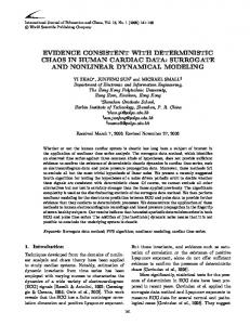
In this section we will discuss in more detail the figures of this paper. Figure 1: Projected three-dimensional plot of (a) the current J(a, b) and (b) the diffusion coefficient D(a, b) as functions of the system parameters a and b. One may notice, in part (a), close to the upper corner of the graph at a just above 2 and b just below 12 , the ‘bump’ or little ‘hill’. The existence of such a local maximum of J implies, as is not difficult to see, that what we have termed our ‘alternative ratio’, ( 12 − J)/( 21 − b), is negative in that region. As we already explained, the relation between these two effects may lose some of its mystery by realizing that both b = 0 and b = 12 are ‘symmetry points’ of the b-symmetry group of Subsection VI A, in the sense that each is a fixed point of a reflection subgroup of that symmetry group. This analogy between the two effects can also be seen simply by changing the x-coordinate and the b-parameter simultaneously over a distance 12 . Figure 2: Graphs of the diffusion coefficient D as a function of b at constant a. In parts (a)-(c) the constant values of a are respectively a = 1.125, a = 1.075 and a = 1.0375. These values are chosen so as to approach, in an approximately geometric fashion, the transition line at a = 1 between the non-chaotic and one of the two chaotic regions (the other chaotic region being located at a < −1). In part (d) these three graphs are superimposed, in a close-up containing in each case the interval of vanishing D around b = 1/3. On these graphs one may observe: (1.) As a decreases towards the limiting value 1 where the transition to non-chaotic behaviour takes place, the number of intervals with D = 0 increases rapidly whereas separate plots of J (not shown here), show that inside such intervals J has a constant, always rational value. (2.) Outside of these intervals, D(a, b) shows fractal behaviour as a function of b. (3.) Around these intervals, D(a, b) shows spikes, which usually is an indication of a critical behavior of some sort. However, from the continuity of D(a, b) throughout the chaotic region |a| > 1 [Gro] it follows that D cannot become infinite and could only become unbounded when approaching the line a = 1. This is not the case in this figure, so that the observed ‘spikes’ must be finite. This, however, leaves open the possibility that some derivative of D, in as far as it may exist, would become infinite. Elaborating a little further on the first point (1.) above, one may verify in more detail that each of these observed intervals of vanishing D is indeed determined by the intersection of the line of constant a with a respective Arnol’d tongue. This can be verified as follows: The formulas for the Arnol’d tongue boundaries presented in Section IX imply that such a tongue with J = q/p in the standard notation will extend between a = 1 and a maximum value of a given by a = 21/p so that a line of constant a will intersect those and only those Arnol’d tongues which have a p-value satisfying ap < 2. For the three graphs shown in the parts (a)-(c) of this figure this means that the maximum values of p are respectively 5, 9 and 19. With this information it is then easy to identify, in these three graphs, for each interval of vanishing D the rational value of J = q : p. For example, in part (a) one will in this way identify for the successive observed intervals with D = 0 the following values of J respectively: J = 0 : 1, 1 : 5, 1 : 4, 1 : 3, 2 : 5 and 1 : 2. A similar identification is possible for the other two graphs. In other words, the graphs of this Fig. 2 nicely illustrate the theoretical explanation given in Section IX for the existence of Arnol’d tongues in this model. Figure 3: Graphs of the current J(a, b) as a function of a, at constant b, for three different values of b. In part (a): b = 0.1, in part (b): b = 0.01 and in part (c): b = 0.001. Again, as in the case of D in the preceding figure, a highly irregular behaviour of this function emerges, which becomes wilder and wilder the closer b gets to 0. One may notice here, on comparing these three graphs, that, only roughly speaking since J has so much variation in it, each time b is scaled down by a factor 10, J also scales down but by a smaller factor; as was already necessary in order to keep all points of the curve inside the picture. This by itself is already indicative of nonlinear behaviour in b, which, however, is not so simple to describe by a single exponent since so much appears to depend on the precise value of a at which one lets b approach to 0.
18
This b-dependence of J(a, b) as b approaches to 0 appears to depend quite sensitively on the value of a. Some of this can be made more precise. For example, as can be proved from e.g. Eq. (73), for a equal to an odd integer, J = b exactly. In the general case one can say something about the range of limiting values taken by J(a, b)/b as b → 0: For general a it can be shown to be unbounded, whereas the ratio J(a, b)/(b(| log |b|)) remains bounded but has, for a general choice of a, no limit. More details will be given elsewhere [Gro]. We mention one other observation which can be made on comparing these three graphs. It is that, as b decreases towards 0, there appear more and more intervals on which J/b is negative. Figure 4: Here, the ratio J(a, b)/b is displayed as a function of 10 log b, for b ranging through eight decades from b = 1 on downwards. This is at the three different constant values of a as indicated in the figure. For each of these three values of a the current J shows a highly irregular behavior as a function of b, persisting, upon enlargements of the graph, on finer and finer scales, which is indicative of a fractal structure of J(a, b) as a function of b. Also, one observes in all three graphs that the ratio J/b is negative over rather large b-intervals. To our knowledge, this is the first finding of ‘negative currents’ in simple piecewise linear one-dimensional maps. Therefore, both effects, that of negativity of J/b and nonlinearity of J versus b, show up in these graphs, and there is no indication that eventually, from a certain small value of b on, this behaviour will disappear and a regime of linear response will be reached, i.e. where J/b would approach a constant. But the situation is a bit more complicated: There are special values of a, e.g. if a is an integer, that then, quite trivially, J(a, b) = b identically for all b. Also, this should not be confused with the ‘large field linearity’ of J(a, b) meaning that J will become asymptotically equal to b, a property which follows in an elementary way from the fact that J(a, b) − b is periodic and hence bounded so that J(a, b)/b will tend to 1. This holds quite generally under quite weak conditions for lifted circle map systems. But here at least it can be concluded that, as b increases, J(a, b) will eventually become positive and remain so. We also note that the three values of a were chosen here so as to let a approach, in a roughly geometric fashion, to the integer value a = 3, which is a value for which a plot of the ratio J/b would show no irregular behaviour at all, since this ratio then is identically equal to 1. The observation therefore is that, the closer one gets to a regular point such as a = 3, the more pronounced the singular behaviour seems to become; but that is has disappeared completely when the limiting point has been reached. Figure 5: Various close-ups of parts of the parameter plane where the phenomenon of ‘macroscopic negative response’ i.e. where J(a, b)/b < 0 takes place. In part (a), the regions where J(a, b)/b < 0 are depicted in grey, and their boundaries in black. In parts (b) and (c) further enlargements of these regions are given where only the boundaries with J(a, b) changing sign are depicted. One notices the self-similar structures which become visible; whose precise nature however is not clear yet. Figure 6: This figure is similar to Fig. 5 except that here the sign of the ‘alternative’ ratio ( 12 − J(a, b))/( 12 − b) is mapped out, instead of that of J/b. In these graphs, only the boundaries of the regions of constant sign of this ‘alternative’ ratio, i.e. the curves where J(a, b) = 12 , are depicted. Figure 7: This figure needs a longer than usual explanation because of the many details of so many different kinds it contains. We term it our ‘chart’, as it displays broadly speaking the ‘qualitative features’ of the system we have found in our preliminary survey. These features are all integer-valued which makes this two-dimensional chart possible. They are of four different types, labelled from I to IV. Those labelled I, II or III are clearly invariants of a respective, well-known invariance group, which will be indicated below. Also in the case IV a similar association seems possible. Because of the b-symmetries discussed in Subsection VI A, we have, without lack of generality, restricted our attention to the strip 0 ≤ b ≤ 21 , termed there the ‘fundamental’ strip of the parameter plane. The information displayed in this figure is in the form of a) the brackets containing three integers; b) various kinds of lines and curves, and c) the shaded areas near the two boundary lines of the graph, at b = 0 and b = 21 . − As for a): the pair of integers on top are the local values of the kneading numbers n+ 1 and n1 whereas the integer on the bottom is the number of fixed points Fix(f ) of the associated circle map f (Cf. Section III). As for b): Each curve or line is where a respective kneading number changes its value. b1) The sequence of dashed straight lines are in that way ‘indicators’ of one particular sequence of the first order kneading numbers. In the sequence of straight lines, when it has entered the non-chaotic region 0 ≤ a ≤ 1, the last one has become a boundary of an Arnol’d tongue, the one with J = 0, p = 1, q = 0. b2) The ‘zig-zagging’ sequence of curves, nearly parallel to the straight lines of b1), are ‘indicators’ in the above sense of a similar sequence kneading numbers, this time of order 2. As this sequence has entered the non-chaotic
19
region, the last one has become a boundary of the Arnol’d tongue characterized by J = 1 : 2, p = 2, q = 1. b3) Most of the other curves indicate boundaries of Arnol’d tongues. Those which are displayed prominently, in the chaotic as well as in the non-chaotic regions, are the complete sets with p-values ranging from p = 1 up to p = 5. These have been plotted using the exact equations for these boundaries of Section IX. b4) Near the line a = 1 also the boundaries of in principle all higher order (and much smaller) Arnol’d tongues are displayed. These have been plotted using the computer program implementing formula Eq. (73). b5) The dotted vertical line at a = 1 denotes the boundary between the chaotic and the non-chaotic regions, which is where the sign of the Lyapunov exponent, an invariant of Type III, changes. As for c): The shaded areas near the boundaries at b = 0 and b = 21 are where either one of the two ‘macroscopic’ responses is negative. These regions are also shown, on much larger scales, in Figs. 5 and 6. In the list below we summarize in which way, i.e. by which ones of the above listed signs (a) – (c), the information on the values of some of the invariants of the four types I-IV is displayed: (I, p and q of Section IX ; Ergodic Theory) : b3, b4. (II, Kneading numbers, Order Topology) : a, b1, b2, b3. (III, Sign of Lyapunov exponent): b5. (IV, The signs of the two current-to-bias ratios): c. XII. FURTHER PROBLEMS AND OUTLOOK
One of the features of our model of which we would like to obtain a better understanding, from a ‘physical’ or ‘probabilistic’ point of view, would be the mechanism which is responsible for the ‘ negative response’ observed in certain regions of the parameter plane. One approach would be to make a further, mathematical analysis of the explicit but subtle formula Eq. (73) for J of Section (VII) determining that sign. Another approach would be to take advantage of the connection [Kla] between the present model and certain types of ratchet models [JKH96] in which ‘negative currents’, or, in the terminology used, ‘current reversals’, also occur. The dynamical origin of the negative currents in these models is currently under discussion [Mat00,BS002]. For a recent review on ratchet models see, e.g. Ref. [Rei92]. XIII. SUMMARY
We have investigated a simple two-parameter model of chaotic dynamical transport, along lines of earlier investigations [Kla95,Kla96,KD99], but this time using as our principal tool the exact expressions for the transport properties J and D obtained recently [Gro]. These formulas are explicit and allow for a highly efficient (‘polynomial time’) computation, but analytically they are quite subtle, and the functions they represent have a fractal character. For this reason it was necessary to implement them numerically, in order to obtain at least a reasonable impression of the various properties of the model. In the course of this both numerical and analytical investigation some unexpected features of the model then came to light, as are displayed here in several figures and are amply discussed. Our most significant findings are of two kinds: 1. The ubiquitous continuous but fractal parameter dependence of every one of the ‘near-equilibrium’ transport coefficients, such as the current J = c1 and the diffusion coefficient D = c2 , throughout the chaotic part of the parameter plane, naturally with the exception of the Arnol’d tongues where they are constant anyway. Only one particular aspect of this is the ‘fractal nonlinearity’ of the current J(a, b) as a function of b, implying that, for most a-values, the limit of J/b as b → 0 does not exist. 2. A second, hitherto unexpected and thus far counter-intuitive feature of our model is the negativity of the ratio J/b in many regions of the parameter plane. This effect has two complementary versions, each relative to its respective symmetry line in the (a, b) plane. These effects occur in irregularly shaped regions which are of positive measure; and which regions close in onto the respective symmetry line, thereby showing critical behaviour. Acknowledgments The authors are indebted to J.R. Dorfman in many ways: It has each time been a privilege for J.G. to attend, during the years, the lucid and inspiring lectures by Professor Dorfman on the latest and exciting developments in Non-Equilibrium Statistical Mechanics. On one of these occasions, May 1994, he introduced a beautiful simple model, of which the one discussed in the present paper is an extension, exhibiting fascinating fractal curves, and which shortly thereafter turned out to be exactly solvable. The author wants to thank him for these lectures, for his kind interest in the present work, and for his warm hospitality during a visit, December 1996, to the University of Maryland where that solution was discussed in detail for the first time and
20
presented in a seminar. J.G. also wants to thank his colleagues and former colleagues of the Institute for Theoretical Physics in Utrecht, in particular N.G. van Kampen and Th.W. Ruijgrok, for many valuable discussions on problems of physics and mathematics. R.K. thanks J.R. Dorfman for being a wonderful teacher of physics during many years of exciting joint research on deterministic chaos and transport. Indeed, this collaboration started with R.K.’s Ph.D. thesis work on the symmetric case of the model discussed above, as initiated and supervised by Prof. Dorfman. This author furthermore wants to thank especially H. van Beijeren for his strong support of this work, as well as M.H. Ernst, P. Gaspard, G. Nicolis, G. Radons, and H. Spohn, for further support and encouragement. R.K. is currently a PKS fellow at the Max Planck Institute for Physics of Complex Systems.
AT 93 BS002
Bec93
BM W G95
CE80
Cvi02 DH87
Dor99 F LP 94
F uj82
Gan59 Gas98 Gei82
Gro Gro82
Ito81 J KH96
Kla96
Kla Kla95 KD99
Kub57 M at00
M T 88 M or90 Rei92 Sch82
vKa71
I. Antoniou and S. Tasaki, Spectral decomposition of the Ren´ yi map. J. Phys. A26, 73-94 (1993). M. Barbi and M. Salerno, Phase locking effect and current reversals in deterministic underdamped ratchets. Phys.Rev. E 62, 1988 (2002). Chr. Beck and F. Schl¨ ogl, Thermodynamics of Chaotic Systems. Volume 4 of the Cambridge Nonlinear Science Series. (Cambridge University Press, Cambridge, 1993). M. Bianucci, R. Mannella, B.J. West and P. Grigolini, From dynamics to thermodynamics: Linear response theory and statistical mechanics. Phys. Rev. E 51 , 3002-3022 (1995). P. Collet and J.-P. Eckmann, Iterated maps on the Interval as dynamical systems. Progr. in Phys. 1 (Birkh¨ auser, Boston-Basel-Stuttgart, 1980). P. Cvitanovi´c et al., Classical and Quantum Chaos. (Niels Bohr Institute, Copenhagen, 2002). E.J. Ding and P.C. Hemmer, Exact Treatment of Mode Locking for a Piecewise Linear Map. J. Stat. Phys. 48, 99-110 (1987). J.R. Dorfman, An Introduction to Chaos in Nonequilibrium Statistical Mechanics. (C.U.P., Cambridge, 1999.) L. Flatto, J.C. Lagarian and B. Poonen, The zeta function of the beta transformation. Ergod. Th. and Dynam. Sys. 14, 237-266 (1994). H. Fujisaka and S. Grossmann, Chaos-Induced Diffusion in Nonlinear Discrete Dynamics. Phys. B-Cond.Matt. 48, 261-275 (1982). F.R. Gantmacher, Applications of the Theory of Matrices. (Interscience Publ., 1959). P. Gaspard, Chaos, Scattering, and Statistical Mechanics. (Cambridge University Press, Cambridge, 1998). T. Geisel and J. Nierwetberg, Onset of diffusion and universal scaling in chaotic systems. Phys. Rev. Lett. 48, 7-10 (1982). J. Groeneveld, to be published. S. Grossmann and H. Fujisaka, Chaos-induced diffusion in nonlinear discrete dynamics. Phys. Rev. A 26, 1179-1182 (1982). R. Ito, Rotation sets are closed. Math. Proc. Cambr. Phil. Soc. 89, 107 (1981). P. Jung, J. G. Kissner and P. H¨ anggi, Regular and chaotic transport in asymmetric periodic potentials: inertia ratchets. Phys. Rev. Lett. 76, 3436-3439 (1996). R. Klages, Deterministic Diffusion in One-Dimensional Chaotic Dynamical Systems. (Wissenschaft & Technik-Verlag, Berlin, 1996). R. Klages, to be published. R. Klages and J.R. Dorfman, Simple maps with fractal diffusion coefficients. Phys. Rev. Lett. 74, 387-390 (1995). R. Klages and J.R. Dorfman, Simple deterministic dynamical systems with fractal diffusion coefficients. Phys. Rev. E 59, 5361–5383 (1999). R. Kubo, J. Phys. Soc. Jpn. 12, 570 (1957). J.L. Mat´eos Chaotic Deterministic Transport and Current Reversal in Deterministic Ratchets Phys. Rev. Lett. 84, 258-261 (2000). J. Milnor and P. Thurston On Iterated Maps of the Interval. Lecture Notes in Mathematics 1342, 465-563 (1988). M. Mori, Fredholm Determinant for piecewise linear transformations. Osaka J. Math. 27, 81-116 (1990). P. Reimann, Brownian motors: noisy transport far from equilibrium. Phys. Rep. 361 57 (2002). M. Schell, S. Fraser and R. Kapral, Diffusive dynamics in systems with translational symmetry: A one-dimensionalmap model. Phys. Rev. A 26, 504-521 (1982). N.G. van Kampen, The case against linear response theory. Acta Physica Norvegica 5, 279–284 (1971).
21
(a) J(a,b) 0.4 0.2 0
0.5 0.4 0.3 0.2 b
2 4 a
0.1
6 80
(b)
D(a,b)
2
0.5 0.4 0.3 0.2 b
1 0 2 4 a
0.1
6 80
FIG. 1. Projected three-dimensionsal plots of the current J(a, b) and the diffusion coefficient D(a, b), as functions of a and b.
22
(a)
0.002
0.00015
D(a,b)
0.0015 D(a,b)
0.0002
(c)
0.001
0.0001
0.0005
0.00005
0
0 0
0.05 0.1 0.15 0.2 0.25 0.3 0.35 0.4 0.45 0.5
0
0.05 0.1 0.15 0.2 0.25 0.3 0.35 0.4 0.45 0.5
b
(d)
0.0008
0.00035
0.0007
0.0003
0.0006
0.00025
0.0005
D(a,b)
D(a,b)
(b)
b
0.0004 0.0003
0.0002 0.00015
0.0002
0.0001
0.0001
0.00005
0 0
0.05 0.1 0.15 0.2 0.25 0.3 0.35 0.4 0.45 0.5 b
slope a=1.125 slope a=1.075 slope a=1.0375
0 0.32
0.325
0.33
0.335
0.34
0.345
b
FIG. 2. Graphs of the diffusion coefficient D as a function of b at constant a. In parts (a)-(c) a is held constant at respectively the values a = 1.125, a = 1.075 and a = 1.0375.
23
0.18
(a)
0.16 0.14
J(a,b)
0.12 0.1 0.08 0.06 0.04 0.02 1
2
3
4
5
6
7
8
5
6
7
8
5
6
7
8
a 0.03
(b)
0.02
J(a,b)
0.01 0 -0.01 -0.02 -0.03 1
2
3
4 a
0.004
(c) 0.002
J(a,b)
0 -0.002 -0.004 -0.006 -0.008 1
2
3
4 a
FIG. 3. Graphs of the current J(a, b) as a function of a at constant b. In parts (a)-(c) b is held constant at respectively the values b = 0.1, b = 0.01 b = 0.001.
24
0 -2
J(a,b)/b
-4 -6 -8 -10 slope = 3.0001 slope = 3.01 slope = 3.8
-12 -14 -16 -8
-7
-6
FIG. 4. The ratio J(a, b)/b as a function of three different values as indicated in the figure.
-5 10
-4 log b
-3
-2
-1
0
log b, with b ranging over eight decades. Herein, a is held constant at the
25
0.08 (a)
b
0.06 0.04 0.02 0
2
3
0.08
4
5 a
0.03
(b)
7
6
0.06
8
0.038
(c)
0.06 0.04
0.04 3.2
0.02 0
0.034
b
b
0.02
3
3.2
3.4
0.02
3.3
3.6
3.8
5.17 5.19 5.21 0
4
a
5
5.2
5.4
5.6
5.8
6
a
FIG. 5. Various close-ups of parts of the parameter plane where ‘macroscopic negative response’ occurs, i.e. where J(a, b)/b < 0. In part (a), regions with J(a, b)/b < 0 are coloured grey, and the boundaries thereof, which is where J changes sign, are in black. Parts (b) and (c) are further enlargements displaying now only these boundaries. Each contains an inset with a further enlargement, making the self-similar structures present in these boundary curves visible. Their precise nature is not yet clear.
26
0.5
b
0.48
0.46
0.5
0.44
4.2
4.3
4.4
0.49
0.42 2
4.1
4
a
6
8
FIG. 6. This figure is quite similar to Fig. 5 except for two differences: 1) These curves display the ‘alternative’ quantity − J(a, b) rather than the quantity J(a, b) as in the previous figure. 2) The b-scale used is different. Taking the latter into account one observes that this negativity effect starts off here earlier, i.e. around a = 2 rather than at around a = 3, and is then accordingly also larger, as compared to the case of Figure 5. 1 2
27
FIG. 7. This figure, which is our ‘chart’ of the model, displays values of invariants which are of four different types. For a detailed explanation of the figure itself see Section XI.
28