Nested sampling: an improved visual-census technique for studying ...

MARINE ECOLOGY PROGRESS SERIES Mar Ecol Prog Ser

Vol. 367: 283–293, 2008 doi: 10.3354/meps07511

Published September 11

Nested sampling: an improved visual-census technique for studying reef fish assemblages Carolina V. Minte-Vera1, Rodrigo Leão de Moura2, 3,*, Ronaldo B. Francini-Filho2, 3 1

NUPELIA - Núcleo de Pesquisas em Limnologia, Ictiologia e Aquicultura, Universidade Estadual de Maringá, Av. Colombo 5790, Bloco H-90, 87020-900 Maringá PR, Brazil 2 Programa Marinho, Conservation International Brasil, Rua das Palmeiras, 451 Centro, 45900-000 Caravelas BA, Brazil 3 Grupo de Pesquisas em Recifes de Corais e Mudanças Globais, Universidade Federal da Bahia, Rua Caetano Moura 123, 40210-340 Salvador BA, Brazil

ABSTRACT: Our aim was to devise visual sampling protocols to estimate densities in a morphologically and behaviorally diverse assemblage of reef fishes. The focus was on a design that is costeffective and produces relatively accurate and precise density estimates for the largest number of species. We evaluated the 2 most widely used shapes of sampling units (strip transects and stationary cylinders) of several dimensions on a fringing reef at Fernando de Noronha Archipelago, tropical West Atlantic. Small sampling units produced the best density estimates for small fishes, while large ones produced the best estimates for large fishes, regardless of sampling unit shape. The sampling unit with the lowest cost was the stationary cylinder. We further compared accuracy and precision of density and richness estimates from several combinations of stationary cylinders and fish size. A simple improvement in stationary censuses, i.e. a sampling unit composed of 2 nested cylinders (2 m and 4 m radii, respectively), enhanced the accuracy and precision of estimates. Counts of small fish (≤10 cm) were made in the smaller cylinder and counts of larger fish (>10 cm) were made in the larger. Such nested cylinders reduce the bias towards large and conspicuous species and allow for separate density estimates for adults and juveniles of large species. KEY WORDS: Visual census · Sampling · Reef fishes · Biodiversity · Community structure Resale or republication not permitted without written consent of the publisher

INTRODUCTION Studies focusing on biodiversity are challenged by the need to obtain precise and accurate abundance estimates for the largest possible number of species; abundance data at the assemblage level are more informative and comparable than simple species lists. There are 4 main categories of quantitative methods used to sample reef fish assemblages, i.e. video (stationary or mobile), hydroacoustic, catch-related and underwater visual census. Because of their non-invasive nature and low cost, visual-census methods are the most practical, effective and widely used protocols (Sale 1991, 1997, Samoilys 1997), although video sampling is receiving increased attention as an intermediate-cost alternative (Harvey et al. 2002, Watson et al 2005). Acoustic techniques (e.g. Cappo & Brown 1996)

are unable to differentiate most species and are of limited use for estimating diversity. Destructive sampling, while allowing for good estimates of small cryptic species (Ackerman & Bellwood 2000, Robertson & SmithVaniz 2008) is incompatible with many management objectives. Fisheries-dependent methods are limited to target species and suffer from several biases (Polunin & Roberts 1996). Since Brock’s (1954) pioneering study, several visualcensus methods have been developed, modified and improved (e.g. Thresher & Gunn 1986, Fowler 1987, Colvocoresses & Acosta 2007). Three types of visual census are most widely used: (1) plotless methods allowing for the estimation of relative abundance (e.g. Thresher & Gunn 1986), (2) strip- and line-transect methods (e.g. Fowler 1987, Bellwood & Alcala 1988) and (3) stationary-census methods (or point counts).

*Corresponding author. Email: [email protected]

© Inter-Research 2008 · www.int-res.com

284

Mar Ecol Prog Ser 367: 283–293, 2008

(2) and (3) allow density estimation (e.g. Bohnsack & Bannerot 1986). Distance-based methods (Buckland et al. 1993) are impracticable for density assessments of large numbers of small species. Visual sampling is prone to bias caused by the difficulty of seeing and enumerating individuals (Sale & Douglas 1981, DeMartini & Roberts 1982, St John et al. 1990, Sale 1997). For example, bias may be introduced by (1) a tendency to neglect small, cryptic or nocturnal species, (2) errors in species’ discrimination, counts or underwater data recording, (3) attraction or repulsion of some species by divers, (4) underwater visibility and structural complexity of habitat, and (5) differences in territorial behavior and habits of reef species (Bellwood & Alcala 1988, Sale 1997, Samoilys & Carlos 2000). An adequate sampling design (sampling unit, spatial allocation of samples and replication) contributes significantly to enhanced precision and the control of biases. While precision increases as more replicates are collected, bias cannot be corrected by replication, hence accuracy should be the main objective of sampling unit choice (Cochran 1977, Levy & Lemeshow 1991). Our aim was to investigate the most appropriate and cost-effective visual sampling unit for maximizing the number of species recorded in reef fish assemblage studies, while simultaneously providing precise and accurate species-specific density estimates. Our approach incorporated 2 widely used count protocols (strip transect and stationary cylinder) and varying sampling unit sizes, with the development of a nesting procedure for the stationary cylinder protocol. We concluded that the use of such nested samples should be considered in assemblage-level sampling designs, helping to reduce bias towards large and conspicuous species.

MATERIAL AND METHODS Study site. Sampling was conducted at a ~25 000 m2 site with a relatively homogenous topology, benthic cover and depth (7 to 12 m) located on the leeward side of Ilha do Meio, Fernando de Noronha Archipelago (03° 50’ S, 32° 25’ W), Brazil (Francini-Filho et al. 2000). During sampling (May 11 to June 11 1998), horizontal visibility ranged from 9 to 20 m, water temperature from 26 to 27.5°C, and currents from 0 to 1.8 km h–1. The reef had a slope of about 20 to 45° and was covered mostly by brown and green filamentous algae, with sparse colonies of massive corals (Montastraea, Siderastrea, Mussismillia and Porites). The reef fish assemblage. The reef fish assemblage of the Fernando de Noronha Archipelago is dominated by (1) species endemic to the eastern coast of South America and (2) wide-ranging West Atlantic species (Francini-Filho et al. 2000). A small percentage of the

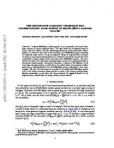
fish fauna is endemic to the Archipelago and the nearby Rocas Atoll; these endemic species are locally very abundant (Rosa & Moura 1997). The reef fishes display a wide range of behaviors, color patterns and foraging modes, and have been classified according to their ease of detection (Lincoln Smith 1988, 1989, Samoilys & Carlos 2000). Five species groups were established (Table 1). The first 2 groups (1A, 1B) comprised small species (12 cm). Only large individuals (>12 cm) of species in group 2A were recorded at the study site; group 2B was composed of species with both small juveniles and large adults in the study area, and group 2C was composed of 2 species of Halichoeres that are frequently attracted to divers. Prior to the censuses, the 2 divers counting fish spent 15 d calibrating their identification capabilities. Sampling protocols. Sampling was done by SCUBA diving between 09:00 and 17:00 h, avoiding crepuscular changeover periods. In order to assess costs, we recorded the time spent at each of the main steps of the procedures. We arbitrarily set a minimum size specification (Bellwood & Alcala 1988) of 1 cm TL for species with a maximum TL 5 cm per 4 m radius; (4) fish > 5 cm per 7.5 m radius; (5) fish ≤ 10 cm per 2 m radius; (6) fish ≤ 10 cm per 4 m radius; (7) fish >10 cm per 4 m radius; (8) fish >10 cm per 7.5 m radius (Fig. 1). The procedure was repeated 8 times by a single diver for the 10 cm size limit, and 7 times for the 5 cm size limit.

Three criteria were used to identify the most appropriate sampling unit: cost, accuracy and precision. We used higher density estimates as a proxy for accuracy (similar procedure to Colvocoresses & Acosta 2007) because underestimation is the commonest reason for reduced accuracy in visual sampling (Caughley 1977, Sale & Sharp 1983). The potential problem of a positive

4m

7.5 m

4m 4m

2m

Fig. 1. Combinations of stationary cylinder radii used in protocol 2. Shaded areas represent radii where small individuals were counted (total length TL ≤ 10 or ≤ 5 cm), outer circle Counts of small individuals delimits areas where large individuals were counted (TL >10 or > 5 cm)

Counts of large individuals

286

Mar Ecol Prog Ser 367: 283–293, 2008

relationship between fishes and the diver was minimal in this instance (see ‘Results: Protocol 1’ below). Formal estimates of accuracy would require destructive sampling either by poisons (Ackerman & Bellwood 2000) or explosives (Samoilys 1997), procedures that are now not possible in most reef environments (Robertson & Smith-Vaniz 2008). Time spent in deploying the sampling unit and performing the counts plus the number of divers required were used as cost surrogates. We quantified precision using the coefficient of variation (CV), defined as the ratio between the standard error and the estimated mean (CV (x) = SE(x) / x, Cochran 1977). Data analysis. In order to detect associations between attributes of the sampling units and species densities, we used a detrended correspondence analysis (DCA) (Hill & Gauch 1980, ter Braak 1995), computed with PC-ORD 3.15 (McCune & Mefford 1995) using the default number of segments (26) for detrending. We used a multivariate analysis of variance (MANOVA) to guide the interpretation of the DCA results, comparing the scores on the 3 first DCA axes of strip transects and stationary cylinders. Correlations between sampling unit size and density of each species were computed with Spearman rank correlation coefficients following a Bonferroni correction (Sokal & Rohlf 1995) to keep the overall probability of a Type I error equal to α = 0.05. Species accumulation curves computed in Protocol 2 were used as diversity estimators to assess the efficiency of sampling schemes (Longino & Colwell 1997). We computed the average species accumulation curve by randomly selecting 50 combinations of replicates using EstimateS 5 (available at: http://viceroy.eeb.uconn.edu/estimates).

Table 2. Cost of sampling in each shape of visual-census method Cost variable

Printed species list Number of divers Setting time (range in min) Sampling time (range in min) Total time (range in min)

Stationary cylinders

Strip transects

No 1 1–2 7–12 8–14

Yes 2 2–8 1–17 3–25

census could be obtained by each diver in a single dive. Forty-three species belonging to 25 families were observed during the study (Table 1). The first DCA axis separated species from groups 1A (small and benthic species) and 2C (medium and large species attracted to divers) from those of groups 2A and 2B (medium and large species) (Table 1, Fig. 2b). Although it is a

RESULTS Protocol 1 Stationary censuses required shorter implementation and execution times than strip transects (Table 2). Strip transects longer than 5 m required a pre-printed species list and an assistant diver for laying down the tape. Within the depth range of the present study, when the counting diver deployed the tape for transects > 5 m length, a maximum of 2 replications was achievable in a single dive with standard SCUBA. In contrast, at least 4 replications of stationary

Fig. 2. DCA ordinations of the fish assemblage (eigenvalues: axis 1 = 0.253 and axis 2 = 0.083). (a) Sampling units plot with symbol sizes proportional to sampling unit sizes. (b) Species plot showing the species groups. See Table 1 for key to species abbreviations

287

Minte-Vera et al.: Nested sampling for reef fish assemblages

small schooling fish (and the most abundant species), Thalassoma noronhanum (see Table 5) was positioned in the middle of the ordination diagram. Both strip transects and stationary cylinders overlapped in the 2-dimensional DCA plots (Fig. 2a), showing that they provided similar density estimates simultaneously for many species. Sampling unit sizes, regardless of shape, were best discriminated along the first DCA axis (Fig. 2a), with the 2 smallest sampling units significantly separated from the 3 largest (Table 3). Sampling unit area was negatively correlated with density estimates for small species (groups 1A,1B) and positively correlated with density estimates for medium and large species (group 2A, 2B; Table 4). Negative correlations of density estimates and sampling unit area were also found for species attracted to divers (group 2C). For the small species of groups 1A and 1B, the most accurate density estimates were obtained with small sampling units (transects of 2 × 1 and 5 × 1 m and stationary censuses with 1 and 2 m cylinder radii; Table 5). Densities of large species (groups 2A, 2B) were generally best estimated with larger sampling units (Table 5). In most cases, smallest sampling units produced the least precise density estimates (Table 5). Coefficients of variation generally decreased as sampling unit area increased. However, in the largest plots, precision in density estimates decreased for small species. Stegastes rocasensis and Cephalopholis fulva had least precise density estimates in the 9 m radius stationary cylinder and Ophioblennius trinitatis and Malacoctenus aff. triangulatus in the 100 × 2 m transect (Table 5). Differences between divers were stronger at the extreme cylinder sizes of 1 and 9 m radius, as shown by the significance of the interaction term in the 2-way ANOVA (Table 6, Fig. 3).

Table 3. MANOVA of the first 2 axes of the DCA and a posteriori Tukey tests (homogeneous groups at α = 0.05 linked by horizontal lines). T = strip transects of 2, 5, 10, 50 and 100 m length; S = stationary cylinders of 1, 2, 4, 7.5 and 9 m radius Strip transects Wilks λ = 0.116 Rao R = 3.625 df = 12, 34 p = 0.001 Multiple comparisons T2 T5 T10 T50 T100 Axis 1 Axis 2 Stationary cylinders Wilks λ = 0.286 Rao R = 9.073 df = 12, 180 p = 0.000 Multiple comparisons S1 S2 S4 S7.5 S9 Axis 1 Axis 2

Table 4. Spearman rank correlations between density and sampling unit size (strip transects and stationary cylinders pooled) for each species. Occurrence is the number of sampling units where the species was found (out of a total of 95). Statistically significant correlations are in bold (Bonferroni correction for Type I error: *α = 0.05/31 = 0.016 and **α = 0.01/31 = 0.00032, where 31 is the number of correlation coefficients computed) Group

Spearman Occurcorrelation rence

1A

Elacatinus cf. randalli Malacoctenus aff. triangulatus Ophioblennius trinitatis Stegastes pictus Stegastes rocasensis

0.229 –0.736** –0.331* 0.210 –0.256

7 90 74 35 79

1B

Chromis marginata Thalassoma noronhanum

0.297 –0.678**

55 95

2A

Acanthurus coeruleus Anisotremus surinamensis Carangoides spp. Chaetodon ocellatus Dasyatis americana Kyphosus sectator Melichthys niger

0.365* 0.320* 0.255 0.320* 0.186 0.309 0.553**

18 18 6 15 4 6 34

2B

Abudefduf saxatilis Acanthurus chirurgus Cephalopholis fulva Haemulon chrysargyreum Holocentrus ascensionis Lutjanus jocu Mulloides martinicus Myripristis jacobus Pempheris schomburgki Pomacanthus paru Pseudupeneus maculatus Sparisoma frondosum Sparisoma radians Sparisoma axillare Sparisoma amplum

0.213 0.392 0.141 0.335* 0.473** 0.350* 0.297 0.227 0.265 0.257 0.053 0.377* –0.290 0.492** 0.256

33 42 64 9 29 11 9 13 3 5 50 57 73 29 9

2C

Halichoeres dimidiatus Halichoeres radiatus

–0.037 –0.687**

57 86

Protocol 2 Results from the first protocol indicated that fish size is one of the key factors to be taken into account in choosing the best sampling unit. In general, density of small species was estimated with higher accuracy with smaller sampling units, while the density of large species was estimated with higher accuracy with larger sampling units. A second experiment using only stationary cylinders was designed to define a more objective size limit between small and large fish, and also to determine the best sampling unit for these categories. For small fish, the size limits of 5 and 10 cm TL produced similar density estimates in the 2 radii of stationary cylinders (2 and 4 m, Fig. 4). However, these estimates were more precise for size limits of 10 cm TL. For larger fish, the same trend in precision was observed

Species

288

Mar Ecol Prog Ser 367: 283–293, 2008

Table 5. Density estimates (x, ind. m–2) and coefficient of variation (CV) for the 15 most abundant species. See Table 1 for full generic names of fish

Radius (Area) Species Group 1A M. aff. triangulatus O. trinitatis S. pictus S. rocasensis

1m (3.1 m2) x CV

2m (12.6 m2) x CV

Stationary cylinders 4m (50.2 m2) x CV

7.5 m (176.6 m2) x CV

9m (254.3 m2) x CV

2.28 0.20 0.02 0.28

18.5 40.1 100 41.6

0.99 0.30 0.02 0.34

15.2 12.3 53.7 16.6

0.28 0.10 0.01 0.10

17.8 23.9 57.5 19.4

0.09 0.03 < 0.01< 0.05

12.1 22.7 40.7 17.4

0.05 0.03 < 0.01< 0.03

20.4 22.7 39.4 29.3

0.16 24.800

75.3 15.5

1.250 14.51

31.4 12.5

1.05 11.75

35.6 13.7

0.99 4.90

31.0 15.2

0.39 4.79

30.6 16.3

Group 2A M. niger

0.02

100

0.01

68.3

< 0.01

72.4

0.01

20.1

0.03

29.8

Group 2B A. chirurgus A. saxatilis C. fulva P. maculatus S. frondosum S. radians

0.26 0.10 0.12 0.14 0.02 0.40

100 63.5 41.3 35.9 100 24.8

0.12 0.04 0.08 0.08 0.05 0.47

45.9 62.5 32.9 32.7 35.4 19.6

0.14 0.02 0.04 0.02 0.03 0.13

54.0 35.4 17.6 51.3 31.1 26.9

0.06 0.02 0.04 0.01 0.03 0.06

34.2 23.9 6.5 21.9 10.0 24.3

0.09 < 0.01< 0.04 0.01 0.02 0.05

37.1 47.9 41.8 32.6 15.0 23.3

Group 2C H. radiatus H. dimidiatus

0.46 0.12

14.2 33.3

0.22 0.05

20.3 28.7

0.06 0.03

13.3 22.9

0.03 < 0.01
1.5 × larger than the interquantile range. (b) Twoway interaction (diver × radius) plot for log transformed means of total number of individuals counted per diver, F (4, 65) = 2.53; p < 0.05

Fig. 4. Average density (ind. m–2) and corresponding coefficient of variation (CV) for fish with total length (TL) ≤5 cm and TL ≤10 cm in stationary cylinders of 2 (a,b) and 4 m (c,d) radius. Solid line represents the 1:1 relationship. See Table 1 for species abbreviations

290

Mar Ecol Prog Ser 367: 283–293, 2008

Fig. 5. Average density (ind. m–2) and corresponding coefficient of variation (CV) for fish with total length (TL) > 5 cm and TL >10 cm in stationary cylinders of 4 (a,b) and 7.5 m (c,d) radius. Solid line represents the 1:1 relationship. See Table 1 for species abbreviations

Fig. 6. (a) Average density (ind. m–2) and (b) corresponding coefficient of variation (CV) for small fish (total length TL ≤10 cm) in stationary cylinders of 2 and 4 m radius. Solid line represents the 1:1 relationship. See Table 1 for species abbreviations

Fig. 7. (a) Average density (ind. m–2) and (b) corresponding coefficient of variation (CV) of fish ≤10 cm TL in stationary cylinders of 4 and 7.5 m radius. Solid line represents the 1:1 relationship. See Table 1 for species abbreviations

tionary cylinder), and (1) fish size and (2) behaviour. The correspondences lead us to evaluate a second protocol, consisting of 2 differently sized nested stationary cylinders within each of which fish of different sizes were counted (small fish in the smaller cylinder, larger fish in the larger cylinder).

DCA is an approximation of the bell-shaped response of species abundance to an environmental gradient (see ter Braak 1995). For evaluating sampling design, the species location on the ordination diagram can be seen as the optimum response to a corresponding sampling unit (i.e. highest density estimate).


291

Fig. 8. Average species accumulation curve for randomly selected sequences of combined sampling units used to sample small fish (stationary cylinders with radius 2 or 4 m) and medium or large fish (stationary cylinders with radius 4 and 7.5 m). Boxes indicate the cumulative number of species for a cumulative area of 500 m2 obtained from a combination of large and small stationary cylinders

Higher density estimates were more related to fish size and sampling unit size than to fish behavior and sampling unit shape (Fig. 2). Scores of most small, benthic, and territorial species (group 1A) corresponded to those of small-sized sampling units, while those of medium to large species (groups 2A and 2B) corresponded to large sampling units, regardless of shape. Transects and stationary censuses provided similar density and diversity estimates in the species-poor assemblages we studied; this similarity between census procedures has also been demonstrated in speciesrich Indo-Pacific reef fish assemblages (Samoilys & Carlos 2000). Our multiple density estimates were less influenced by fish behavior (e.g. solitary versus schooling) and habitat use (benthic versus pelagic) than fish length. We suggest that variation in behavior and habitat use would not compromise the use of higher density estimates as a proxy for accuracy when multiple species are sampled simultaneously. Although 2 species of Halichoeres were found to be attracted to divers, they were not overly abundant in the assemblage and do not compromise our main conclusions. The least abundant species, such as Pempheris schomburgki and Cryptotomus roseus, were scattered at the margins of the DCA ordination diagram, as is usual in such analyses (e.g. ter Braak 1995). Widely distributed and abundant species were concentrated in the middle of the plot (e.g. Thalassoma noronhanum, group 1B). Chromis marginata, another small species that aggregates in the water column (group 1B), was not as abundant as T. noronhanum and occurred in

denser aggregations, and had a more peripheral position in the ordination diagram (Fig. 2). Indeed, dense schools of small fish such as C. marginata may be as readily detected as larger and more conspicuous fish, and small schooling fish density is best estimated with larger sampling units. Transects produced estimates similar to stationary cylinders, but were less cost-effective. The cylindrical shape of the stationary census guarantees a smaller border effect (Krebs 1999), implying that fewer decisions need to be made about whether a fish is within or outside the sampling unit, although any error in the determination of boundaries will be squared in a cylindrical sampling unit (Samoilys & Carlos 2000). For these reasons, only cylindrical stationary sampling was considered in the second protocol. The second protocol targeted the relationship between fish size and sampling unit size, supporting the correspondence between these variables and identifying combinations of radii that produced the best density and richness estimates. It also helped outline a more objective size limit between ‘small’ and ‘large’ fish. Size limits of 5 and 10 cm TL produced similar density estimates in the 2 radii (2 and 4 m, Fig. 4). Since accuracy was similar for both size limits, the 10 cm size threshold was preferred because it produced the most precise estimates. For larger fish, the same trend in precision was observed (Fig. 5), leading us to conclude that the best fish size threshold to discriminate sampling unit size is 10 cm TL. In addition to errors in species discrimination, which are controlled through taxonomic calibration, variation

Mar Ecol Prog Ser 367: 283–293, 2008

292

among observers can be affected by the sampling unit size. Stationary censuses with extreme sizes (1 and 9 m radii) resulted in larger variability between observers than those with radii of 2, 4 and 7.5 m. In the smallest cylinders, the degree of aggregation and diver interference may account for the large between-diver variability. In the largest cylinders, the diver has to make more decisions on whether or not to count an individual fish near the border, and variations in water visibility may amplify bias. Whatever the factor interaction causing these largest variations may be, it is clear that ‘intermediate’-sized plots produce less variable estimates (see also Bohnsack & Bannerot 1986, Samoilys & Carlos 2000). Although the best combination of size limit and cylinder radius might vary with local circumstances and questions being explored, we suggest that nested stationary cylinders be considered in pilot studies to determine optimal sampling units for reef fish assemblages. The use of nested cylinders also allows separate estimation of adult and juvenile densities for large species, and may be easily adapted to record other size categories. Nested stationary cylinders with 2 and 4 m radii for counting small (TL ≤ 10 cm) and large (TL > 10 cm) individuals, respectively, produced the most accurate density estimates for large and small fish, and also had the highest rate of increase in the species accumulation curve (Fig. 8). Nesting two stationary cylinders of different size and counting different size categories of fish within the 2 radiii is a simple improvement that provides the best compromise among cost, accuracy and precision of density for the largest possible number of species.

Acknowledgements. We thank E. Silva, L. Kaufman, G. Dutra, R. Castro and anonymous referees for valuable comments and discussions, J. Choat for editorial assistance, M. Rodrigues, L. Mendes, F. Pereira and M. Villela for field assistance, Parque Nacional Marinho de Fernando de Noronha/IBAMA for logistical support and research permits, Centro Golfinho Rotador (through J. Silva Jr.) for logistical support; FAPESP (grants to R.L.M and R.B.F.F.) and FINEP/PRONEX (grant to N. Menezes) for funding. This is contribution number 6 of the Brazil Node of the Marine Managed Areas Science Program at Conservation International.

LITERATURE CITED

➤ Ackerman ➤

JL, Bellwood DR (2000) Reef fish assemblages: a re-evaluation using enclosed rotenone stations. Mar Ecol Prog Ser 206:227–237 Bellwood DR, Alcala AC (1988) The effect of a minimum length specification on visual estimates of density and biomass of coral reef fish. Coral Reefs 7:23–27 Bohnsack JA, Bannerot SP (1986) A stationary visual census technique for quantitatively assessing community structure of coral reef fishes. NOAA Tech Rep 41:1–15

Brock VF (1954) A preliminary report on a method of estimating reef fish populations. J Wildl Manage 18:299–308 Buckland ST, Anderson DR, Burnham KP, Laake JL (1993) Distance sampling. Estimating abundance of biological populations. Chapman & Hall, London Cappo M, Brown IA (1996) Evaluation of sampling methods for reef fish populations of commercial and recreational interest. CRC Reef Research Centre Technical Report No. 6. CRC Reef Research Centre, Townsville ➤ Caughley G (1977) Sampling in aerial survey. J Wildl Manage 41:605–615 Cochran WG (1977) Sampling techniques. Wiley, New York ➤ Colvocoresses J, Acosta A (2007) A large-scale field comparison of strip transect and stationary point count methods for conducting length-based underwater visual surveys of reef fish populations. Fish Res 85:130–141 ➤ De Girolamo M, Mazzoldi C (2001) The application of visual census on Mediterranean rocky habitats. Mar Environ Res 51:1–16 ➤ DeMartini E, Roberts D (1982) An empirical test of bias in the rapid visual technique for species-time censuses of reef fish assemblages. Mar Biol 70:129–134 ➤ Fowler AJ (1987) The development of sampling strategies for population studies of coral reef fishes. A case study. Coral Reefs 6:49–58 Francini-Filho RB, Moura RL, Sazima I (2000) Cleaning by the wrasse Thalassoma noronhanum, with two records of predation by its grouper client Cephalopholis fulva. J Fish Biol 56:802–809 ➤ Harvey E, Fletcher D, Shortis M (2002) Estimation of reef fish length by divers and by stereo-video — a first comparison of the accuracy and precision in the field on living fish under operational conditions. Fish Res 57:255–265 ➤ Hill MO, Gauch HG (1980) Detrended correspondence analysis: an improved ordination technique. Vegetatio 42:47–58 Krebs CJ (1999) Ecological methodology, 2nd edn. AddisonWelsey Educational Publishers, Menlo Park, CA Levy PS, Lemeshow S (1991) Sampling of populations: methods and applications. John Wiley & Son, New York ➤ Lincoln Smith MP (1988) Effects of observer swimming speed on sample counts of temperate rocky reef fish assemblages. Mar Ecol Prog Ser 43:223–231 ➤ Lincoln Smith MP (1989) Improving multispecies rocky reefs fish censuses by counting different groups of species using different procedures. Environ Biol Fishes 26:29–37 ➤ Longino JT, Colwell RK (1997) Biodiversity assessment using structured inventory: capturing the ant fauna of a tropical rain forest. Ecol Appl 7:1263–1277 ➤ McCormick MI, Choat JH (1987) Estimating total abundance of a large temperate-reef fish using visual strip-transects. Mar Biol 96:469–478 McCune B, Mefford MJ (1995) PC-ORD. Multivariate analysis of ecological data. Version 3.15. MjM Software Design, Gleneden Beach, OR Polunin NVC, Roberts CM (1996) Reef fisheries. Chapman & Hall, London ➤ Robertson DR, Smith-Vaniz WF (2008) Rotenone: an essential but demonized tool for assessing marine fish diversity. Bioscience 58:165–170 Rosa RS, Moura RL (1997) Visual assessment of reef fish community structure in the Atol das Rocas Biological Reserve, off Northeastern Brazil. Proc 8th Int Coral Reef Symp 1:983–986 Sale PF (1991) Reef fish communities: open non-equilibrial systems. In: Sale PF (ed) The ecology of fishes on coral reefs. Academic Press, San Diego, CA, p 564–598 Sale PF (1997) Visual census of fishes: How well do we see


what is there? Proc 8th Int Coral Reef Symp 2:1435–1449

➤ Sale PF, Douglas WA (1981) Precision and accuracy of visual ➤

➤

census technique for fishes assemblages on coral patch reefs. Environ Biol Fishes 6:333–339 Sale PF, Sharp BJ (1983) Correction for bias in visual transect censuses of coral reef fishes. Coral Reefs 2:37–42 Samoilys MA (1997) Manual for assessing fish stocks on Pacific coral reefs. Department of Primary Industries, Queensland. Training Series QE 97009, Brisbane Samoilys MA, Carlos G (2000) Determining methods of underwater visual census for estimating the abundance of coral reef fishes. Environ Biol Fishes 57:289–304 Sokal RR, Rohlf FJ (1995) Biometry, 3rd edn. WH Freeman, New York Editorial responsibility: Howard Choat, Townsville, Queensland, Australia

293

➤ St John J, Russ GR, Gladstone W (1990) Accuracy and bias of

➤ ➤

visual estimates of numbers, size structure and biomass of a coral reef fish. Mar Ecol Prog Ser 64:253–262 ter Braak CJK (1995) Ordination. In: Jongman RHG, ter Braak CJF, Van Tongeren OFR (eds) Data analysis in community and landscape ecology. Cambridge University Press, Cambridge Thresher RE, Gunn JS (1986) Comparative analysis of visual census techniques for highly mobile reef associated piscivores (Carangidae). Environ Biol Fishes 17:93–116 Watson DL, Harvey ES, Anderson MJ, Kendrick GA (2005) A comparison of temperate reef fish assemblages recorded by three underwater stereo-video techniques. Mar Biol 148:415–425 Submitted: September 12, 2006; Accepted: April 7, 2008 Proofs received from author(s): August 13, 2008