[4] Yosee Feldman and Ehud Shapiro. Spatial machines: a more realistic approach to parallel computation. Communications of ACM, 35(10):60{73, 1992.
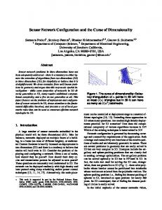
NetQTM: Node Configuration In Network Setup By Quantum Turing Machine Mehdi Bahrami1, Peyman Arebi2, Mohammad Bahrami1 1
Department of Computer Engineering, Islamic Azad University, Booshehr Branch, Iran 2 The Holy Prophet Higher Education Complex, Booshehr, Iran
Abstract - The quantum Turing machine (QTM) has been introduced by Deutsch as an abstract model of quantum computation. In this paper we try to introduction the new transition function of a QTM can be used for any node configuration in the network. In this paper we introduce the fundamentals of NetQTM like a well-observed lemma and a completion lemma. The introduction of such an abstract machine allowing classical and quantum computations is motivated by the emergence of models of quantum computation like the one-way model. Furthermore, this model allows a formal and rigorous treatment of problems requiring classical interactions, like the halting[8] of QTM. Finally, it opens new perspectives for the construction of a universal QTM. Keywords: QTM, NetQTM, Quantom Turing Machin, Node Configuration 1.
Introduction
A Turing machine (TM)[1] is a basic abstract symbolmanipulating machine which can simulate any computer that could possibly be constructed. A Turing machine that is able to simulate any other Turing machine is called a Universal Turing machine (UTM, or simply a universal machine) [17, 18 and 19]. Studying abstract properties of TM and UTM yields many insights into computer science and complexity theory [2, 3, and 4]. Turing and others proposed mathematical computing models allow the study of algorithms independently of any particular computer hardware. This abstraction is invaluable [16]. 2.
Informal Description
A Turing machine consists of: - A tape - A head - A table - A state register
A tape is divided into cells, one next to the other. Each cell contains a symbol from some finite alphabet. The alphabet contains a special blank symbol (here written as 'B') and one or more other symbols [5,6]. The tape is assumed to be arbitrarily extendable to the left and to the right. Cells that have not been written to before are assumed to be filled with the blank symbol. In some models: - The tape has a left end marked with a special symbol - The tape extends or is indefinitely extensible to the right A head can read and write symbols on the tape and move the tape left and right one (and only one) cell at a time. In some models the head moves and the tape is stationary. A table (transition function) [9] of instructions (usually 5tuples but sometimes 4-tuples) for: - The state the machine is currently in and - The symbol it is reading on the tape tells the machine what to do [7]. In some models, if there is no entry in the table for the current combination of symbol and state then the machine will halt. Other models require all entries to be filled. In case of the 5-tuple models: (i) Either erase or write a symbol, and then (ii) Move the head ('L' for one step left or 'R' for one step right), and then (iii) Assume the same or a new state as prescribed. In the case of 4-tuple models: (ia) erase or to write a symbol or (ib) move the head left or right, and then (ii) Assume the same or a new state as prescribed, but not both actions (ia) and (ib) in the same instruction. A state register stores the state of the Turing table. The number of different states is always finite and there is one special start state with which the state register is initialized. 3. A
Formal Description (one-tape)
Turing machine where - Q is a finite set of states
is
a
7-tuple
- > is a finite set of the tape alphabet/symbols is the blank symbol - @, a subset of > not including b, is the set of input symbols is the transition function, where L is left shift and R is right shift. is the initial state is the set of final or accepting states Example – Copy String
The computation itself, i.e. the TM’s time evolution, is determined by a so-called transition function δ: depending on the current state of the control q ∈ Q and the symbol σ∈Σ which is on the tape cell where the head is pointing to, the TM turns into some new internal state q'∈Q, writes some symbol σ'∈Σ onto this tape cell, and then either turns left (L) or right (R). Thus, the transition function δ is a map δ: Q × Σ → Q × Σ × {L,R}. As an example, we consider a TM with alphabet Σ = {0, 1,#}, internal states Q = {q0, q1, qf} and transition function δ , given by
In 1985, Deutsch [10] proposed the first model of a quantum Turing machine (QTM), elaborating on an even earlier idea by Feynman [11]. Bernstein and Vazirani [12] worked out the theory in more detail and proved that there exists an efficient universal QTM (it will be discussed in Section 2.2 in what sense). A more compact presentation of these results can be found in the book by Gruska [14]. Ozawa and Nishimura [13] gave necessary and sufficient conditions that a QTM ’ s transition function results in unitary time evolution. Benioff [15] has worked out a slightly different definition which is based on a local Hamiltonian instead of local transition amplitude [18]. The definition of QTMs that we use in this paper will be completely equivalent to that by Bernstein and Vazirani. Yet, we will use some different kind of notation which makes it easier (or at least clearer) to derive ana-lytic estimates like “ how much does the state of the control change at most, if the input changes by some amount?” Also, we use the word QTM not only for the model itself, but also for the partial function which it generates.
We can define δ at these arguments in an arbitrary way. We imagine that this TM is started with some input bit string s, which is written onto the tape segment [0, L(s)-1]. The head initially points to cell number zero. The computation of the TM will then invert the string and halt. As an example, in Figure 2.1, we have depicted the first steps of the TM’s time evolution on input s = 10. A QTM is now defined analogously as a TM, but with the important difference that the transition function is replaced by transition amplitude. That is, instead of having a single classical successor state for every internal state and symbol on the tape, a QTM can evolve into a superposition of different classical successor states.
4.
NetQTM
To understand the notion of a quantum Turing machine (QTM), we first explain how a classical Turing machine (TM) is defined. We can think of a classical TM as consisting of three different parts: a control C, a head H, and a tape T. The tape consists of cells that are indexed by the integers, and carry some symbol from a finite alphabet Σ. In the simplest case, the alphabet consists of a zero, a one, and special blank symbol #. At the beginning of the computation, all the cells are blank, i.e. carry the special symbol #, except for those cells that contain the input bit string. The head points [24] can connect to one of the cells. It is connected to the control, which in every step of the computation is in one “internal state” q out of a finite set Q. At the beginning of the computation, it is in the initial state q0 ∈ Q, while the end of the computation (i.e. the halting of the TM) is attained if the control is in the so-called final state qf ∈ Q.
Figure 1: Time evolution of a Turing machine
For example, we may have a QTM that, if the control’s internal state is q0 ∈ Q and the tape symbol is a 0, may turn into internal state q1 and write a one and turn right, as well as writing a zero and turning left, both at the same time in superposition, say with complex amplitudes
Figure 2: One step of time evolution of a quantum Turing machine
For our purpose, it is useful to consider a special class of QTMs with the property that their tape T consists of two different tracks an input track I and an output track O. [21 ,22] This can be achieved by having an alphabet which is a Cartesian product of two alphabets, in our case Σ = {0, 1,#} × {0, 1,#} [23]. Then, the tape Hilbert space HT can be written as thus:
A symbolic picture of this behavior is depicted in Figure 2. This can be written as 5.
Formally, the transition amplitude δ is thus a mapping from Q × Σ to the complex functions on Q×Σ× {L, R}. If the QTM as a whole is described by a Hilbert space HQTM, then we can linearly extend δ to define some global time evolution on HQTM. We have to take care of two things: • According to the postulates of quantum mechanics, we have to construct δ in such a way that the resulting global time evolution on HQTM is unitary. • The complex amplitudes which are assigned to the successor states have to be efficiently computable, which has the physical interpretation that we should be able to efficiently prepare hardware (e.g. some quantum gate) which realizes the transitions specified by δ. Moreover, this requirement also guarantees that every QTM has a finite classical description, that there is a universal QTM (see discussion below), and that we cannot “hide” information (like the answer to infinitely many instances of the halting problem) in the transition amplitudes. Consequently, Bernstein and Vazirani [4] define a quantum Turing machine M as a triplet (Σ,Q, δ), where Σ is a finite alphabet with an identified blank symbol #, Q is a finite set of states with an identified initial state q0 and final state qf 6= q0, and is the so-called the quantum transition function, determining the QTM’s time evolution in a way which is explained below. Here, the symbol denotes the set of complex numbers that are efficiently computable. In more detail, if and only if there is a deterministic algorithm that computes the real and imaginary parts of α to within 2-n in time polynomial in n. Every QTM evolves in discrete, integer time steps, where at every step, only a finite number of tape cells is non-blank. For every QTM, there is a corresponding Hilbert space where HC = CQ is a finite-dimensional Hilbert space spanned by the (or-thonormal) control states q ∈ Q, while are separable Hilbert spaces describing the contents of the tape and the position of the head. In this definition, the symbol T denotes the set of classical tape configurations [20] with finitely many non-blank symbols, i.e.
Conclusion
In this paper, we have formally defined Network Configuration Quantum Turing Machine, based on QTM, and have given rigorous mathematical proofs of its basic properties. In particular, we have shown that the quantum complexity notions can use for every node configuration on the network and recognize by other node or transfer data by transfer function on the QTM properties.
6. References Paul Benio_. Models of quantum turing machines. Fortschritte der Physik, 46:423, 1998. [2] Gilles Brassard. Quantum computing: the end of classical cryptography? SIGACT News, 25(4):15{21, 1994. [3] Marco Carpentieri. On the simulation of quantum turing machines. The-ory of Computer Science, 304(13):103{128, 2003. [4] Yosee Feldman and Ehud Shapiro. Spatial machines: a more realistic approach to parallel computation. Communications of ACM, 35(10):60{73, 1992. [5] Joel David Hamkins. In_nite time Turing machines. Minds and Machines,12(4):521{539, 2002. [6] Toby Ord. Hypercomputation: computing more than the Turing machine. CoRR, Department of Computer Science, University of Melbourne, 2002. [7] Alon Orlitsky, Narayana P. Santhanam, and Junan Zhang. Always good Turing: Asymptotically optimal probability estimation. focs '03: Pro-ceedings of the 44th annual ieee symposium on foundations of computer science, vol 302, no 5644. pages 427{431, 2003. [8] Alan Turing. Halting problem of one binary horn clause is undecidable. pages Ser. 2, Vol. 42, 1937. [9] M. Ozawa and H. Nishimura, “ Local Transition Functions of Quantum Turing Machines ” , Theoret. Informatics and Appl. 34 379-402, 2000. [10] D. Deutsch, “ Quantum theory, the Church-Turing principle and the universal quantum computer”, Proc. R. Soc. Lond. A400,1985. [11] R. Feynman, “Simulating physics with computers”, International Jour-nal of Theoretical Physics 21 467-488, 1982. [12] E. Bernstein, U. Vazirani, “ Quantum Complexity Theory”, SIAM Jour-nal on Computing 26 1411-1473, 1997. [1]
[13]
[14] [15] [16] [17]
[18]
[19]
A. A. Brudno, “ Entropy and the complexity of the trajectories of a dynamical system ”, Trans. Moscow Math. Soc. 2 127-151, 1983. J. Gruska, Quantum Computing, McGraw–Hill, London (1999) P. Benioff, “Models of Quantum Turing Machines”, Fortsch. Phys. 46 423-442, 1998. A. S. Holevo, “Statistical Structure of Quantum Theory”, Springer Lecture Notes 67, 2001. R. Jozsa, M. Horodecki, P. Horodecki and R. Horodecki, “ Universal Quantum Information Compression ” , Phys. Rev. Lett. 81 1714-1717, 1998. A. Kaltchenko, E. H. Yang, “Universal compression of ergodic quantum sources”, Quantum Information and Computation 3, No. 4 359-375, 2003. G. Keller, Wahrscheinlichkeitstheorie, “Lecture Notes, Universit¨at Erlangen-N¨urnberg , 2003.
[20]
[21]
[22] [23] [24]
J. Kieffer, “ A unified approach to weak universal source coding”, IEEE Trans. Inform. Theory 24 No. 6 674-682, 1978. A. N. Kolmogorov, “ Three Approaches to the Quantitative Definition on Information”, Problems of Information Transmission 1 4-7, 1965. K. Kraus, “States, Effects, and Operations: Fundamental Notions of Quantum Theory”, Springer Verlag, 1983. M. Li and P. Vitanyi, An Introduction to Kolmogorov Complexity and Its Applications, Springer Verlag, 1997. Mehdi Bahrami, Peyman arebi, "A Binomial Heap Algorithm for Self-Recognition in Exclusive Management on Autonomic Grid Networks", 2nd Int Conference on Computational Intelligence, Communication Systems and Networks - 14-N Parallel and Distributed Architectures and Systems, pp. 326 329 , 2010.