These units monitor network traffic, performing local analysis of that traffic and reporting attacks to a central management console. The network-based intrusion ...
IJCA Special Issue on “Network Security and Cryptography” NSC, 2011
Network Anomaly Detection using Unsupervised Model Prasanta Gogoi
Bhogeswar Borah
Dhruba K Bhattacharyya
Dept. of Computer Sc.& Engg. Tezpur University, India
Dept. of Computer Sc.& Engg. Tezpur University, India
Dept. of Computer Sc.& Engg Tezpur University, India
ABSTRACT Most existing network intrusion detection systems use signaturebased methods which depend on labeled training data. This training data is usually expensive to produce due to cost of laboratory set up, experienced or knowledge person and non availability of ready software tool. Above all, these methods have difficulty in detecting new or unknown types of attacks. Using unsupervised anomaly detection techniques, however, the system is capable of detecting previously unknown attacks without labeled training data. In this paper, we have discussed anomaly based network intrusion detection and proposed two unsupervised clustering algorithms for anomaly detection. The algorithms are evaluated with our generated real life intrusion dataset. The dataset is created with extracted features of captured network packet as well as flow traffic. The algorithm is also tested and validated with standard KDD Cup 1999 dataset and NSL-KDD dataset. The results are compared with results of similar algorithms and have been found excellent.
General Terms Intrusion Detection, Unsupervised Classification, Detection Rate
Keywords Intrusion, Unsupervised, Supervised, Anomaly, Clustering, TPR, FPR
1. INTRODUCTION With the evolutionary expansion of network-based computer services, the security measure against computer and network intrusions is a crucial issue in a computing environment. The intrusions or attacks to the computer or network system are the activity or attempt to destabilize it by compromising the security in confidentiality, availability or integrity of the system. As defined in [1], intrusion detection system (IDS) is the process of monitoring the events occurring in a computer system or network and analyzing them for signs of intrusions. A networkbased IDS (NIDS) often consists of a set of single-purpose sensors or host computers placed at various points in a network. These units monitor network traffic, performing local analysis of that traffic and reporting attacks to a central management console. The network-based intrusion detection are broadly studied in two approaches [2] : rule based and anomaly-based. Rule based (also called misuse-based) detection searches for specific pattern (or intrusion signature of rules) in the data effectively detecting previously known intrusions. Snort [3] is a widely used rule-based NIDS and it can detect intrusions of previously known intrusion signature patterns. Rule-based approach usually, do not generate large number of false alarms of detection since it is based on rules of known intrusions but it fails to detect new types of intrusions as their signatures are not known. Anomaly detection consists of analyzing and reporting
unusual behavioral patterns in computing systems. Anomaly based detection approach, typically, builds a model of normal behavior from the observed data and distinguishes any significant deviations or exceptions from this model. Anomaly based detection implicitly assumes that any deviation from normal behavior is anomalous. Anomaly detection approach has the ability to examine new or unknown intrusions. Based on learning method, anomaly detection can be of two different categories [4]: supervised and unsupervised. In supervised anomaly detection, normal behavior model of systems or networks are established by training with labeled or purely normal dataset. These normal behavior models are used to classify new network connections and gives alert if a connection is classified to be maligned or abnormal behavior. ADAM [5] is a supervised anomaly-based as well as misuse-based NIDS. However, in practice, to train a supervised anomaly-based method, labeled or purely normal data are not easily available. Since it is time consuming to acquire and error prone in manual classifying the label as benign or malign. Whereas, unsupervised anomaly detection approaches work without any training data or these models may be trained on unlabeled or unclassified data and it attempts to find intrusions lurked inside the data. A number of IDSs employ unsupervised anomaly-based approaches [6,7,8]. The most prevalent advantage of anomaly detection approach is the detection of unknown intrusions without any previous knowledge of intrusions. However, it fails to detect or false detection rate tends to be higher if behavior of some of intrusions are not significantly different from considered normal behavior model. In network-based intrusion detection, usually, threat arises from new or previously not known intrusions. The possible detection approach of novel intrusions is anomaly-based detection approach instead of rule based approach. In anomaly-based supervised detection approach, obtaining labeled or purely normal data is a critical issue. Unsupervised anomaly-based detection can address this issue of novel intrusion detection without prior knowledge of intrusions or purely normal data. In literature [9,8,10,11] clustering is established as a useful method for anomaly-based unsupervised detection of intrusions. From classical definition of data mining, clustering is a method of grouping of objects based on similarity of the objects. The similarity within a cluster is more and dissimilarity among clusters are distinct. Clustering itself is a kind of unsupervised study method [12]. This method can be carried on unlabeled data, it divides the similar data to the same class and divides the dissimilar data to different classes. Unsupervised anomaly-based detection often tries to cluster test dataset into groups of similar instances which may be either intrusion or normal data. Although, using of clustering method in unsupervised anomaly based detection for intrusion, generate many clusters, labeling clusters is still a difficult issue faced by this approach. In order
19
IJCA Special Issue on “Network Security and Cryptography” NSC, 2011 to label clusters, unsupervised anomaly-based detection approach model normal behavior by using two assumptions [4] (i) the number of normal instances vastly outnumber the number of anomalies and (ii) anomalies themselves are qualitatively different from the normal instances. If these assumptions hold, intrusions can be detected based on cluster sizes. Larger clusters correspond to normal data, and smaller clusters correspond to intrusions. But this method is likely to produce higher false detection rate as the assumptions are not always true in practice. For example, in denial of service category of intrusions a large number of very similar instances are generated that may form larger clusters than normal behavior cluster. On the other hand in remote to local (r2l) and user to root (u2r) categories of intrusion, legitimate and illegitimate users are difficult to distinguish. These intrusions may include normal behavior model. Consequently, these can rise the false detection rate.
1.1 Motivation Our motivation of this work is to build an efficient and effective clustering based algorithm for detection of novel intrusions by allowing training with unlabeled data. Its efficiency and effectiveness will be the higher detection rate and the lower false detection comparing to the existing approaches of unsupervised intrusion detection.
1.2 Contribution In this work we developed two clustering based algorithms called k-point-1 and k-point-2 for unsupervised anomaly based intrusion detection. We evaluate the approaches with our generated intrusion dataset and well-known benchmark intrusion dataset KDD Cup 1999 [13]. Also, we evaluate the approach with NSL-KDD dataset [14] which is a filtered dataset from KDD Cup 1999 dataset. We compare results of our approach with similar existing approaches.
1.3 Organization The remainder of this paper is organized as follows. Section 2, summarizes the related work on k-point-1 and k-point-2 algorithms. In section 3, we describe the proposed clustering algorithms for unsupervised and supervised anomaly detection. Section 4 reports the evaluation results of the proposed algorithms. Finally, section 5 concludes with future direction of research.
2. Related work Applying clustering in unsupervised anomaly-based detection of network intrusion is a wide research area that has drawn interest in the academic community. Portnoy, et. al. [4] presents a clustering based unsupervised anomaly detection algorithm in order to detect new intrusions. The training dataset containing unlabeled data is clustered using a modified incremental kmeans algorithm. Each cluster is labeled as normal or intrusive based on the number of instances in the cluster. Some percentage of the clusters containing the largest number of instances are labeled as normal and the rest of the clusters are labeled as anomalous. Intrusion in test datasets are detected by using the labeled clusters. The labeling of a test instance is done with the label of its closest cluster. In [15], a mixture model is presented for detecting the presence of anomalies without training on normal data. This anomaly detection model uses machine learning techniques to estimate the probability distributions over data and uses a statistical test to detect anomalies. Eskin, et al. [6] presents three algorithms in anomaly detection: the fixed width clustering algorithm, an optimized
version of the k-nearest neighbor algorithm (k-NN), and the one class support vector machine (SVM) algorithm. In fixed-width clustering, clusters are created based on defined distance in between data objects to isolate smaller clusters for identifying as anomalous. In k-NN algorithm, nearest points in sparse regions are found and a score is computed. If the score falls below a threshold, the points are considered as anomalous. Though standard SVM is a supervised learning algorithm, the author presents one-class SVM as unsupervised method for anomaly detection. Oldmeadow, et. al. [16] presents a modified clusterTV (time-varying) algorithm based on the fixed-width clustering [6] and shows improvements in detection accuracy when the clusters are adaptive to changing traffic patterns. The Y-means algorithm proposed by Yu Guan, et. al. [17] is an improvement of the k-means algorithm. The algorithm handles outliers by splitting and merging clusters that automatically adjust the number of clusters. No training data is used. Clusters are labeled according to their population, that is, if the population ratio of one cluster is above a given threshold, all the instances in the cluster will be classified as normal; otherwise they are labeled intrusive. Wei Lu, et. al. [18] introduces I-means algorithm. It is an extension of k-means algorithm and can estimate automatically the number of clusters for a set of data by allowing automatic conversion of regular packet features into a 3-dimensional numerical feature space, in which the clustering takes place. Intrusion decisions are taken based on the clustering result. In [8], Kingsly, et. al. presents a new density and grid based clustering algorithm, fpMAFIA based on the subspace clustering algorithm pMAFIA [19]. Grid-based methods divide the object space into a finite number of cells that form a grid structure. All of the clustering operations are performed on the grid structure. The authors in [20] presents ADWICE (anomaly detection with fast incremental clustering), an adaptive anomaly detection scheme based on BIRCH [21] clustering algorithm and extends with new capabilities. The work of [22] discusses a statistical methodology for anomaly detection using the NetFlow protocol. The methodology detects intrusions in the shortest possible time by monitoring computer network parameters through anomalies identification in traffic. Basically, it uses an algorithm to separate maximum values as normal and anomalous traffic as outlier. A review of the most well known anomaly based intrusion detection techniques are provided in [23,24]. Available platforms, systems under development and research projects in the area are also presented. In [25], a survey work on network anomaly detection by identifying outliers is presented. The work outlines the challenges to be dealt with outlier in anomaly-based intrusion detection. Primarily, network anomaly detections [23] deal with detecting intrusions in huge volume of high dimensional network intrusion data. Also, the network intrusion data (viz. KDD Cup 1999 [13]) are mixed type attributes of numerical and categorical. Distance or similarity measures are necessary to solve classification or clustering problem of large high dimensional data. A distance or dissimilarity is the quantitative degree of how different of two objects are. A synonym for similarity is proximity. The selection of an appropriate proximity measure depends upon (i) the types of attributes in the data (ii) the dimensionality of data and (iii) the problem of weighing data attributes. In the case of numeric attribute data, distance functions between two data points can be defined by exploiting their inherent geometric properties. Numeric attributes can be discrete or continuous. A discussion on the various proximity measures for numeric attribute data is
20
IJCA Special Issue on “Network Security and Cryptography” NSC, 2011 available in [26]. Like, numerical values, categorical attribute values cannot be arranged naturally. Similarity measure computation between categorical data instances is not straightforward. Many data-driven similarity measures for categorical data have been proposed in [27]. In mixed type data, usually, categorical values are transformed into numeric values and then use a proximity measure for numeric data before using for clustering. The number of features or attributes extracted from raw network data, is usually large for small as well as large network [28,29]. Many researchers have tried to improve the detection rate of network anomaly detection through proposing new clustering methods. Though feature selection [30,31] can be used to optimize the existing clustering methods. Feature selection methods have been employed to network anomaly detection for eliminating the unimportant ones. Feature selection is useful to improve the computational time, remove redundant information and facilitate data understanding. After several literature studies, we propose a clustering method based on k-means algorithm. The aim of our algorithm is high rate of anomaly detection by identifying normal instances and reduction of false detection rate.
3. Proposed Clustering Method The proposed clustering method uses the k-point algorithm to create a set of representative clusters from the available unlabeled objects of data. Initially, the method considers k objects randomly from the dataset. The dataset objects are then gathered to these selected points (or objects) based on various attribute similarities. The clusters are formed using three similarity measures: (i) similarity between two objects, (ii) similarity between a cluster and an object and (iii) similarity between two clusters. The method will identify various clusters. The detail explanation of the k-point algorithm is presented next.
3.1 k-point Algorithm Fundamental The dataset to be clustered contains n objects, each described by d attributes A1,A2,..,Ad having finite valued domains D1,D2,...,Dd respectively. A data object can be represented as X = {x1, x2,.., xd}. The j-th component of object X is xj and it takes one of the possible values defined in domain Dj of attribute Aj . Referring to each object by its serial number, the dataset can be represented by the set N = {1, 2, …, n}. Similarly, the attributes are represented by the set M = {1, 2, …, d}. Based on this clustering method two algorithms are proposed: kpoint-1 and k-point-2. k-point-1 is a clustering approach and kpoint-2 is a clustering approach using class specific subset of attributes of dataset.
3.1.1 Similarity Function Between two Data objects Similarity between two data objects X and Y is the sum of per attribute similarity for all the attributes. It is computed as, d
simO( X , Y ) s( x j , y j )
(1)
j 1
where s (xj , yj) is the similarity for j-th attribute defined as,
1 if x j y j s( x j , y j ) 0 otherwise
(2)
3.1.2 Similarity Between a Cluster and an Object A cluster is a set of objects which are similar over a sub-set of attributes only. The minimum size of the subset of attributes required to form a cluster is defined by the threshold MinAtt. Let, the subset of defining attributes be represented by Dattrib = {a1, a2,…, aNattrib} such that Dattrib M and Nattrib is the size of Dattrib. A cluster will be represented by its profile that looks like an object. All the objects of the cluster is similar with respect to the profile. The cluster profile is defined by a set of values, Vattrib ={vI, v2,…, vNattrib} taken over the corresponding attributes in Dattrib, that is v1 Da1 is the value for attribute a1 M, v2 Da2 is the value for attribute a2 M and so on. Thus, the cluster profile is defined by:
Profile={Nattrib, Dattrib,Vattrib}
(3)
Let, Olist N is the list of data objects in the cluster. A cluster C is completely defined by its Profile and Olist: C={Olist, Profile}
(4)
The k-point clustering algorithm inserts an object in any one of the set of clusters existing at the particular moment. So the similarity between a cluster and a data object needs to be computed. Obviously, the cluster profile is used for computing this similarity. A cluster profile is defined by equation 3. As the similarity needs to be computed over the set of Nattrib attributes in Dattrib positions of Vattrib values only of a cluster and an object, the cluster profile is needed to find in the object. The similarity function between a cluster C and an object Y becomes d
simC (C , Y ) s( x j , y j )
(5)
j 1
where Nattrib is the attribute numbers in cluster profile and s(xj,yj) is the similarity between j-th value xj of profile of cluster C and j-th attribute value yj of object Y is defined by equation 2.
3.1.3 Similarity Function Between two Clusters The k-point clustering algorithm can create large number of clusters based on equation 1 and inserts an object in any of the existing clusters on the basis of equation 5. Obviously, there are possibilities of existence of clusters with similar profiles. So, similar clusters need to be merged into a single cluster. Similarity function between two clusters P and Q is defined as the sum of per attribute similarity for all the constituting attributes members. It is computed as,
simCl ( P, Q)
Nattrib
j 1
s( x j , y j )
(6)
where s (xj , yj) is the similarity function between j-th value xj of profile of cluster P and j-th attribute value yj of cluster Q as defined by equation 2. Example: Consider a sample dataset shown in Table 1 with ten objects defined over six attributes A1, A2, A3, A4, A5 and A6. The domains for the attributes are respectively, D1 = {a1, a2, a3}, D2 = {b1, b2}, D3 = {c1, c2, c3, c4}, D4 = {d1, d2, d3}, D5 = {e1, e2} and D6 = {f1, f2, f3, f4, f5}. Clusters C1, C2, C3 and C4 can be identified in the dataset with MinAtt = 6/2 = 3. C1 = {Olist = {2, 8} , Nattrib = 6, Dattrib = {1, 2, 3, 4, 5, 6},
21
IJCA Special Issue on “Network Security and Cryptography” NSC, 2011 Vattrib = {a2, b2, c4, d3, e2, f2}}. C2 = {Olist = {1, 4} , Nattrib = 5, Dattrib = { 2, 3, 4, 5, 6}, Vattrib = {b2, c4, d1, e2, f1}}. C3 = {Olist = {5, 7}, Nattrib = 5, Dattrib = {1, 2, 3, 5, 6}, Vattrib = {a3, b1, c2, e1, f3}}. C4 = {Olist = {3, 9, 10}, Nattrib = 5, Dattrib = {1, 2, 3, 4, 5}, Vattrib = {a3, b1, c2, d1, e1}}. Table 1. A sample dataset
Step 7. IF T > MinAtt, THEN go to Step 6. ELSE go to Step 4. Step 8. IF simC (Ci, d) = 0 THEN add record d to Ci and go to Step 4. Step 9. IF |S| ≥ 2 THEN i , j , IF Nattrib.Ci = Nattrib.Cj THEN IF simCl(Ci,Cj) = 0 THEN Olist.Ci=Olist.Ci+Olist.Cj and update S.
Sl. no.
A1
A2
A3
A4
A5
A6
1
a3
b2
c4
d1
e2
f1
2
a2
b2
c4
d3
e2
f2
3
a3
b1
c2
d1
e1
f2
Step 11. Stop. Table 2. k-point-1 & k-point-2 Algorithms Notations
4
a2
b2
c4
d1
e2
f1
Symbol
Description
5
a3
b1
c2
d3
e1
f3
D
Dataset number of attributes of dataset
Step 10. Find the largest cluster by comparing Olist of clusters from S.
6
a1
b2
c1
d2
e2
f1
M, T
7
a3
b1
c2
d2
e1
f3
FS
number of attributes of selected features
8
a2
b2
c4
d3
e2
f2
9 10
a3 a3
b1 b1
c2 c2
d1 d1
e1 e1
f4 f5
FSi xi k kfi,j S Ci , Cj MinAtt simO simC simCl Olist Olist.Ci Nattrib Nattrib.Ci Dattrib Vattrib
i-th selected features value of i-th selected feature value of a record number of randomly selected records i-th feature value j-th randomly selected record set of clusters i-th and j-th cluster threshold value for minimum attribute similarity value between two objects similarity value between a cluster and an object similarity value between two clusters object list in a cluster object list in i-th cluster, Ci total number of attributes in a cluster profile total number of attributes in profile of i-th cluster, Ci distribution of attributes in a cluster profile values of attributes in a cluster profile
3.1.4 k-point-1 Algorithm The unsupervised clustering algorithm starts with an empty set of clusters. Initially, k objects are selected randomly from the dataset. It reads each object Xi sequentially from dataset, and inserts Xi in an existing cluster based upon the similarity between Xi and a cluster. If the similarity between a cluster and the object does not hold, a new cluster is created with Xi, if Xi is similar with any of the randomly selected k objects for a defined threshold MinAtt of attributes. Search for a cluster for inserting an object is started from the beginning of the created cluster set until the search is successful. The objects which are neither able to include in any one of the clusters nor create a new cluster based upon the defined MinAtt are excluded from the clusters. Based upon similarity on profiles, similar clusters are merged into single cluster. The largest cluster is selected to identify its label of normal on basis of the assumption of normal behavior model. The description of notations used in the algorithm is given in Table 2. The algorithm has the following steps. k-point-1 Algorithm Step 1. Read dataset D and find number of attributes i.e. M in D. Step 2. Initialize , S ← Null; MinAtt ← M/2; T ← M. Step 3. Select k records randomly from D. Step 4. IF D ≠ Null THEN select an unselected record d from D. Step 5. IF i , |S| < 2 THEN compute simO(d, ki) ELSE go to Step 8. Step 6. IF simO(d, ki) = 0 THEN Create a cluster Ci with profile=(Nattrib, Dattrib, Vattrib). Include object d to Cj and update S and go to Step 4. ELSE T = T - 1.
3.1.5 Complexity analysis: k-point-1 Algorithm The k-point-1 algorithm requires one pass through the dataset. Each object need to be compared with existing clusters one after another until it gets inserted in one of the clusters. The similarity computation involves a subset of attributes. Therefore, the clustering process has a complexity O(ncd), where n is the number of objects in dataset, c is the number of clusters, and d is the number of attributes. Each of the created clusters need to be visited for k number of objects for d attributes. Hence, maximum time complexity of k-point algorithm becomes O(ncd) + O(kd).
3.1.6 Feature Selection The feature selection methods have been introduced in intrusion detection to eliminate the unimportant features from dataset. A number of feature selection methods have been utilizing over the decade. Three feature-ranking methods are proposed in [29] for feature selection. Feature selection based on information gain [31] is a commonly used method. Mutual information-based feature selection method results in detecting intrusions with higher accuracy. The mutual information (MI) between two random variables X and Y is a measure of the amount of knowledge on Y supplied by X (or conversely on the amount of knowledge on X supplied by Y). If X and Y are independent, i.e. X contains no information about Y and vice versa; then their
22
IJCA Special Issue on “Network Security and Cryptography” NSC, 2011 mutual information is zero. MMIFS [30] (modified MI-based feature selection) is a promising MI-based feature selection method in terms of least computational complexity and maximum accuracy for different categories of attacks and normal data.
3.1.7 K-point-2 Algorithm The algorithm starts with the input of dataset for selected attributes based on feature selection algorithm [30]. The feature selection algorithm selects the features relevant to attacks and normal category from the intrusion data set. The classification algorithm is initialized with an empty set of clusters and k objects are selected randomly from the dataset. It reads each object Xi sequentially from dataset for the selected attributes only, and inserts Xi in an existing cluster based upon the similarity between Xi and a cluster. If the similarity between a cluster and the object does not hold, a new cluster is created with Xi, if Xi is similar with any of the randomly selected k objects for selected attributes. Search for a cluster for inserting an object is started from the beginning of the created cluster set until the search is successful. The objects which are neither able to include in any one of the clusters nor create a new cluster based upon the selected attributes are excluded from the clusters. Based upon similarity on profiles, similar clusters are merged into single cluster. The largest cluster is selected to identify its label of normal on basis of the assumption of normal behavior model. The algorithm has the following steps. k-point-2 Algorithm Step 1. Read dataset D and find number of attributes i.e. M in D. Step 2.
i , FSi = List of attributes from MI-based Feature Selection Function (D).
Step 3. Initialize S ← Null;
one of the clusters. The similarity computation involves a subset of attributes. Therefore, the clustering process has a complexity O(ncd), where n is the number of objects in dataset, c is the number of clusters, and d is the number of selected attributes. Each of the created clusters need to be visited for k number of objects for d number of selected attributes. Hence, the maximum time complexity of k-point-2 algorithm becomes O(ncd)+O(kd).
4. EXPERIMENTAL RESULTS All the experiments were carried out on an Intel workstation with configuration of core 2 Quad @2.4GHz, 2 GB RAM, 160GB HDD. The program was developed in C in a Linux environment.
4.1 Dataset Description The proposed algorithms were evaluated with three sets of intrusion datasets.
4.1.1 Real Life Network Intrusion Dataset The proposed method was evaluated using our own real life network intrusion dataset. The dataset is given in Table 3 and it includes two datasets- Packet Level and Flow Level. The network traffics of attack and normal were captured using our local network within a 4 week period. The attacks were generated using attack tools [32] against a local network server and collected the produced traffic as known as attack traffic. There were generated 16 different types of attacks. The attacks along with the corresponding tools for their generation are given in Table 4. The network traffics were captured in packet level and flow level through two separate port mirroring machines. The captured data were preprocessed and filtered to extract various types of features. Table 3. Real Life Network Intrusion Dataset
Step 4. Select k records randomly from D. Step 5. IF D ≠ Null THEN select an unselected record d from D. Nattrib= FS; Dattrib = FSi; Vattrib = xi. Step 6. . IF i , |S| < 2 THEN compute simO(xi,kfi,j) ELSE go to Step 8. Step 7. IF simO(xi,kfi,j)= 0 THEN Create a cluster Ci with profile=(Nattrib, Dattrib, Vattrib). Include object d to Cj and update S and go to Step 5. Step 8. IF simC (Ci, d) = 0 THEN add record d to Ci and go to Step 5. Step 9. IF |S| ≥ 2 THEN i , j , IF Nattrib.Ci = Nattrib.Cj THEN IF simCl(Ci,Cj) = 0 THEN Olist.Ci=Olist.Ci+Olist.Cj and update S. Step 10. Find the largest cluster by comparing Olist of clusters from S. Step 11. Stop.
3.1.8 Complexity analysis: k-point-2 Algorithm Like k-point-1 algorithm, the k-point-2 algorithm also requires one pass through the dataset. Each object is required to compare with existing clusters one after another until it gets inserted in
Datasets
Normal
Attacks
Total
Packet Level
31485
198698
230183
Flow Level
32616
116096
148712
Table 4. Attack List
bonk
Generation Tool targa2.c
1234
Generation Tool targa2.c
jolt
targa2.c
saihyousen
targa2.c
land
targa2.c
oshare
targa2.c
nestea
targa2.c
window
targa2.c
newtear
targa2.c
syn
Nmap
syndrop
targa2.c
xmas
Nmap
teardrop
targa2.c
fraggle
Fraggle.c
winnuke
targa2.c
smurf
smurf4.c
Attack
Attack
The experimental setup of the testbed for network traffic capturing includes one router, one L3 switch, two L2 switches, one server, two workstations and forty nodes. Six VLANs are created from the L3 switch and L2 switch and nodes and workstations are connected to separate VLANs. The L3 switch
23
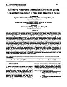
IJCA Special Issue on “Network Security and Cryptography” NSC, 2011 is connected to a router through internal an IP router and the router is connected to internet through an external IP router. The server is connected to the L3 switch through mirror port to observe the traffic activity to the switch. Another LAN of 350 nodes is connected to other VLANs through five L3 and L2 switches and three routers. The attacks are launched within our testbed as well as from another LAN through the internet. In launching attacks within testbed, nodes of one VLAN are attacked from nodes of another VLAN and also the same VLAN. Normal traffic is created within our testbed in restricted condition after disconnecting another LAN. The traffic activities to our testbed are observed in the computer connected to the mirror port. A diagram of the testbed is shown in Figure 1.
certain time interval between source and destination hosts. All traffic belonging to a particular flow has a set of common properties. The NetFlow protocol (IPFIX standard) [36,37] provides a summarization of information about the router or switch traffic. Network flow is identified by source and destination IP addresses as well as by port numbers. [39] is a simple protocol that exports flow records of fixed size (48 bytes in total). To identify a flow uniquely, NetFlow also uses several fields, viz., types of protocols and types of services (ToS) from IP header, and the input logical interface of the router or the switch. Table 6. Packet level window-based features Sl No.
Features
1
count-destconn
2
count-srcconn
3
count-servsrc-conn
4
count-servdest-conn
Description Number of frames to unique destination IP addresses inside the network in the last N connection from the same source. Number of frames from unique source IP addresses inside the network in the last N connection to the same destination Number of frames from the source IP to the same destination port in the last N connection. Number of frames to the destination IP using same source port in the last N connection.
Table 7. Packet level content based features Sl No.
Figure 1: Testbed The packet level network traffic were captured by using open source software gulp[33]. Gulp has the ability to read directly from the network and decaptulate the packets. The packets were analyzed using the open source packet analyzing software wireshark [34]. The raw packet data were preprocessed and filtered before extracting and constructing new features. In packet level network traffic, 45 types of features were extracted. To extract these features we used open source tool tcptrace [35], C programs and perl script. These features are classified as basic, time-based, window-based and content-based features. The lists of features are given in Table 5-8. Table 5. Packet level time-based features Sl No.
2
count-src
3
countserv-src
Description Number of frames to unique destination IP addresses inside the network in the last T seconds from the same source. Number of frames from unique source IP addresses inside the network in the last T seconds to the same destination. Number of frames from the source IP to the same destination port in the last T seconds.
countserv-dest
Number of frames to the destination IP using same source port in the last T seconds.
1
4
Features count-dest
1
Features num packet src dst
Description The number of packets owing from the source to destination The number of packets owing from destination to source
2
num packet dst src
3
num acks src dst
4
num acks dst src
5
num bytes src dst
6
num bytes dst src
7
num retransmit src dst
8
num retransmit dst src
9
num pushed src dst
10
num pushed dst src
11
num SYNs src dst
The number of bytes owing from destination to source The number of retransmitted packets owing from source to destination The number of retransmitted packets owing from destination to source The number of pushed packets owing from source to destination The number of pushed packets owing from destination to source The number of SYN packets owing from source to destination
12
num FINs src dst
The number of FIN packets owing from source to destination
The number of acknowledgement packets owing from source to destination The number of acknowledgement packets owing from destination to source The number of bytes owing from source to destination
The network flow is a unidirectional sequence of packets passing through an observation point in the network during a
24
IJCA Special Issue on “Network Security and Cryptography” NSC, 2011 13
num SYNs dst src
The number of SYN packets owing from destination to source
14
num FINs dst src
The number of FIN packets owing from destination to source
15
connection status Status of the connection (0-Completed, 1-Not completed; 2- Reset) (discrete) Table 8. Packet level basic features Features Description
Sl No.
1
Time delta
Time since occurrence of first frame
2
Frame no.
Frame number
3
Frame length
Length of the frame
4
Capture length
Captured frame length
5
Header length
Header length of the packet
6
Fragment offset
Fragment offset value
7
ttl
Time to live
8
Protocol
Protocol of layer 3- IP, TCP, UDP
9
Src IP
Source IP address
10
Dest IP
Destination IP address
11
Src port
Source port of machine
12
Dest port
Destination port of machine
13
Seq. no.
Sequence number
14
CWR
Congestion Window Record
15
ECN
Explicit Congestion Notification
16
URG
Urgent TCP flag
17
ACK
Acknowledgement flag
18
PSH
Push flag
19
RST
Reset flag
20
SYN
Syn flag
21
FIN
Fin flag
22
Window size
Sliding window size
The flows are stored in router or the switch cache and exported to a collector under the following constraints (i) flows that have been idle for a specified time are expired where default setting of specified time is 15 seconds, or the user can configure this time to be between 10 to 600 sec., (ii) flows lived longer than 30 minutes are expired, (iii) if the cache reaches its maximum size, a number of heuristic expiry functions are applied to export flows, and (iv) a TCP connection has finished with flag FIN or RST. A flow collector tool, viz., nfdump [32] receives flow records from the flow exporter and stores them in a form suitable for further monitoring or analysis. A flow record is the information stored in the flow exporter cache. A flow exporter
protocol defines how expired flows are transferred by the exporter to the collector. The information exported to the collector is referred to as flow record. NetFlow version 5 [33] is a simple protocol that exports flow records of fixed size (48 bytes in total). To identify a flow uniquely, NetFlow also uses several fields, viz., types of protocols and types of services (ToS) from IP header, and the input logical interface of the router or the switch. The flows are stored in router or the switch cache and exported to a collector under the following constraints (i) flows that have been idle for a specified time are expired where default setting of specified time is 15 seconds, or the user can configure this time to be between 10 to 600 sec., (ii) flows lived longer than 30 minutes are expired, (iii) if the cache reaches its maximum size, a number of heuristic expiry functions are applied to export flows, and (iv) a TCP connection has finished with flag FIN or RST. Network flow is identified by source and destination IP addresses as well as by port numbers. [39] is a simple protocol A flow collector tool, viz., nfdump [32] receives flow records from the flow exporter and stores them in a form suitable for further monitoring or analysis. A flow record is the information stored in the flow exporter cache. A flow exporter protocol defines how expired flows are transferred by the exporter to the collector. The information exported to the collector is referred to as flow record. NetFlow version 5 [33] is a simple protocol that exports flow records of fixed size (48 bytes in total). We used the NetFlow version 5 protocol to export flow records and used nfdump to receive flow records. All data are stored on disk before analyzing. This separates the process of storing and analyzing the data. The data is organized in a time based fashion. Nfdump has a flow record capturing daemon process nfcapd which reads data from the network and stores the data into files. Automatically, in every n minutes, typically 5 minutes, nfcapd rotates and renames each output file with time stamp nfcapd, YYYYMMddhhmm, e.g., nfcapd, 201012110845 contains data from December 11th 2010 08:45 onward. Based on a 5 minutes time interval, this stores results in 288 files per day. Analysis of the data is done by concatenating several files for a single run. The output is stored either in ASCII or in binary into a file and it is ready to be processed again with the same tool. We used C programs to filter the captured data to extract new features. Unnecessary parameters were removed and the retained parameters were flow-start, duration, protocol, sourceIP, source-Port, destination-IP, destination-Port, flags, ToS, bytes, packets-per-second (pps), bits-per-second (bps) and bytesper-packet (Bps). Network traffic corresponding to attack and normal traffic was gathered using our local network within a 4 week period. We collected 1,48,712 flow records of 16 attack types and normal records. The extracted features were of 23 types and were classified into three groups of features: (i) basic, (ii) time-window based, and (iii) connection based features. The list of features is given in Table 9-11. Table 9. Flow level time-window features Sl No.
1 2
Features
count-dest
count-src
Description
Number of flows to unique destination IP addresses inside the network in the last T seconds from the same source. Number of flows from unique source IP addresses inside the network in the last T
25
IJCA Special Issue on “Network Security and Cryptography” NSC, 2011
3 4
countserv-src countserv-dest
seconds to the same destination. Number of flows from the source IP to the same destination port in the last T seconds. Number of flows to the destination IP using same source port in the last T seconds.
Table 10. Flow level Connection based features Sl No.
1
Features count-destconn
2
count-srcconn
3
count-servsrc-conn count-servdest-conn
4
Description Number of flows to unique destination IP addresses inside the network in the last N flows from the same source. Number of flows from unique source IP addresses inside the network in the last N flows to the same destination. Number of flows from the source IP to the same destination port in the last N flows. Number of flows to the destination IP using same source port in the last N flows..
Table 11. Flow level basic features Sl No.
1
Features Duration
Description Length of the flow (in seconds)
2
Protocol-type
Type of protocols- TCP, UDP, ICMP
3
Src IP
Source node IP address
4
Dest IP
Destination IP address
5
Src port
Source port
6
Dest port
Destination port
7
ToS
Type of service
8
URG
Urgent flag of TCP header
9
ACK
Acknowledgement flag
10
PSH
Push flag
11
RST
Reset flag
12
SYN
SYN flag
13
FIN
FIN flag
14
Source byte
Number of data bytes transfer from source IP to destination IP
15
Land
Same source IP/source port are equal to Destination IP/Destination port
and 3 categorical attributes). Each record is labeled as either normal or one specific kind of attack. Each dataset contains 22 types of attacks. The two datasets of KDD Cup 1999 : (i) Corrected KDD, and (ii) 10% KDD are given in Table 12. Table 12. KDD Cup 1999 Dataset Datasets
Normal
Attacks
Total
Corrected KDD
60593
250436
311029
10% KDD
97278
396743
494021
4.1.3 NSL-KDD Dataset NSL-KDD [14] is a network-based intrusion dataset. It is a filtered version of KDD Cup 1999 intrusion detection benchmark dataset. In the KDD Cup 1999 dataset, there are huge number of redundant records, which can cause the learning algorithms to be biased towards the frequent records. To solve this issue, one copy of each record was kept in the NSL-KDD dataset. The two datasets of NSL-KDD: (i) KDDTrain+, and (ii) KDDTest+ are shown in Table 13. Table 13. NSL-KDD Dataset Datasets KDDTrain KDDTest
+
+
Normal
Attacks
Total
67343
58630
125973
9710
12834
22544
4.2 Performance measures
4.1.2 KDD Cup 1999 Dataset The proposed method was tested on datasets available in the KDD Cup 1999 intrusion detection benchmark datasets [13]. Each record of the datasets represents a connection between two network hosts according to network protocols and is described by 41 attributes (38 continuous or discrete numerical attributes
Evaluation of performance of a clustering model is based on the counts of test records correctly and incorrectly predicted by the model. These counts are tabulated in a table known as a confusion matrix [40]. A confusion matrix summarizes number of instances predicted correctly or incorrectly by a classification model and it is given in Table 14. Table 14. Confusion matrix for binary classification
+ Actual Class
-
Predicted Class + TP FN FP
TN
The following terminology is often used when referring the counts tabulated in the confusion matrix. True positive (TP), which corresponds to the number of positive examples correctly predicted by the classification model. False negative (FN), which corresponds to the number of positive examples wrongly predicted as negative by the classification model. False positive (FP), which corresponds to the number of negative examples wrongly predicted as positive by the classification model. True negative (TN), which corresponds to the number of negative examples correctly predicted by the classification model. The counts in a confusion matrix can also be expressed in terms of percentages. True positive rate (TPR) is defined as the fraction of positive examples predicted correctly by the model, i.e., TPR = TP/(TP + FN). (6) Similarly, the true negative rate (TNR) is defined as the fraction of negative examples predicted correctly by the model, i.e.,
26
IJCA Special Issue on “Network Security and Cryptography” NSC, 2011 TNR = TN/(TN + FP). (7) The false positive rate (FPR) is the fraction of negative examples predicted as positive class, i.e., FPR = FP/(TN + FP). (8) Finally, the false negative rate (FNR) is the fraction of positive examples predicted as negative class, i.e., FNR = FN/(TP + FN). (9) Detection Rate: The detection rate (DR) is defined as the number of intrusion instances detected by the system divided by the total number of intrusion instances present in the test dataset. In confusion matrix, detection rate can be represented by TNR.
4.3 Experimental results Three datasets viz. (i) Real Life Network Intrusion Dataset, (ii) KDD Cup 1999 Dataset and (iii) NSL-KDD dataset, and are used to evaluate the performance of our algorithm. We experimented as each of its dataset using two distinct approaches (i) over full feature space, k-point-1 algorithm and (ii) over reduced feature space (identifying relevant feature specific to a particular class, while using approach (ii), k-point-2 algorithm. Our experiments carried out after preprocessing of the above three datasets. Each preprocessing has two phases: data normalization and feature reduction phases. After all attribute values of each data set are scaled to the range [0-1] by dividing every attribute value by its own maximum value, we utilize the mutual information based feature selection algorithm [30] to select important features for each dataset. The performance evaluation over the dataset and its preprocessed dataset are presented next.
4.3.1 Results on Real Life Network Intrusion Dataset using k-point-1 Algorithm The confusion matrices for two dataset Packet-level and Flowlevel of our Real Life Network Intrusion Dataset are given in Table 15 and 16. On Packet Level dataset, the DR for intrusion records is 99.29%, TPR for normal records is 98.89% and FPR for normal records is 0.71%. Similarly, on Flow Level dataset, the DR for intrusion records is 99.53%, TPR for normal records is 99.11% and FPR for normal records is 0.47%. Table 15. Confusion matrix for Packet level dataset using k-point-1 algorithm
for dataset Packet-level is given in Table 17. The DR for intrusion records is 99.54%, TPR for normal records is 98.25% and FPR for normal records is 0.49%. Similarly, in data preprocessing and feature selection of dataset Flow-level, eight number features [8, 9, 16, 17, 18, 20, 31, 34] are reduced. The confusion matrices for dataset Flow-level is given in Table 18. The DR for intrusion records is 99.53%, TPR for normal records is 99.11% and FPR for normal records is 0.47%. Table 17. Confusion matrix for Packet level dataset using k-point-2 algorithm Predicted Class
Actual Class
Normal Attack Sum
Actual Class
Normal Attack Sum
Attack
Sum
31135 1411 32546
350 197287 197637
31485 198698 230183
Table 16. Confusion matrix for Flow level dataset using k-point-1 algorithm
Actual Class
Normal Attack Sum
Attack
Sum
32325 546 32871
291 115550 115841
32616 116096 148712
4.3.2 Results on Real Life Network Intrusion Dataset using k-point-2 Algorithm In data preprocessing and feature selection of dataset Packetlevel, sixteen numbers of features [7, 8, 9, 11, 15, 16, 17, 18, 19, 20, 25, 26, 29, 30, 31, 34] are reduced. The confusion matrices
Sum
30935 911 31846
550 197787 198337
31485 198698 230183
Predicted Class
Actual Class
Normal Attack Sum
Normal
Attack
Sum
32025 246 32271
591 115850 116441
32616 116096 148712
4.3.3 Results on KDD Cup 1999 Dataset using kpoint-1 Algorithm The confusion matrices for two dataset Corrected KDD and 10 percent KDD of KDD Cup 1999 Dataset are given in Table 19 and 20. On Corrected KDD dataset, the DR for intrusion records is 97.55%, TPR for normal records is 90.01% and FPR for normal records is 2.45%. Similarly, on 10 percent KDD dataset, the DR for intrusion records is 95.75%, TPR for normal records is 94.76% and FPR for normal records is 4.25%. Table 19. Confusion matrix for Corrected KDD dataset using k-point-1 algorithm Predicted Class
Actual Class
Normal Attack Sum
Normal
Attack
Sum
54540 6135 60675
6053 244301 250354
60593 250436 311029
Table 20. Confusion matrix for 10 percent KDD dataset using k-point-1 algorithm Predicted Class
Predicted Class Normal
Attack
Table 18. Confusion matrix for Flow level dataset using k-point-2 algorithm
Predicted Class Normal
Normal
Actual Class
Normal Attack Sum
Normal
Attack
Sum
92180 16846 109026
5098 379897 384995
97278 396743 494021
4.3.4 Results on KDD Cup 1999 Dataset using kpoint-2 Algorithm In data preprocessing and feature selection, fourteen numbers of features [8, 9, 11, 16, 17, 18, 19, 20, 25, 26, 29, 30, 31, 34] are reduced from the two dataset Corrected KDD and 10 percent KDD. The confusion matrices for the two dataset Corrected
27
IJCA Special Issue on “Network Security and Cryptography” NSC, 2011 KDD and 10 percent KDD of KDD Cup 1999 dataset are given in Table 21 and 22. Table 21. Confusion matrix for Corrected KDD dataset using k-point-2 algorithm
57413 58630 Attack 1217 64245 61728 125973 Sum Table 26. Confusion matrix for KDDTest+ dataset using k-point-2 algorithm
Predicted Class
Actual Class
Normal Attack Sum
Predicted Class
Normal
Attack
Sum
54540 5635 60175
6053 244801 250854
60593 250436 311029
Table 22. Confusion matrix for 10 percent KDD dataset using k-point-2 algorithm Predicted Class
Actual Class
Normal Attack Sum
Normal
Attack
Sum
92280 16846 109126
4998 16846 384895
97278 396743 494021
4.3.5 Results on NSL-KDD Dataset using k-point-1 Algorithm The confusion matrices for two datasets KDDTrain+ and KDDTest+ of NSL-KDD Dataset are given in Table 23 and 24. On KDDTrain+ dataset, the DR for intrusion records is 97.65%, TPR for normal records is 93.89% and FPR for normal records is 2.35%. Similarly, on KDDTest+ dataset, the DR for intrusion records is 98.88%, TPR for normal records is 96.55% and FPR for normal records is 1.12%. Table 23. Confusion matrix for KDDTrain+ dataset using k-point-1 algorithm Predicted Class
Actual Class
Normal Attack Sum
Normal
Attack
Sum
63228 1377 64445
4115 57413 61528
67343 58630 125973
Table 24. Confusion matrix for KDDTest+ dataset using k-point-1 algorithm Predicted Class
Actual Class
Normal Attack Sum
Normal
Attack
Sum
9375 144 9519
335 12690 13025
9710 12834 22544
4.3.6 Results on NSL-KDD Dataset using k-point-2 Algorithm Ten numbers of features [8, 9, 11, 18, 19, 20, 25, 26, 30, 34] are scaled down in data preprocessing and feature selection for two datasets KDDTrain+ and KDDTest+ of NSL-KDD. The confusion matrices for the two datasets KDDTrain+ and KDDTest+ of NSL-KDD Dataset are given in Table 25 and 26. Table 25. Confusion matrix for KDDTrain+ dataset using k-point-2 algorithm Predicted Class Actual Class
Normal
Normal
Attack
63028
4315
Actual Class
Normal Attack Sum
Normal
Attack
Sum
9275 104 9379
435 12730 13165
9710 12834 22544
On KDDTrain+ dataset, the DR for intrusion records is 97.92%, and TPR and FPR for normal records are 93.59% and 2.08% respectively. Similarly, on KDDTest+ dataset, the DR for intrusion records is 99.19%, and TPR and FPR for normal records are 95.52% and 0.81% respectively.
4.3.7 Comparison of Results The summarized results over the three distinguished datasets are made for detection rate (DR) on intrusive records, TPR and FPR over normal records for the datasets. The comparison results for the datasets for k-point-1 algorithm are presented in Table 27. Table 27. Experimental Results of k-point-1 Algorithm Data sets
Total
Attacks
Normal
Detection Rate (%)
TPR (%)
FPR (%)
Corrected KDD
311029
250436
60593
97.55
90.01
2.45
10% KDD
494021
396743
97278
95.75
94.76
4.25
KDDTrain+
125973
58630
67343
97.65
93.89
2.35
KDDTest+
22544
12834
9710
98.88
96.55
1.12
Packet Level
230183
198698
31485
99.29
98.89
0.71
Flow Level
148712
116096
32616
99.53
99.11
0.47
Similarly, the summarized results using k-point-2 algorithm are made for detection rate (DR) on intrusive records, TPR and FPR over normal records for the preprocessed datasets. The comparison results are presented in Table 28. Table 28. Experimental Results of k-point-2 Algorithm Data sets
Total
Attacks
Normal
Detection Rate (%)
TPR (%)
FPR (%)
Corrected KDD
311029
250436
60593
97.75
90.01
2.25
10% KDD
494021
396743
97278
95.75
94.86
4.25
KDDTrain+
125973
58630
67343
97.92
93.59
2.08
KDDTest+
22544
12834
9710
99.19
95.52
0.81
Packet Level
230183
198698
31485
99.54
98.25
0.49
Flow Level
148712
116096
32616
99.79
98.19
0.21
Sum 67343
28
IJCA Special Issue on “Network Security and Cryptography” NSC, 2011
4.3.8 Performance Comparisons The performance of k-point-1 algorithm is compared with other four unsupervised anomaly-based intrusion detection algorithms: fpMAFIA [8], K-NN [6], fixed width clustering [6] and Modified Clustering-TV [16]. The comparison results of performance over Corrected KDD dataset for all these algorithms are shown in Table 29. In the performance comparison, detection rate for intrusion instances by k-point algorithms are maximum. Table 29. Comparison with Unsupervised Techniques on Corrected KDD Algorithm fpMAFIA [8]
Detection Rate (%) 86.70
K-NN [6]
89.95
Fixed width clustering [6] Modified Clustering-TV [16] k-point-1 algorithm k-point-2 algorithm
94.00 97.30 97.55 97.75
5. CONCLUSION AND FUTURE WORKS In this paper we have provided a clustering based method and applied it in unsupervised anomaly based network intrusion detection. We have developed the clustering method by building normal behavior model from unlabeled dataset. We evaluated the anomaly detection approach by applying it to network intrusion detection on evaluated benchmark intrusion dataset as well as on real life network intrusion dataset captured in local network and compared it to existing method of unsupervised network anomaly detection. However, the framework presented for network intrusion detection can be applied for broader classification problems. For example, the method can be applied for error detection in large datasets considering maximum instances as normal compared to erroneous instances.
6. ACKNOWLEDGEMENT We acknowledge the reviewers and the Department of Information Technology, Ministry of Information Technology, Government of India for funding this research work.
7. REFERENCES [1] Bace, R. and Mell, P. (2001). Intrusion detection systems. NIST Special Publications SP 800, U S Department of Defence, 31 November 2001. [2] Lee, W. and Stolfo, S. J. (1998) Data mining approaches for intrusion detection. Proceedings of the 7th conference on USENIX Security Symposium-Volume 7, San Antonio, Texas, USA, Jan., pp. 6–6. USENIX. [3] Roesch, M. (1999) Snort-lightweight intrusion detection for networks. Proceedings of the 13th USENIX conference on System administration, Seattle, Washington, Nov., pp. 229– 238. USENIX. [4] Portnoy, L., Eskin, E., and Stolfo, S. J. (2001) Intrusion detection with unlabeled data using clustering. In Proc. of the ACM CSS workshop DMSA-2001, Philadelphia PA, November 8, pp. 5–8. ACM. [5] Daniel, B., Julia, C., Sushil, J., and Ningning, W. (2001) Adam: a testbed for exploring the use of data mining in intrusion detection. SIGMOD Rec., 30, 15–24.
[6] Eskin, E., Arnold, A., Prerau, M., Portnoy, L., and Stolfo, S. (2002) A geometric framework for unsupervised anomaly detection. Applications of Data Mining in Computer Security, Norwell, MA, USA, Dec., pp. 78–100. Kluwer Academic Publishers. [7] Smith, R., Bivens, A., Embrechts, M., Palagiri, C., and Szymanski, B. (2002) Clustering approaches for anomaly based intrusion detection. Proc. of Walter Lincoln Hawkins Graduate Research Conference 2002, New York, USA, October. [8] Leung, K. and Leckie, C. (2005) Unsupervised anomaly detection in network intrusion detection using clusters. Proc. of 28 Australasian conference on Computer Science Volume 38, Newcastle, NSW, Australia, January/February, pp. 333–342. Australian Computer Society, Inc. Darlinghurst. [9] Leon, E., Nasraoui, O., and Gomez, J. (2004) Anomaly detection based on unsupervised niche clustering with application to network intrusion detection. IEEE Congres on Evolutionary Computation, 1, 502–508. [10] Chimphlee, W., Abdullah, A. H., Sap, M. N. M.,Chimphlee, S., and Srinoy, S. (2005) Unsupervised clustering methods for identifying rare events in anomaly detection. Proc. of World Academy of Science, Engineering and Technology, October. [11] Zhong, S., Khoshgoftaar, T., and Seliya, N. Clusteringbased network intrusion detection. Int’nl J of Reliability, Quality and Safety Engineering,14. [12] Zhang, C., Zhang, G., and Sun, S. (2009) A mixed unsupervised clustering-based intrusion detection. Proc. of 3rd International Conference on Genetic and Evolutionary Computing, WGEC 2009, Gulin, China, 14-17 October. IEEE Computer Society. [13] Hettich, S. and Bay, S. D. (1999). The uci kdd archive. Irvine, CA:University of California, Department of Information and Computer Science, http://kdd.ics.uci.edu. [14] Tavallaee, M., Bagheri, E., Lu, W., and Ghorbani, A. A. (2009). A detailed analysis of the kdd cup 99 data set. Availble on: http://nsl.cs.unb.ca/NSL-KDD/. [15] Eskin, E. (2000) Anomaly detection over noisy data using learned probability distributions. Proceedings of the 7th International Conference on Machine Learning, Stanford University, Stanford, CA, USA, June 29-July 2, pp. 255– 262. Morgan Kaufmann Publishers Inc. [16] 16. Oldmeadow, J., Ravinutala, S., and Leckie, C. (2004) Adaptive clustering for network intrusion detection. In Proc. of the PAKDD 2004, Sydney, Australia, May 26-28, pp. 255–259. LNCS 3056 Springer 2004, ISBN 3-54022064-X. [17] Guan, Y., Ghorbani, A., and Belacel, N. (2003) Ymeans: A clustering method for intrusion detection. Proc. of the Canadian Conference on Electrical and Computer Engineering, Montreal, Quebec, Canada, May 4-7. [18] Lu,W. and Traore, I. Unsupervised anomaly detection using an evolutionary extension of k-means algorithm. Int. J. Information and Computer Security, 2. [19] Nagesh, H. S., Goil, S., and Choudhary, A. N. (2000) A scalable parallel subspace clustering algorithm for massive data sets. Proc. of the ICPP 2000, Toronto, Canada, 21-24 August 477. IEEE Computer Society. [20] Burbeck, K. and Nadjm-Tehrani, S. (2005) Adwice anomaly detection with real-time incremental clustering.
29
IJCA Special Issue on “Network Security and Cryptography” NSC, 2011
[21]
[22]
[23]
[24]
[25]
[26]
[27]
[28]
Proceedings of Information Security and Cryptology ICISC 2004, Berlin , Germany, May, pp. 407–424. Springer Berlin / Heidelberg. Zhang, T., Ramakrishnan, R., and Livny, M. (1996) Birch: an efficient data clustering method for very large databases. Proc. of the 1996 ACM SIGMOD, Montreal, Quebec, Canada, June 4-6, pp. 103–114. ACM Press. Proto, A., Alexandre, L. A., Batista, M. L., Oliveira, I. L., and Cansian, A. M. Statistical model applied to netflow for network intrusion detection. LNCS, 6480. Diaz-Verdejo, P. G.-T. J., Macia-Fernandez, G., and Vazquez, E. Anomaly-based network intrusion detection: Techniques, systems and challenges. Computers & Security, 28. Gogoi, P., Borah, B., and Bhattacharyya, D. K. Anomaly detection analysis of intrusion data using supervised & unsupervised approach. Journal of Convergence Information Technology, 5. Gogoi, P., Bhattacharyya, D. K., Borah, B., and Kalita, J. K. A survey of outlier detection methods in network anomaly identification. The Computer Journal, 54. Cha, S.-H. (2007) Comprehensive survey on distance/ similarity measures between probability density functions. nternational Journal of Mathematical Models and Methods in Applied Science, 1 (4), 300–307. Boriah, S., Chandola, V., and Kumar, V. (2008) Similarity measures for categorical data: A comparative evaluation. Proceedings of the 8th SIAM International Conference on Data Mining, Atlanta, Georgia, USA, Apr., pp. 243–254. Society for Industrial and Applied Mathematics(SIAM). T. S. Chou and L. J. K. K. Yen, “Network intrusion detection design using feature selection of soft computing paradigms,” International Journal of computational Intelligence, vol. 4, pp. 196–208, 2008.
[29] S. Mukkamala and A. H. Sung, “Significant feature selection using computational intelligent techniques for intrusion detection,” Advanced Method for Knowledge Discovery from Complex Data, vol. Part II, pp. 285–306, 2005. [30] F. Amiri, M. M. R. Yousefi, C. Lucas, A. Shakery, and N. Yazdani, “Mutual information-based feature selection for intrusion detection systems,” Journal of Network and Computer Applications, vol. 34, pp. 1184-1199, 2011. [31] H.G. Kayacik, A.N. Zincir-Heywood, and M.I. Heywood, “Selecting Features for Intrusion Detection: A Feature Relevance Analysis on KDD 99 Intrusion Detection Datasets”, In Proceedings of the 3rd Annual Conference on Privacy, Security and Trust (PST-2005), Oct., 2005. [32] Mixter (2003). Attacks tools and information. http://packetstormsecurity.nl/index.html. [33] Satten, C. (2008). Lossless gigabit remote packet capture with linux. http://staff.washington.edu/corey/gulp/, University of Washington Network Systems. [34] (2009). Wireshark. http://www.wireshark.org/. [35] Osterman, S. (2009). Tcptrace. http://www.tcptrace.org. [36] Quittek, J., Zseby, T., Claise, B., and Zender, S. (2004). Rfc 3917: Requirements for ipflow information export: Ipfix, hawthorn victoria. http://www.ietf.org/rfc/rfc3917.txt. [37] Claise, B. (2004). Rfc 3954: Cisco systems netflow services export version 9. http://www.ietf.org/rfc/rfc3954.txt. [38] Haag, P. (2010). Nfdump & nfsen. http://nfdump.sourceforge.net/. [39] Cisco.com (2010). Cisco ios netflow configuration guide, release 12.4. http://www.cisco.com. [40] Tan, P.-N., Steinbach, M., and Kumar, V. (2009) Introduction to Data Mining. Pearson Education, Inc., Newyork, USA.
30