2008 American Control Conference Westin Seattle Hotel, Seattle, Washington, USA June 11-13, 2008
FrC15.5
Robust H∞ Performance Analysis for Continuous-Time Networked Control Systems Xun-Lin Zhu and Guang-Hong Yang Abstract— This paper studies the problems of robust H∞ performance analysis and controller design for continuous-time networked control systems (NCSs). A new type of Lyapunov functionals is exploited to derive sufficient conditions for guaranteeing the robust exponential stability and H∞ performance of the considered system, and robust H∞ controller design is presented. It is shown that the newly obtained result is less conservative than the existing corresponding ones. Meanwhile, by using a method of eliminating redundant variables, the computation complexity is reduced. Numerical examples are given to illustrate the effectiveness of the proposed methods.
I. INTRODUCTION Networks have received increasing attention in recent years because of the popularization and advantages of using network cables in control systems. The network itself is a dynamic system and induces possible delays via network communication due to limited bandwidth. A realistic networked control system design should take the communication delays into account, since the delays are widely known to degrade the performance of the control system. In the past decade, the control problem of networked systems with time-delays has received increasing attention. [1] studied the problem of packet dropout and transmission delays induced by communication network of NCSs in both continuous time and discrete time cases. By using the Lyapunov-Razumikhin function techniques, [2] obtained the delay-dependent condition on the stabilization of NCSs in terms of linear matrix inequalities (LMIs). The admissible upper bounds of data packet loss and delays can be computed by using the quasi-convex optimization algorithm. [3] discussed the design of robust H∞ controllers for uncertain NCSs with both the network-induced delay and data dropout. [4] was concerned with the controller design of NCSs. A This work was supported in part by Program for New Century Excellent Talents in University (NCET-04-0283), the Funds for Creative Research Groups of China (No. 60521003), Program for Changjiang Scholars and Innovative Research Team in University (No. IRT0421), the State Key Program of National Natural Science of China (Grant No. 60534010), the Funds of National Science of China (Grant No. 60674021) and the Funds of PhD program of MOE, China (Grant No. 20060145019), the 111 Project (B08015). Xun-Lin Zhu is with the College of Information Science and Engineering, Northeastern University, Shenyang, Liaoning, 110004, China. He is also with the School of Computer and Communication Engineering, Zhengzhou University of Light Industry, Zhengzhou, Henan, 450002, China.
new model of NCSs was provided under consideration of both the network-induced delay and the data packet dropout in the transmission, and a controller design method was proposed based on a delay-dependent approach. [5] studied the stabilization problem of NCSs where the main focus was the packet-loss issue. Two types of packet-loss processes were considered. One was the arbitrary packet-loss process, the other was the Markovian packet-loss process. In this paper, the problem of robust H∞ performance analysis for continuous-time NCSs is investigated. The objective is to seek for improved LMI-based conditions for ensuring larger delay bounds and better H∞ performance. A new type of Lyapunov functionals is proposed, and new delay-dependent criteria for the H∞ performance analysis are derived. Using these criteria, an upper bound of timedelay can be obtained such that the considered system is robustly exponentially stable with a prescribed H∞ performance bound. It is shown that the new result is less conservative than the existing corresponding ones. Meanwhile, by using a method of eliminating redundant variables, the computational complexity is also reduced. The organization of this paper is as follows. Section 2 models an NCS with data packet dropout and transmission delays as a linear system with time-varying input delay. Section 3 presents H∞ performance analysis, controller design, and a method of eliminating redundant variables. It proves that the newly obtained stability condition is less conservative than some latest results. Three numerical examples are given to show the effectiveness of the criteria in Section 4, and finally conclusions are stated in Section 5. II. SYSTEM DESCRIPTION Throughout this paper, we assume that the sensor is clockdriven, the controller and actuator are event-driven and hold the latest data, h is the length of sampling period. Single packet transmission is considered throughout this paper. The actuator and the sensor are connected through a communication network with finite bandwidth. Data packet dropout and disordering in an NCS are unavoidable because of limited bandwidth. An NCS with the possibility of dropping data packet and disordering can be described as in Figure 1. The model presented here is the same as that in [3]: x(t) ˙ = Ax(t) + Bu(t) + Bω ω (t), x(t) = φ (t), t ∈ [t1 − h2 , t1 ], z(t) = Cx(t) + Du(t),
[email protected]
Guang-Hong Yang is with the College of Information Science and Engineering, Northeastern University, Shenyang, Liaoning, 110004, China. He is also with the Key Laboratory of Integrated Automation of Process Industry, Ministry of Education, Northeastern University, Shenyang 110004, China. Corresponding author.
[email protected],
yang
[email protected]
978-1-4244-2079-7/08/$25.00 ©2008 AACC.
(1) (2) (3)
where x(t) ∈ ℜn is the state vector, u(t) ∈ ℜ p is the control input vector, z(t) ∈ ℜq is controlled output, ω (t) ∈ L2 [t1 , ∞)
5204
where
Fig. 1.
Λ1 =
An NCS with data packet dropout and transmission delays
t ∈ {ik h + τk , k = 1, 2, · · · },
(4)
where time-delay τk denotes the time from the instant ik h when the sensor node samples sensor data from a plant to the instant tk when the actuator receives the control signal, i.e., τk = tk − ik h, and τk = τksc + τkca , where τksc is the sensorto-controller time-delay of x(ik h) , and τkca is the controllerto-actuator time-delay of u(i ¯ k h − τksc ). Obviously, ∪∞ k=1 [ik h + τk , ik+1 h + τk+1 ) = [t1 , ∞), t1 ≥ 0. As pointed out in [3], under assumption: (ik+1 − ik )h + τk+1 ≤ h2 , k = 1, 2, · · · , 0 ≤ h1 ≤ τk , k = 1, 2, · · · ,
(5) (6)
where h1 , h2 are constants, then the system (1)-(4) can be rewritten as follows: x(t) ˙ = Ax(t) + BKx(t − d(t)) + Bω ω (t), x(t) = φ (t), t ∈ [t1 − h2 , t1 ] z(t) = Cx(t) + DKx(t − d(t)), 0 ≤h1 ≤ d(t) ≤ h2 ,
(7) (8) (9) (10)
where d(t) = t − ik h, t ∈ [ik h + τk , ik+1 h + τk+1 ), which denotes the time-varying delay in the control signal. Obviously, d(t) is not always differentiable in the interval [t1 , ∞]. In this paper, we analyze the robust H∞ performance of the closed-loop system (7)-(10). Remark 1. The above mentioned problem was also studied in [3]. In fact, many results of time-delay systems can be applied to deal with this problem, among them the result in [6] is one of the latest and it is listed as follows. Lemma 1. [6] For given scalars h1 , h2 (h2 > h1 ≥ 0) and a matrix K, the linear system (7)-(8) with time-varying delay d(t) satisfying (10) and Bω = 0 is asymptotically stable if there exist matrices P1 > 0, Si > 0, Qi ≥ 0, Yi , Ti , Vi (i = 1, 2), such that the following LMI holds: · ¸ Λ1 Λ2 Λ= < 0, (11) ∗ Λ3
Λ11 ∗ ∗ ∗ ∗
Λ12 Λ22 ∗ ∗ ∗
V1 V2 −Q1 ∗ ∗
−T1 −T2 0 −Q2 ∗
h2Y1 h2Y2 0 0 −h2 S1
h12 T1 h12 T2 0 0 0
∗
∗
∗
∗
∗
−h12 ∑ Si
2
,
i=1
Λ11 = P1 A + AT P1 + Q1 + Q2 +Y1 +Y1T , Λ12 = P1 (BK) +Y2T −Y1 + T1 −V1 , Λ22 =T2 + T2T −Y2 −Y2T −V2 −V2T , h12V1 AT (h2 S1 + h12 S2 ) h12V2 (BK)T (h2 S1 + h12 S2 ) 0 0 , Λ2 = 0 0 0 0 0 0 Λ3 = diag{−h12 S2 , − (h2 S1 + h12 S2 )}, h12 = h2 − h1 .
denotes the external perturbation, and t1 denotes the instant the actuator receives the 1st control signal. A, B, Bω , C, D are constant matrices of appropriate dimensions; xc is the delayed version of x, u is the delayed version of uc , and uc (t) = Kxc (t). Here, K is the state feedback gain matrix. Denote the instant the actuator receives the kth control signal as tk , and this control signal is based on the state of plant at the instant ik h, thus {i1 , i2 , i3 , · · · } ⊂ Z + , and u(t + ) = Kx(t − τk ),
III. MAIN RESULTS In this section, a new type of Lyapunov-Krasovskii functionals is proposed to derive new delay-dependent robust exponential stability criteria for the system (7)-(10) with a prescribed H∞ performance level. By eliminating redundant variables, a method for designing state feedback H∞ controllers is presented. A. H∞ performance analysis In the following, we will give new sufficient conditions which can ensure the exponential stability of NCS (7)-(10) with a prescribed H∞ performance bound. Lemma 2. For given scalars h1 , h2 (h2 > h1 ≥ 0), γ > 0, and a matrix K, the system (7)-(10) is exponentially stable with an H∞ norm bound γ if there exist n × n matrices Pi j , Pi j = PjiT (i, j = 1, 2, 3), P11 > 0, Qi ≥ 0, Zi ≥ 0, Ni , Si ≥ 0 (i = 1, 2), and matrices Mi (i = 1, 2, · · · , 9), such that Γ < 0, and
P11 P= ∗ ∗
P12 P22 ∗
· P13 Zi P23 ≥ 0, Hi = ∗ P33
(12)
Ni Si
¸ ≥ 0, (13)
where · ¸ Γ1 Γ2 Γ= − MA − A T M T , ∗ Γ 3 Γ11 Γ12 Γ13 P13 −P12 − P13 ∗ Γ22 0 0 0 −1 −1 ∗ Γ33 h12 S2 h12 (S1 + S2 ) Γ1 = ∗ , ∗ ∗ ∗ −Q1 − h−1 S 0 2 12 ∗ ∗ ∗ ∗ Γ55 T +CT C − h−1 S , Γ11 = Q1 + Q2 + h2 Z1 + h12 Z2 + P12 + P12 1 2 Γ12 = h2 N1 + h12 N2 + P11 , Γ13 = CT DK + h−1 2 S1 , Γ22 = h2 S1 + h12 S2 , −1 −1 Γ33 = (DK)T (DK) − h−1 2 S1 − h12 (S1 + S2 ) − h12 S2 , −1 Γ55 = −Q2 − h12 (S1 + S2 ),
5205
T P22 − h−1 P22 + P23 P23 2 N1 P P + P P13 12 12 13 −1 T −1 T Γ2 = h N Γ h 73 1 2 12 N2 T T T P23 P23 + P33 P33 − h−1 12 N2 T P22 − P23 Γ75 −P23 − P33 T T Γ73 = −h−1 12 (N1 + N2 ), T − P − P + h−1 (N T + N T ), Γ75 = −P22 − P23 23 33 1 2 12 −1 −1 Γ3 = diag{−h2 Z1 , − h−1 12 (Z1 + Z2 ), − h12 Z2 , £ T ¤ T M = £ M1 · · · M9T , ¤ A = A −I BK 0 0 0 0 0 Bω , h12 = h2 − h1 .
0 0 0 0 0
where
,
¸ Π1 Π2 Π= , ∗ Π3 Π11 Π12 P13 −P12 − P13 Π15 −1 ∗ Π22 h−1 Π25 12 S2 h12 (S1 + S2 ) T , ∗ ∗ Π 0 P Π1 = 33 23 T ∗ ∗ ∗ Π44 −P22 − P23 ∗ ∗ ∗ ∗ −h−1 2 Z1 T Π11 = Q1 + Q2 + h2 Z1 + h12 Z2 + P12 + P12 + (P11 + h2 N1 + h12 N2 )A + AT (P11 + h2 N1 + h12 N2 )T +CT C − h−1 2 S1 , Π12 = (P11 + h2 N1 + h12 N2 )BK +CT (DK) + h−1 2 S1 , T, Π15 = P22 + AT P12 − h−1 N 1 2 −1 −1 Π22 = (DK)T (DK) − h−1 2 S1 − h12 (S1 + S2 ) − h12 S2 , −1 T T Π25 = (BK) P12 + h2 N1 , Π33 = −Q1 − h−1 12 S2 , −1 Π44 =−Q2 − h12 (S1 + S2 ), Π16 P23 + AT P13 Π18 Π19 T Π26 (BK)T P13 + h−1 0 Π29 12 N2 −1 T T Π2 = P23 + P33 P33 − h12 N2 0 0 , Π46 −P23 − P33 0 0 TB 0 0 0 P12 ω T Π16 = P22 + P23 + A (P12 + P13 ), Π18 = (h2 N1 + h12 N2 + P11 )Bω , Π19 = AT (h2 S1 + h12 S2 ), T T Π26 = (BK)T (P12 + P13 ) − h−1 12 (N1 + N2 ), T Π29 = (BK) (h2 S1 + h12 S2 ), T − P − P + h−1 (N T + N T ), Π46 =−P22 − P23 23 33 1 2 12 −1 T + PT )B −h12 (Z1 + Z2 ) 0 (P12 0 13 ω TB 0 ∗ −h−1 P13 ω , 12 Z2 Π3 = Π89 ∗ ∗ −γ 2 I ∗ ∗ ∗ Π99 Π89 = BTω (h2 S1 + h12 S2 ), Π99 = −(h2 S1 + h12 S2 ), h12 = h2 − h1 .
− γ 2 I},
Proof: Construct a Lyapunov-Krasovskii functional as T x(t) x(t) Rt V (t) = t−h2 x(s)ds P t−h2 x(s)ds R t−h1 R t−h1 t−h2 x(s)ds t−h2 x(s)ds
Rt
2
+∑
i=1
R0
Rt
T t−hi x(s) Qi x(s)ds
Rt −h2 t+β
·
¸T
·
x(s) H1 x(s) ˙ · ¸T · R −h1 R t x(s) H2 + −h 2 t+β x(s) ˙
+
¸
(14)
x(s) dsd β x(s) ˙ ¸ x(s) dsd β , x(s) ˙
where P ≥ 0, Hi ≥ 0 (i = 1, 2) are defined in (13) and Qi ≥ 0 (i = 1, 2). Using the Cauchy-Schwarz inequality [7], and denoting ζ = [xT (t) x˙T (t) xT (t − d(t)) xT (t − h1 ) xT (t − h2 ) Rt R t−d(t) R t−h1 ( t−d(t) x(s)ds)T ( t−h2 x(s)ds)T ( t−d(t) x(s)ds)T ω T (t)]T ,
we can get
V˙ (t) + zT (t)z(t) − γ 2 ω T (t)ω (t) ≤ ζ T Γζ ,
(15)
which implies that ||z(t)||2 ≤ γ ||ω (t)||2 under zero initial condition. Similar to [3], we can prove the exponential stability of system (7)-(10). Thus, the proof is completed. Remark 2. In Lemma 2, a sufficient condition of exponential stability for the system (7)-(10) with an H∞ norm bound γ is given in terms of solutions to a set of LMIs. Different sufficient conditions are also given in [3] and [4]. The numerical comparison between Lemma 2 and the results in [3] and [4] will be given in Section 4. Note that the Lyapunov-Krasovskii functional (14) is more general, and lead to a less conservative stability condition than that in [6]. The details will be discussed in the sequel. By the elimination Lemma ([14], p.22), it is readily seen that if there exist matrices Mi (i = 1, 2, · · · , 9) that solve Γ < 0, if and only if · ¸ Γ1 Γ2 NA T NA < 0 (16) ∗ Γ3 holds, where NA denotes the full-rank matrix representations of the right annihilator of A . By the Schur complement, it yields that Π < 0, (17)
·
On the other hand, if Π < 0 holds, then it is very easy to see that Γ < 0 holds by taking M1 = −(P11 + h2 N1 + h12 N2 ), M2 = −(h2 S1 + h12 S2 ), T , M = −(P + P )T , T, M6 = −P12 M8 = −P13 7 12 13 M3 = M4 = M5 = M9 = 0. This implies that M3 , M4 , M5 , M9 are all redundant in Γ. Remark 3. From above analysis, it is shown that M6 is redundant when P12 = 0, M8 is redundant when P13 = 0, and M6 , M7 , M8 are redundant when P12 = P13 = 0 in Lemma 2. Thus, we have the following result for the H∞ performance analysis, which is equivalent to Lemma 2 and has fewer decision variables. Theorem 1. For given scalars h1 , h2 (h2 > h1 ≥ 0), γ > 0, and a matrix K, the system (7)-(10) is exponentially stable with an H∞ norm bound γ if there exist n × n matrices Pi j , Pi j = PjiT (i, j = 1, 2, 3), P11 > 0, Qi ≥ 0, Zi ≥ 0, Ni , Si ≥ 0 (i = 1, 2), and matrices Mi (i = 1, 2, · · · , 5), such that
5206
Θ < 0,
(18)
and
P11 P12 P13 P = ∗ P22 P23 ≥ 0, Hi = ∗ ∗ P33 where
·
Zi Ni ∗ Si
¸ ≥ 0 (i = 1, 2), (19)
·
¸ Γ1 Γ2 Θ= + Θ1 + ΘT1 , ∗ Γ3 £ T T Θ1 = £− M1 M2T 0 0 0 M3T M4T M ¤5 A = A −I BK 0 0 0 0 0 Bω ,
0
¤T
A,
From Theorem 1 and the equivalence of the inequality (17) and (18), we can derive the following stability conditions for the system (7)-(8). Corollary 1. For given scalar h1 , h2 (h2 > h1 ≥ 0) and matrix K, the linear system (7)-(8) with time-varying delay d(t) satisfying (10) and Bω = 0 is asymptotically stable if there exist matrices Pi j , Pi j = PjiT (i, j = 1, 2, 3), P11 > 0, Qi ≥ 0, Zi ≥ 0, Ni , Si ≥ 0 (i = 1, 2), such that the following LMIs hold: Ω < 0, (20) "
P= where
P11 ∗ ∗
P13 P23 P33
#
· ≥ 0, Hi =
Zi ∗
Ni Si
¸ ≥ 0 (i = 1, 2), (21)
¸ Ω1 Ω2 , ∗ Ω3 Ω11 Ω12 P13 −P12 − P13 Ω15 −1 ∗ Ω22 h−1 Ω25 12 S2 h12 (S1 + S2 ) T , ∗ Ω33 0 P23 Ω1 = ∗ T ∗ ∗ ∗ Ω44 −P22 − P23 ∗ ∗ ∗ ∗ −h−1 2 Z1 −1 T Ω11 = Q1 + Q2 + h2 Z1 + h12 Z2 + P12 + P12 − h2 S1 + (P11 + h2 N1 + h12 N2 )A + AT (P11 + h2 N1 + h12 N2 )T , Ω12 = (P11 + h2 N1 + h12 N2 )BK + h−1 2 S1 , T, Ω15 = P22 + AT P12 − h−1 N 1 2 −1 −1 Ω22 = −h−1 2 S1 − h12 (S1 + S2 ) − h12 S2 , T Ω25 = (BK)T P12 + h−1 2 N1 , −1 Ω33 = −Q1 − h12 S2 , Ω44 =−Q2 − h−1 12 (S1 + S2 ), Ω16 P23 + AT P13 Ω18 T Ω26 (BK)T P13 + h−1 Ω28 12 N2 −1 T T Ω2 = P23 + P33 P33 − h12 N2 0 , Ω46 −P23 − P33 0 0 0 0 Ω16 = P22 + P23 + AT (P12 + P13 ), Ω18 = AT (h2 S1 + h12 S2 ), T T Ω26 = (BK)T (P12 + P13 ) − h−1 12 (N1 + N2 ), T Ω28 = (BK) (h2 S1 + h12 S2 ), T − P − P + h−1 (N T + N T ), Ω46 = −P22 − P23 23 33 1 2 12 −1 Ω3 = diag{−h12 (Z1 + Z2 ), − h−1 12 Z2 , − (h2 S1 + h12 S2 )}, h12 = h2 − h1 . Ω=
·
P12 P22 ∗
0
h−1 12 I
12
0
0 ·
¸ I ∆4 and 0 I its transpose, respectively, then it is easy to see that Ω < 0 from Λ < 0 by taking P11 = P1 , P12 = P13 = P22 = P23 = P33 = 0 and Zi = ε I, Ni = 0 (i = 1, 2) with ε > 0 being sufficient small scalar. Remark 4. By Theorem 2, it proves theoretically that Corollary 1 is less conservative than Lemma 1. pre- and post-multiplying both sides of Λ by
and Γ1 , Γ2 , Γ3 are defined in Lemma 2 .
and
The comparison between Corollary 1 and Lemma 1 is given as follows. Theorem 2. If the LMI in Lemma 1 is feasible, the LMIs in Corollary 1 are also feasible. Proof: Denoting −h−1 0 0 0 2 I h−1 I −h−1 I h−1 I 0 2 12 12 ∆4 = (22) 0 0 −h−1 I 0
B. Robust performance analysis Next, consider the following system with parameter uncertainties given by .
x(t) = [A + ∆A(t)]x(t) + [B + ∆B(t)]u(t) + Bω ω (t),
(23)
where ∆A(t) and ∆B(t) denote the parameter uncertainties satisfying the following condition: £ ¤ £ ¤ ∆A(t) ∆B(t) = GF(t) Ea Eb , (24) where G, Ea and Eb are constant matrices of appropriate dimensions and F(t) is an unknown time-varying matrix, which is Lebesque measurable in t and satisfies F T (t)F(t) ≤ I, ∀ t ≥ 0.
(25)
In this case, from Theorem 1, (18) is substituted by £ ¤ ˜ Ea 0 Eb K 0 0 0 0 0 0 Θ + (−M)F(t) £ ¤T T ˜ T + Ea 0 Eb K 0 0 0 0 0 0 F (t)(−M) < 0, (26) where £ ¤T G, M˜ = M1T M2T 0 0 0 M3T M4T M5T 0 thus, according to the definition of robust exponential stability in [3], it is easy to get the following result. Theorem 3. For given scalars h1 , h2 (h2 > h1 ≥ 0), γ > 0, and a matrix K, the system described by (23)-(25) and (8)(10) is robustly exponentially stable with an H∞ norm bound γ if there exist n × n matrices Pi j , Pi j = PjiT , P11 > 0 (i, j = 1, 2, 3), Qi ≥ 0, Zi ≥ 0, Ni , Si ≥ 0 (i = 1, 2), and matrices Mi (i = 1, 2, · · · , 5), and scalar ε > 0, such that · ¸ Φ1 Φ2 < 0, (27) Φ= ∗ −ε I and
· ¸ P11 P12 P13 Zi Ni ∗ P22 P23 ≥ 0, Hi = P= ≥ 0, (i = 1, 2) ∗ Si ∗ ∗ P33 (28)
5207
TABLE I A LLOWABLE UPPER BOUND OF h2
where £
¤T Φ1 = Θ + ε £ Ea 0 Eb K 0 0 0 0 0 0 ¤ × Ea 0 Eb K 0 0 0 0 0 0 , £ ¤T Φ2 = − M1T M2T 0 0 0 M3T M4T M5T 0 G,
Methods He et al.[6] Corollary 1
h1 h2 h2
0 1.2817 1.3423
0.5 1.4407 1.5405
WITH GIVEN h1
0.8 1.5719 1.7065
1 1.6626 1.8147
2 2.1071 2.2458
and Θ is defined in Theorem 1. C. Robust H∞ controller design
¯ Ψ44 = −Q¯ 1 − h−1 12 S2 , ¯ ¯ Ψ55 =−Q¯ 2 − h−1 ( 12 S1 + S2 ), ¯ 1T P¯22 − h−1 N P¯22 + P¯23 P¯23 2 P¯12 P¯12 + P¯13 P¯13 −1 ¯ T −1 ¯ T −1 ¯ T T , ¯ Ψ2 = h2 N1 −h12 (N1 + N2 ) h12 N2 −1 ¯ T T T ¯ ¯ ¯ ¯ P23 P23 + P33 P33 − h12 N2 T −P¯22 − P¯23 Ψ57 −P¯23 − P¯33 −1 ¯ T T ¯ ¯ ¯ ¯ ¯ Ψ57 =−P22 − P23 − P23 − P33+ h12 (N1 + N2T ), 0 M¯ 2 EaT M¯ 2CT 0 0 0 T T T T Ψ3 = 0 Q Eb Q D , 0 0 0 0 0 0 ¯ 1 , − h−1 (Z¯ 1 + Z¯ 2 ), − h−1 Z¯ 2 }, Ψ4 = diag{−h−1 Z 2 12 12 2 − µ I, − I}, Ψ6 = diag{− £ γ I, ¤ Ψ7 = −U AM2T −M2T BQ 0 · · · 0 Bω 0 0 , Ψ8 = UG, £ ¤T U = U1T I 0 0 0 U3T U4T U5T 0 0 0 , h12 = h2 − h1 .
Based on Theorem 3, we are now in a position to design the feedback gain K, which can ensure the robustly exponential stability of the uncertain system described by (23)-(25) and (8)-(10) with H∞ norm bound γ . Obviously, (18) implies M2 is nonsingular, so there exist matrices U1 , U3 , U4 , U5 , such that M1 = M2U1 , M3 = M2U3 , M4 = M2U4 and M5 = M2U5 . Pre- and post-multiplying both sides of (27) by diag{M2−1 , · · · , M2−1 , I, I} and its transpose, preand post-multiplying both sides of Hi (i = 1, 2) in (28) by diag{M2−1 , M2−1 } and its transpose, preand post-multiplying both sides of P in (28) by diag{M2−1 , M2−1 , M2−1 } and its transpose, respectively, and denoting M¯ 2 = M2−1 , P¯i j = M¯ 2 Pi j M¯ 2T (i, j = 1, 2, 3), Q = K M¯ 2T , µ = ε −1 , Q¯ i = M¯ 2 Qi M¯ 2T , Z¯i = M¯ 2 Zi M¯ 2T , N¯i = M¯ 2 Ni M¯ 2T , S¯i = M¯ 2 Si M¯ 2T (i = 1, 2). and using the Schur complement, we can obtain the following theorem. Theorem 4. For prescribed scalars h1 , h2 (h2 > h1 ≥ 0), γ > 0, and some tuning matrix parameters Ui , (i = 1, 3, 4, 5), the system described by (23)-(25) and (8)-(10) is robustly exponentially stable with an H∞ norm bound γ if there exist n × n matrices P¯i j , P¯i j = P¯jiT (i, j = 1, 2, 3), P¯11 > 0, Q¯ i ≥ 0, Z¯ i ≥ 0, N¯ i , S¯i ≥ 0 (i = 1, 2), and matrices Q, M¯ 2 and scalar µ > 0, such that Ψ < 0, (29) and P¯ =
" ¯ P11
where
∗ ∗
P¯12 P¯22 ∗
P¯13 P¯23 P¯33
#
· ≥ 0, H¯ i =
Z¯ i ∗
N¯ i S¯i
¸ ≥ 0, (i = 1, 2)
Ψ1 Ψ2 Ψ3 Ψ = ∗ Ψ4 Ψ5 + Ψ7 + ΨT7 + µ Ψ8 ΨT8 , ∗ Ψ6 ∗ ¯ Ψ11 Ψ12 h−1 P¯13 −P¯12 − P¯13 2 S1 ∗ Ψ 0 0 0 22 −1 ¯ −1 ¯ ¯ Ψ1 = ∗ ∗ Ψ h S h ( S 33 1 + S2 ) 12 2 12 ∗ ∗ ∗ Ψ44 0 ∗ ∗ ∗ ∗ Ψ55 T − h−1 S¯ , Ψ11 = Q¯1 + Q¯ 2 + h2 Z¯1 + h12 Z¯ 2 + P¯12 + P¯12 1 2 Ψ12 = h2 N¯ 1 + h12 N¯ 2 + P¯11 , Ψ22 = h2 S¯1 + h12 S¯2 , −1 ¯ −1 ¯ ¯ ¯ Ψ33 = −h−1 2 S1 − h12 (S1 + S2 ) − h12 S2 ,
(30)
,
The state feedback gain matrix is then given by: K = QM¯ 2−T .
(31)
Remark 5. To design robust H∞ controllers, we take Mi = M2Ui , where M2 is nonsingular and Ui (i = 1, 3, 4, 5) are tuning matrix parameters. By applying a numerical optimization algorithm [11], such as f minunc in the Optimization Toolbox, the tuning matrix parameters can be obtained. IV. NUMERICAL EXAMPLES Example 1. Consider the following system · ¸ · ¸ −1.8 −2.3 −0.9 0.6 x(t) ˙ = x(t) + x(t − d(t)), −0.8 −1.2 0.2 0.1 (32) and h1 ≤ d(t) ≤ h2 , (33) where h2 > h1 ≥ 0. The maximum upper bound of h2 is 0.9917 with h1 = 0 by the method in [13]. But when h1 > 0, the result in [13] is not applicable. The computed upper bounds, h2 , which guarantee the stability of the system (32) for given lower bounds, h1 , are listed in Table 1. It is clear that the method given in Corollary 1 is less conservative than those given in [13] and [6]. Example 2. Consider the following system [3]: · ¸ · ¸ 0 1 0 x(t) ˙ = x(t) + u(t). 0 −0.1 0.1
5208
(34)
TABLE II A LLOWABLE UPPER BOUND OF h2 Methods Yue et al. [3] Yue et al. [4] Naghshtabrizi et al. [15] T heorem 1
WITH h1
and γmin is 1.6, M¯ 2 and Q −4.7194 M¯ 2 = 3.7084 1.5100 £ Q = −3.0629
=0
Allowable upper bound of h2 0.8871 0.8695 0.8695 1.0081
·
¸ · ¸ · ¸ 0 1 0 0.1 ω (t), x(t) ˙ = x(t) + u(t) + 0.1 0.1 £ 0 −0.1 ¤ z(t) = 0 1 x(t) + 0.1u(t). (35) When h2 = 0.8695, we find that the minimum allowable H∞ norm bound γmin is 1.00 with h1 = 0, and the H∞ norm bound γmin is 0.85 with h1 = 0.5695 by Theorem 1, while corresponding values of γmin were 6.82 and 1.26 in [3], respectively. Example 3. Consider the following uncertain system controlled over a network: −1 0 −0.5 0 ´ 0 + ∆A(t) x(t) + 0 u(t) x(t) ˙ = 1 −0.5 0 0 0.5 1 1 + 1 ω (t), 1 ¤ £ z(t) = 1 0 1 x(t) + 0.1u(t), (36) where ||∆A(t)|| ≤ 0.01, u(t) = Kx(t − d(t)). This example was also used in [3], where h1 = 0.1, and the H∞ norm bound γmin was 1.9 when h2 = 0.5. Using Theorem 4 with U1 = 1.2I, U3 = U4 = U5 = 0, it is found that, the H∞ norm bound γmin is 1.7 for h2 = 0.5. For convenience, supposing U3 = U4 = U5 = λ , where λ is a scalar, by applying a numerical optimization algorithm which is similar to the one in [11], it yields that
1.3323 −0.1090 −0.0455 U1 = 0.0152 1.2057 −0.0118 , λ = −0.0166, 0.2177 −0.2262 1.0809
−3.3291 4.1586 −3.3387 −2.6421 , 0.9831 −3.2380 ¤ 1.5339 3.7297 ,
respectively. Thus, the state feedback gain is given by £ ¤ K = −0.6177 −0.0048 −1.4414 .
For this example, we£ employ the same¤ feedback controller as in [3], that is, K = −3.75 −11.5 . It is found that the maximum allowable value of h2 with h1 = 0 can be 1.0081 by Theorem 1. For convenience of comparison, the allowable upper bounds of h2 obtained by various methods are listed in Table 2. For the case of h2 − h1 = 0.3, we find that the maximum allowable value of h1 is 0.7501 by Corollary 1, and corresponding maximum allowable value of h1 was 0.6916 in [3]. Next, we consider the effect of the external perturbation on the system. Just as shown in [3], (34) can be expressed as
³
are given by
V. CONCLUSIONS In this paper, a new type of Lyapunov functionals is exploited to derive sufficient conditions for guaranteeing the robust exponential stability and H∞ performance of the continuous-time networked control systems (NCSs). A method of eliminating redundant variables to reduce computation complexity is given, and it is shown that the new result is less conservative than the existing corresponding ones. A robust H∞ controller design method is also presented. Numerical examples are given to illustrate the effectiveness of the proposed methods. R EFERENCES [1] M. Yu, L. Wang, T. G. Chu, and F. Hao, An LMI approach to networked control systems with data packet dropout and transmission delays, Proceedings of the 43rd IEEE Conference on Decision and Control, 2004, pp. 3545-3550. [2] M. Yu, L. Wang, T. G. Chu, and F. Hao, Stabilization of networked control systems with data packet dropout and transmission delays: continuous-time case, European Journal of Control, vol. 11, pp. 4049, 2005. [3] D. Yue, Q. L. Han, and J. Lam, Network-based robust H∞ control of systems with uncertainty, Automatica, vol. 41, pp. 999-1007, 2005. [4] D. Yue, Q. L. Han, and P. Chen, State feedback controller design of networked control systems, IEEE Transactions on Circuits and Systems-II:Express Briefs, vol. 51, no. 11, pp. 640-644, 2004. [5] J. L. Xiong and J. Lam, Stabilization of linear systems over networks with bounded packet loss, Automatica, vol. 43, pp. 80-87, 2007. [6] Y. He, Q. G. Wang, C. Lin, and M. Wu, Delay-range-dependent stability for systems with time-varying delay, Automatica, vol. 43, pp. 371-376, 2007. [7] K. Gu, V. L. Kharitonov, and J. Chen, Stability of time-delay systems, Birkhauser, 2003. [8] M. N. A. Parlakci, Robust stability of uncertain time-varying statedelayed systems, IEE Proceedings-Control Theory & Applications, vol. 153, no. 4, pp. 469-477, 2006. [9] D. S. Kim, Y. S. Lee, W. H. Kwon, and H. S. Park, Maximum allowable delay bounds of networked control systems, Control Engineering Practice, vol. 11, pp. 1301-1313, 2003. [10] P. Naghshtabrizi and J. P. Hespanha, Designing observer-type controllers for network control systems, Proceedings of the 44th IEEE Conference on Decision and Control, and the European Control Conference, 2005, pp. 848-853. [11] X. M. Zhang, M. Wu, J. H. She, and Y. He, Delay-dependent stabilization of linear systems with time-varying state and input delays, Automatica, vol. 41, pp. 1405-1412, 2005. [12] X. Mao, N. Koroleva, and A. Rodkina, Robust stability of uncertain stochastic differential delay equations, Systems and Control Letters, vol. 35, pp. 325-336, 1998. [13] X. J. Jing, D. L. Tan, Y. C. Wang, An LMI approach to stability of systems with severe time-delay, IEEE Transactions on Automatic Control, vol. 49, no. 7, pp. 1192-1195, 2004. [14] S. Boyd, L. El. Ghaoui, E. Feron, and V. Balakrishnan, Linear Matrix Inequality in Systems and Control Theory. Philadelphia, PA: SIAM, 1994. [15] P. Naghshtabrizi, J. P. Hespanha, and A. R. Teel, Stability of Delay Impulsive Systems with Application to Networked Control Systems, Proceedings of the 2007 American Control Conference, 2007, pp. 4899 -4904.
5209