May 16, 2014 - Institut de Mathématiques de Toulouse, France. ⡠Hanoi National University of Education, Vietnam. 1. arXiv:1405.4202v1 [math.OC] 16 May ...
PARAMETRIC ROBUST STRUCTURED CONTROL DESIGN
arXiv:1405.4202v1 [math.OC] 16 May 2014
P. Apkarian∗ , M. N. Dao†,‡ , D. Noll†
Abstract. We present a new approach to parametric robust controller design, where we compute controllers of arbitrary order and structure which minimize the worst-case H∞ norm over a pre-specified set of uncertain parameters. At the core of our method is a nonsmooth minimization method tailored to functions which are semi-infinite minima of smooth functions. A rich test bench and a more detailed example illustrate the potential of the technique, which can deal with complex problems involving multiple possibly repeated uncertain parameters. Keywords. Real uncertain parameters · structured H∞ -synthesis · parametric robust control · nonsmooth optimization · local optimality · inner approximation
I. Introduction Parametric uncertainty is among the most challenging problems in control system design due to its NP-hardness. Albeit, being able to provide solutions to this fundamental problem is a must for any practical design tool worthy of this attribute. Not surprisingly, therefore, parametric uncertainty has remained high up on the agenda of unsolved problems in control for the past three decades. It is of avail to distinguish between analysis and synthesis techniques for parametric robustness. Analysis refers to assessing robustness of a closed-loop system when the controller is already given. If the question whether this given controller renders the closed loop parametrically robustly stable is solved exhaustively, then it is already an NP-hard problem [1]. Parametric robust synthesis, that is, computing a controller which is robust against uncertain parameters, is even harder, because it essentially involves an iterative procedure where at every step an analysis problem is solved. Roughly, we could say that in parametric robust synthesis we have to optimize a criterion, a single evaluation of which is already NP-hard. For the analysis of parametric robustness, theoretical and practical tools with only mild conservatism and acceptable CPUs have been proposed over the years [2]. In contrast, no tools with comparable merits in terms of quality and CPU are currently available for synthesis. It is fair to say that the parametric robust synthesis problem has remained open. The best currently available techniques for synthesis are the µ tools going back to [3], made available to designers through the MATLAB Robust Control Toolbox. These rely on upper bound relaxations of µ and follow a heuristic which alternates between analysis and synthesis steps. When it works, it gives performance and stability certificates, but the approach may turn out conservative, and the computed controllers are often too complicated for practice. The principal obstruction to efficient robust synthesis is the inherent nonconvexity and nonsmoothness of the mathematical program underlying the design. These ∗ † ‡
Control System Department, ONERA, Toulouse, France. Institut de Mathématiques de Toulouse, France. Hanoi National University of Education, Vietnam. 1
2
P. APKARIAN, M. N. DAO, D. NOLL
obstacles have to some extent been overcome by the invention of the nonsmooth optimization techniques for control [4, 5, 6], which we have applied successfully during recent years to multi-model structured control design [7, 8, 9, 4]. These have become available to designers through synthesis tools like HINFSTRUCT or SYSTUNE. Here we initiate a new line of investigation, which addresses the substantially harder parametric robust synthesis problem. In order to understand our approach, it is helpful to distinguish between inner and outer approximations of the robust control problem on a set ∆ of uncertain parameters. Outer approximations relax the problem over ∆ by choosing a larger, but more e ⊃ ∆, the idea being that the problem on ∆ e becomes accessible to convenient, set ∆ e this provides performance and robustness computations. If solved successfully on ∆, certificates for ∆. Typical tools in this class are the upper bound approximation µ of the structured singular value µ developed in [10], the DK-iteration function DKSYN of [11], or LMI-based approaches like [12, 13]. The principal drawback of outer approximations is the inherent conservatism, which increases significantly with the number of uncertainties and their repetitions, and the fact that failures occur more often. Inner approximations are preferred in practice and relax the problem by solving it on a smaller typically finite subset ∆a ⊂ ∆. This avoids conservatism and leads to acceptable CPUs, but has the disadvantage that no immediate stability or performance certificate for ∆ is obtained. Our principal contribution here is to show a way how this shortcoming can be avoided or reduced. We present an efficient technique to compute an inner approximation with structured controllers with a local optimality certificate in such a way that robust stability and performance are achieved over ∆ in the majority of cases. We then also show how this can be certified a posteriori over ∆, when combined with outer approximation for analysis. The new method we propose is termed dynamic inner approximation, as it generates the inner approximating set ∆a dynamically. The idea of using inner approximations, and thus multiple models, to solve robust synthesis problems is not new and was employed in different contexts, see e.g. [14, 15, 16]. To address the parametric robust synthesis problem we use a nonsmooth optimization method tailored to minimizing a cost function, which is itself a semi-infinite minimum of smooth functions. This is in contrast with previously discussed nonsmooth optimization problems, where a semi-infinite maximum of smooth functions is minimized, and which have been dealt with successfully in [9]. At the core of our new approach is therefore understanding the principled difference between a minmax and a min-min problem, and the algorithmic strategies required to solve them successfully. Along with the new synthesis approach, our key contributions are • an in-depth and rigorous analysis of worst-case stability and worst-case performance problems over a compact parameter range. • the description of a new resolution algorithm for worst-case programs along with a proof of convergence in the general nonsmooth case. Note that convergence to local minima from an arbitrary, even remote, starting point is proved, as convergence to global minima is not algorithmically feasible due to the NP-hardness of the problems. The paper is organized as follows. Section II states the problem formally, and subsection II-B presents our novel dynamic inner approximation technique and the
PARAMETRIC ROBUST STRUCTURED CONTROL DESIGN
3
elements needed to carry it out. Section III highlights the principal differences between nonsmooth min-min and min-max problems. Sections IV-A and IV-B examine the criteria which arise in the optimization programs, the H∞ -norm, and the spectral abscissa. Section V presents the optimization method we designed for minmin problems and the subsections V-B, V-C are dedicated to convergence analysis. Section VI-A presents an assessment and a comparison of our algorithm on a bench of test examples. Section VI-B gives a more refined study of a challenging missile control problem. Notation For complex matrices X H denotes conjugate transpose. For Hermitian matrices, X � 0 means positive definite, X � 0 positive semi-definite. We use concepts from nonsmooth analysis covered by [17]. For a locally Lipschitz function f : Rn → R, ∂f (x) denotes its (compact and convex) Clarke subdifferential at x ∈ Rn . The Clarke directional derivative at x in direction d ∈ Rn can be computed as f ◦ (x, d) = max g T d . g∈∂f (x)
The symbols Fl , Fu denote lower and upper Linear Fractional Transformations (LFT) [18]. For partitioned 2 × 2 block matrices, ? stands for the Redheffer star product [19]. II. Parametric robustness A. Setup We consider an LFT plant where x˙ = q = (1) P (s) : z = y =
in Fig. 1 with real parametric uncertainties Fu (P, ∆) Ax Cq x Cz x Cx
+ Bp p + Bw w + Bu + Dqp p + Dqw w + Dqu u + Dzp p + Dzw w + Dzu u + Dyp p + Dyw w + Du
and x ∈ Rnx is the state, u ∈ Rm2 the control, w ∈ Rm1 the vector of exogenous inputs, y ∈ Rp2 the output, and z ∈ Rp1 the regulated output. The uncertainty channel is defined as p = ∆q where the uncertain matrix ∆ is without loss assumed to have the block-diagonal form (2)
∆ = diag [δ1 Ir1 , . . . , δm Irm ]
with δ1 , . . . , δm representing real uncertain parameters, and ri giving the number of repetitions of δi . We assume without loss that δ = 0 represents the nominal parameter value. Moreover, we consider δ ∈ ∆ in one-to-one correspondence with the matrix ∆ in (2). Given a compact convex set ∆ ⊂ Rm containing δ = 0, the parametric robust structured H∞ control problem consists in computing a structured output-feedback controller u = K(κ∗ )y with the following properties: (i) Robust stability. K(κ∗ ) stabilizes Fu (P, ∆) internally for every δ ∈ ∆. (ii) Robust performance. Given any other robustly stabilizing controller K(κ) with the same structure, the optimal controller satisfies max kTzw (δ, κ∗ ) k∞ ≤ max kTzw (δ, κ) k∞ . δ∈∆
δ∈∆
Figure 1. Robust synthesis interconnection 4
P. APKARIAN, M. N. DAO, D. NOLL
∆ z
w
P
K(κ) Figure 1. Robust synthesis interconnection Figure 2. Robust synthesis interconnection
Here Tzw (δ, κ) := Fl (Fu (P, ∆(δ)), K(κ)) denotes the closed-loop transfer function of the performance of (1) when the control controller K(κ) Given a compact convex setchannel⇢wR→mz containing = 0, loop thewith parametric robust structur and the uncertainty loop with uncertainty ∆ are closed. consists in computing a structured output-feedback controller u 1 control problem We recall that according to [4] a controller ⇤ � ( )y with the following properties: x˙ K = AK (κ)xK + BK (κ)y (3) K(κ) : ⇤ u = CKF (κ)x (κ)y K + D (i) Robust stability. K( ) stabilizes (P, )Kinternally for every 2 . u
state-space form is called structured if AK (κ), BK (κ), . . . stabilizing depend smoothly on a (ii) Robustin performance. Given any other robustly controller K() wi design parameter κ varying in a design space Rn or in some constrained subset of the same theofoptimal controller satisfies controllers, observerRn .structure, Typical examples structure include PIDs, reduced-order
based controllers, or complex control architectures combining controller blocks such ⇤ max kT ( , ) k ormax kTfilters, ) much k1 . else [9]. In zw 1 zw ( ,and as set-point filters, feedforward, washout notch 2 2 contrast, full-order controllers are state-space representations with the same order (s) without particular structure, and are sometimes referred to as unstructured, ere Tzw ( , ) as :=P F l (Fu (P, ( )), K()) denotes the closed-loop transfer function of or as black-box controllers. rformance channel w! z of (1)iswhen themost control loopproblems with in controller Parametric robust control among the challenging linear feed- K() and backwith control. The structured singular value µ developed in [18] is the principled certainty loop uncertainty are closed. theoretical tool to describe problem (i), (ii) formally. In the same vein, based on the spectral abscissa α(A) = max{Re(λ) : λ eigenvalue of A} of a square matrix A, criterion (i) may be written as (4)
max α (A(δ, κ∗ )) < 0, δ∈∆
where A(δ, κ) is the A-matrix of the closed-loop transfer function Tzw (δ, κ). If the uncertain parameter set is a cube ∆ = [−1, 1]m , which is general enough for applications, then the same information is obtained from the distance to instability in the maximum-norm (5)
d∗ = min{kδk∞ : α (A(δ, κ∗ )) ≥ 0},
t t
PARAMETRIC ROBUST STRUCTURED CONTROL DESIGN
5
because criterion (i) is now equivalent to d∗ ≥ 1. It is known that the computation of any of these elements, µ, (4), or (5) is NP-complete, so that their practical use is limited to analysis of small problems, or to the synthesis of tiny ones. Practical approaches have to rely on intelligent relaxations, or heuristics, which use either inner or outer approximations. In the next chapters we will develop our dynamic inner approximation method to address problem (i), (ii). We solve the problem on a relatively small set ∆a ⊂ ∆, which we construct iteratively. B. Dynamic inner approximation The following static inner approximation to (i), (ii) is near at hand. After fixing a sufficiently fine approximating static grid ∆s ⊂ ∆, one solves the multi-model H∞ -problem (6)
min max kTzw (δ, κ) k∞ .
κ∈Rn δ∈∆s
This may be addressed with recent software tools like HINFSTRUCT and SYSTUNE, cf. [11], or HIFOO [20], but has a high computational burden due to the large number of scenarios in ∆s , which makes it prone to failure. Straightforward gridding becomes very quickly intractable for sizable dim(δ). Here we advocate a different strategy, which we call dynamic inner approximation, because it operates on a substantially smaller set ∆a ⊂ ∆ generated dynamically, whose elements are called the active scenarios, which we update a couple of times by applying a search procedure locating problematic parameter scenarios in ∆. This leads to a rapidly converging procedure, much less prone to failure than (6). The method can be summarized as shown in Algorithm 1. The principal elements of Algorithm 1 will be analyzed in the following sections. We will focus on the optimization programs v ∗ in step 4, α∗ in step 3, and d∗ , h∗ in step 6, which represent a relatively unexplored type of nonsmooth programs, with some common features which we shall put into evidence here. In contrast, program v∗ in step 2 is accessible to numerical methods through the work [4] and can be addressed with tools like HINFSTRUCT or SYSTUNE available through [11], or HIFOO available through [20]. Note that our approach is heuristic in so far as we have relaxed (i) and (ii) by computing locally optimal solutions, so that a global stability/performance certificate is only provided in the end as a result of step 6. III. Nonsmooth min-max versus min-min programs A. Classification of the programs in Algorithm 1 Introducing the functions a± (δ) = ±α (A(δ)), the problem of step 3 can be equivalently written in the form (7)
minimize a− (δ) = −α (A(δ)) subject to δ ∈ ∆
for a matrix A(δ) depending smoothly on the parameter δ ∈ Rm . Here the dependence of the matrix on controller K(κ∗ ) is omitted for simplicity, as the latter is fixed in step 3 of the algorithm. Similarly, if we introduce h± (δ) = ±kG(δ)k∞ , with G(s, δ) a transfer function depending smoothly on δ ∈ Rm , then problem of step 4
6
P. APKARIAN, M. N. DAO, D. NOLL
Algorithm 1. Dynamic inner approximation for parametric robust synthesis over ∆ Parameters: ε > 0. . Step1 (Nominal synthesis). Initialize the set of active scenarios as ∆a = {0}. . Step2 (Multi-model synthesis). Given the current finite set ∆a ⊂ ∆ of active scenarios, compute a structured multi-model H∞ -controller by solving v∗ = minn max kTzw (δ, κ) k∞ . κ∈R δ∈∆a
The solution is the structured H∞ -controller K(κ∗ ). � Step3 (Destabilization). Try to destabilize the closed-loop system Tzw (δ, κ∗ ) by solving the destabilization problem α∗ = max α (A(δ, κ∗ )) . δ∈∆
If α ≥ 0, then the solution δ ∈ ∆ destabilizes the loop. Include δ ∗ in the active scenarios ∆a and go back to step 2. If no destabilizing δ was found then go to step 4. . Step4 (Degrade performance). Try to degrade the robust H∞ -performance by solving v ∗ = max kTzw (δ, κ∗ ) k∞ . ∗
∗
δ∈∆
The solution is δ . � Step5 (Stopping test). If v ∗ < (1 + ε)v∗ degradation of performance is only marginal. Then exit, or optionally, go to step 6 for post-processing. Otherwise include δ ∗ among the active scenarios ∆a and go back to step 2. � Step6 (Post-processing). Check robust stability (i) and performance (ii) of K(κ∗ ) over ∆ by computing the distance d∗ to instability (5), and its analogue h∗ = min{kδk∞ : kTzw (δ, κ∗ )k∞ ≥ v ∗ }. Possibly use µ-tools from [11] to assess d∗ , h∗ approximately. If all δ ∗ obtained satisfy δ ∗ 6∈ ∆, then terminate successfully. ∗
has the abstract form (8)
minimize h− (δ) = −kG(δ)k∞ subject to δ ∈ ∆
where again controller K(κ∗ ) is fixed in step 4, and therefore suppressed in the notation. In contrast, the H∞ -program v∗ in step 2 of Algorithm 1 has the form (9)
minimize h+ (κ) = kG(κ)k∞ subject to κ ∈ Rn
which is of the more familiar min-max type. Here we use the well-known fact that the H∞ -norm may be written as a semi-infinite maximum function h+ (κ) = maxω∈[0,∞] σ (G(κ, jω)). The maximum over the finitely many δ ∈ ∆a in step 2 complies with this structure and may in principle be condensed into the form (9), featuring only a single transfer G(s, κ). In practice this is treated as in [5]. Due to the minus sign, programs (7) and (8), written in the minimization form, are now of the novel min-min type, which is given special attention here. This difference is made precise by the following
PARAMETRIC ROBUST STRUCTURED CONTROL DESIGN
7
Definition 1 (Spingarn [21], Rockafellar-Wets [22]). A locally Lipschitz function f : Rn → R is lower-C 1 at x0 ∈ Rn if there exist a compact space K, a neighborhood U of x0 , and a mapping F : Rn × K → R such that (10)
f (x) = max F (x, y) y∈K
for all x ∈ U , and F and ∂F/∂x are jointly continuous. The function f is said to be upper-C 1 if −f is lower-C 1 . �
We expect upper- and lower-C 1 functions to behave quite differently in descent algorithms. Minimization of lower-C 1 functions, as required in (9), should lead to a genuinely nonsmooth problem, because iterates of a descent method move toward the points of nonsmoothness. In contrast, minimization of upper-C 1 functions as required in (7) and (8) is expected to be better behaved, because iterates move away from the nonsmoothness. Accordingly, we will want to minimize upper-C 1 functions in (7) and (8) in much the same way as we optimize smooth functions in classical nonlinear programming, whereas the minimization of lower-C 1 functions in (9) requires specific techniques like nonconvex bundle methods [23, 24]. See Fig. 2 for an illustration. Remark 1 (Distance to instability). Note that the computation of the distance to instability d∗ defined in (5) for step 6 of Algorithm 1 has also the features of a min-min optimization program. Namely, when written in the form (11)
minimize t subject to −t ≤ δi ≤ t, i = 1, . . . , m −α (A(δ)) ≤ 0
with variable (δ, t) ∈ Rm+1 , the Lagrangian of (5) is L(δ, t, λ, µ± ) = t +
m X i=1
µi− (−t − δi ) + µi+ (δi − t) − λα (A(δ))
for Lagrange multipliers λ ≥ 0 and µ± ≥ 0. In particular, if (δ ∗ , t∗ , λ∗ , µ∗± ) is a Karush-Kuhn-Tucker (KKT) point [17] of (11), then the local minimum (δ ∗ , t∗ ) we are looking for is also a critical point of the unconstrained program min L(δ, t, λ∗ , µ∗± ),
δ∈Rm ,t∈R
which features the function a− and is therefore of min-min type. Therefore, in solving (5), we expect phenomena of min-min type to surface rather than those of a min-max program. A similar comment applies to the computation of h∗ in step 6 of the algorithm. Remark 2 (Well-posedness). Yet another aspect of Algorithm 1 is that in order to be robustly stable over the parameter set ∆, the LFTs must be well-posed in the sense that (I − ∆D)−1 exists for every δ ∈ ∆, where D is the closed-loop D-matrix. Questioning well-posedness could therefore be included in step 3 of the algorithm, or added as posterior testing in step 6. It can be formulated as yet another min-min program (12)
minimize −σ((I − ∆D)−1 ) subject to δ ∈ ∆
8
P. APKARIAN, M. N. DAO, D. NOLL
where one would diagnose the solution δ ∗ to represent an ill-posed scenario as soon as it achieves a large negative value. Program (12) exhibits the same properties as minimizing h− in section IV-A and is handled with the same techniques. For programs v ∗ in step 4, α∗ in step 3, and d∗ , h∗ in step 6 of Algorithm 1, well-posedness (12) is a prerequisite. However, we have observed that it may not be necessary to question well-posedness over ∆ at every step, since questioning stability over ∆ has a similar effect. Since the posterior certificate in step 6 of the algorithm covers also well-posedness, this is theoretically justified. Remark 3. Our notation makes it easy for the reader to distinguish between minmin and min-max programs. Namely, minimizations over the controller variable κ turn out the min-max ones, while minimizations over the uncertain parameters δ lead to the min-min type. B. Highlighting the difference between min-max and min-min In this section we look at the typical difficulties which surface in min-max and minmin programs. This is crucial for the understanding of our algorithmic approach. Consider first a min-max program of the form (13)
min max fi (κ),
κ∈Rn i∈I
where the fi are smooth. When the set I is finite, we may simply dissolve this into a classical nonlinear programming (NLP) using one additional dummy variable t ∈ R: minimize t subject to fi (κ) ≤ t, i ∈ I.
The situation becomes more complicated as soon as the set I is infinite, as is for instance the case in program v∗ in step 2 of Algorithm 1. The typical difficulty in min-max programs is to deal with this semi-infinite character, and one is beholden to use a tailored solution, as for instance developed in [4, 24, 23]. Altogether this type of difficulty is well-known and has been thoroughly studied. In contrast, a min-min program (14)
min min fi (δ)
δ∈Rn i∈I
cannot be converted into an NLP even when I is finite. The problem has disjunctive character, and if solved to global optimality, min-min programs lead to combinatorial explosion. On the other hand, a min-min problem has some favorable features when it comes to solely finding a good local minimum. Namely, when meeting a nonsmooth iterate δ j , where several branches fi are active, we can simply pick one of those branches and continue optimization as if the objective function were smooth. In the subsequent sections we prove that this intuitive understanding is indeed correct. Our experimental section will show that good results are obtained if a good heuristic is used. The above considerations lead us to introduce the notion of active indices and branches for functions f (δ) defined by the inner max and min in (13) and (14). Definition 2. The set of active indices for f at δ is defined as I(δ) := {i ∈ I : fi (δ) = f (δ)} .
Active branches of f at δ are those corresponding to active indices, i.e, fi , i ∈ I(δ).
PARAMETRIC ROBUST STRUCTURED CONTROL DESIGN
9
min−max synthesis
nonsmoothness
min−min worst−case analysis
Figure 2. Min-max versus min-min programs IV. Computing subgradients In this section we briefly discuss how the subgradient information needed to minimize h− and a− is computed. A. Case of the H∞ -norm
We start by investigating the case of the H∞ -norm h± . We recall that function evaluation is based on the Hamiltonian algorithm of [25, 26] and its further developments [27]. Computation of subgradients of h− in the sense of Clarke can be adapted from [4], see also [28]. We assume the controller is fixed in this section and investigate the properties of h− as a function of δ. To this aim, the controller loop is closed by substituting the structured controller (3) in (1), and we obtain the transfer function M (κ) := Fl (P, K(κ)). Substantial simplification in Clarke subdifferential computation is then obtained by defining the 2 × 2-block transfer function (15)
�
∗ Tqw (δ) Tzp (δ) Tzw (δ)
�
:=
�
0 I I ∆
�
?M,
where the dependence on κ has now been suppressed, as the controller will be fixed to κ∗ after step 2. It is readily seen that Tzw coincides with the closed-loop transfer function where both controller and uncertainty loops are closed. Now consider the function h− (δ) := −kTzw (δ)k∞ , which is well defined on its domain D := {δ ∈ Rm : Tzw (δ) is internally stable}. We have the following Proposition 1. The function h− is everywhere Clarke subdifferentiable on D. The Clarke subdifferential at δ ∈ D is the compact and convex set � ∂h− (δ) = φY : Y = (Yω ), ω ∈ Ω(δ), Yω � 0, � P ω∈Ω(δ) Trace(Yω ) = 1 , � where the i-th entry of φY is Trace ∆Ti ΦY with ∆i = ∂∆/∂δi , and X �T ΦY = − Re Tqw (δ, jω)Pω Yω QH . ω Tzp (δ, jω) ω∈Ω(δ)
10
P. APKARIAN, M. N. DAO, D. NOLL
Here Ω(δ) is the set of active frequencies at δ, Qω is a matrix whose columns are the left singular vectors associated with the maximum singular value of Tzw (δ, jω), Pω is the corresponding matrix of right singular vectors, and Yω is an Hermitian matrix of appropriate size. Proof. Computation of the Clarke subdifferential of h− can be obtained from the general rule ∂(−h) = −∂h, and knowledge of ∂h+ , see [4]. Note that in that reference the Clarke subdifferential is with respect to the controller and relies therefore on the Redheffer star product � � K(κ) I P? . I 0
Here we apply this in the upper loop in ∆, so we have to use the analogue expression (15) instead. � Remark 4. In the case where a single frequency ω0 is active at δ and the maximum singular value σ of Tzw (δ, jω0 ) has multiplicity 1, h− is differentiable at δ and the gradient is �T ∂h− (δ) = −Trace Re Tqw (δ, jω0 )pω0 qωH0 Tzp (δ, jω0 ) ∆i , ∂δi
where pω0 and qω0 are the unique right and left singular vectors of Tzw (δ, jω0 ) associated with σ(Tzw (δ, jω0 )) = h+ (δ).
Proposition 2. Let D = {δ : Tzw (δ) is internally stable}. Then h+ : δ 7→ kTzw (δ)k∞ is lower-C 1 on D, so that h− : δ 7→ −kTzw (δ)k∞ is upper-C 1 there. Proof. Recall that the maximum singular value has the variational representation σ(G) = sup sup uT Gv . kuk=1 kvk=1
Now observe that z 7→ |z|, being convex, is lower-C 1 as a mapping R2 → R, so we may write it as |z| = sup Ψ(z, l) l∈L
for Ψ jointly of class C and L compact. Then 1
(16)
� h+ (δ) = sup sup sup sup Ψ uT Tzw (δ, jω)v, l , jω∈S1 kuk=1 kvk=1 l∈L
where S1 = {jω : ω ∈ R ∪ {∞}} is homeomorphic with the 1-sphere. This is the desired representation (10), where the compact space K is obtained as K := S1 ×{u : � kuk = 1} × {v : kvk = 1} × L, F as F (δ, jω, u, v, l) := Ψ uT Tzw (δ, jω)v, l and y as y := (jω, u, v, l). � B. Case of the spectral abscissa For the spectral abscissa the situation is more complicated, as a± is not locally Lipschitz everywhere. Recall that an eigenvalue λi of A(δ) is called active at δ if Re(λi ) = α (A(δ)). We use I(δ) to denote the indices of active eigenvalues. Let us write the LFT describing A(δ) as A(δ) = A + C∆(I − D∆)−1 B, where dependence on controller parameters κ is again omitted and considered absorbed into the statespace data A, B, etc.
PARAMETRIC ROBUST STRUCTURED CONTROL DESIGN
11
Proposition 3. Suppose all active eigenvalues λi , i ∈ I(δ) of A(δ) at δ are semisimple. Then a± (δ) = ±α (A(δ)) is Clarke subdifferentiable in a neighborhood of δ. The Clarke subdifferential of a− at δ is ∂a− (δ) = {φY : Y = (Yi )i∈I(δ) , Yi � P 0, i∈I(δ) Trace(Yi ) = 1}, where the i-th entry of φY is −Trace ∆i T ΦY with ∆i = ∂∆/∂δi , and X �T ΦY = Re (I − D∆)−1 CVi Yi UiH B(I − ∆D)−1 , i∈I(δ)
where Vi is a column matrix of right eigenvectors, UiH a row matrix of left eigenvectors of A(δ) associated with the eigenvalue λi , and such that UiH Vi = I.
Proof. This follows from [29]. See also [30]. A very concise proof that semi-simple eigenvalue functions are locally Lipschitz could also be found in [31]. � When every active eigenvalue is simple, Yi reduces to a scalar yi and a fast implementation is possible. We use the LU-decomposition to solve for u ei and vei in the linear systems H u eH vi := Cvi . i (I − ∆D) := ui B, (I − D∆)e
Given the particular structure (2) of ∆, subgradients with respect to the kth entry are readily obtained as a sum over i ∈ I(δ) of inner products of the form yi Re u ei (J(k))H vei (J(k)), where J(k) is a selection of indices associated to the rows/columns of δk in ∆(δ). Similar inner product forms apply to the computation of H∞ norm subgradients. It was observed in [29] that a± may fail to be locally Lipschitz at δ if A(δ) has a derogatory active eigenvalue. Proposition 4. Suppose every active eigenvalue of A(δ) is simple. Then a− is upper-C 1 in a neighborhood of δ. Proof. If active eigenvalues are simple, then a+ is the maximum of C 1 functions in a neighborhood of δ. The result follows from a− = −a+ . � V. Algorithm for min-min programs In this section we present our descent algorithm to solve programs (7) and (8). We consider an abstract form of the min-min program with f a general objective function of this type: (17)
minimize f (δ) subject to δ ∈ ∆
where as before ∆ is a compact convex set with a convenient structure. As we already pointed out, the crucial point is that we want to stay as close as possible to a standard algorithm for smooth optimization, while assuring convergence under the specific form of upper nonsmoothness in these programs. In order to understand Algorithm 2 and its step finding subroutine (Subroutine 1), we recall from [32, 6] that φ] (η, δ) = f (δ) + f ◦ (δ, η − δ)
the standard model of f at δ, where f ◦ (δ, d) is the Clarke directional derivative of f at δ in direction d [17]. This model can be thought of as a substitute for a first-order
12
P. APKARIAN, M. N. DAO, D. NOLL
Algorithm 2. Descent method for min-min programs. Parameters: 0 < γ < Γ < 1, 0 < θ < Θ < 1. . Step1 (Initialize). Put outer loop counter j = 1, choose initial guess δ 1 ∈ ∆, and fix memory step size t]1 > 0. � Step2 (Stopping). If δ j is a KKT point of (17) then exit, otherwise go to inner loop. . Step3 (Inner loop). At current iterate δ j call the step finding subroutine (Subroutine 1) started with last memorized stepsize t]j to find a step tk > 0 and a new serious iterate δ j+1 such that f (δ j ) − f (δ j+1 ) ρk = ≥ γ. f (δ j ) − φ]k (δ j+1 , δ j ) � Step4 (Stepsize update). If ρk ≥ Γ then update memory stepsize as t]j+1 = θ−1 tk , otherwise update memory stepsize as t]j+1 = tk . Increase counter j and go back to step 2. Taylor expansion at δ and can also be represented as (18)
φ] (η, δ) = f (δ) + max g T (η − δ), g∈∂f (δ)
where ∂f (δ) is the Clarke subdifferential of f at δ. In the subroutine we generate lower approximations φ]k of φ] using finite subsets Gk ⊂ ∂f (δ), putting φ]k (η, δ) = f (δ) + max g T (η − δ). g∈Gk
We call φ]k the working model at inner loop counter k. Remark 5. Typical values are γ = 0.0001, γ e = 0.0002, and Γ = 0.1. For backtracking we use θ = 14 and Θ = 34 . A. Practical aspects of Algorithm 2
The subroutine of the descent Algorithm 2 looks complicated, but as we now argue, it reduces to a standard backtracking linesearch in the majority of cases. To begin with, if f is certified upper-C 1 , then we completely dispense with step 4 and keep Gk = {g0 }, which by force reduces the subroutine to a linesearch along a projected gradient direction. This is what we indicate by flag = upper in step 4 of the subroutine. If f is only known to have a strict standard model φ] in (18), without being certified upper-C 1 , which corresponds to flag = strict, then step 4 of the subroutine is needed, as we shall see in section V-C. However, even then we expect the subroutine to reduce to a standard linesearch. This is clearly the case when the Clarke subdifferential ∂f (δ) at the current iterate δ is singleton, because φ]k (η, δ) = f (δ) + ∇f (x)T (η − δ) is then again independent of k, so ρk ≥ γ reads f (η k ) ≤ f (δ j ) + γ∇f (δ j )T (η k − δ j ),
which is the usual Armijo test [33]. Moreover, η k is then a step along the projected gradient P∆−δ (−∇f (δ)), which is easy to compute due to the simple structure of ∆. More precisely, for ∆ = [−1, 1]m and stepsize tk > 0, the solution η of tangent
PARAMETRIC ROBUST STRUCTURED CONTROL DESIGN
13
Subroutine 1. Descent step finding for min-min programs. Input: Current serious iterate δ, last memorized stepsize t] > 0. Flag. Output: Next serious iterate δ + . . Step1 (Initialize). Put linesearch counter k = 1, and initialize search at t1 = t] . Choose subgradient g0 ∈ ∂f (δ). Put G1 = {g0 }. . Step2 (Tangent program). Given tk > 0, a finite set of Clarke subgradients Gk ⊂ ∂f (δ), and the corresponding working model φ]k (·, δ) = f (δ) + max g T (· − g∈Gk
δ), compute solution η k ∈ ∆ of the convex quadratic tangent program (TP)
min φ]k (η, δ) + η∈∆
� Step3 (Armijo test). Compute ρk =
1 kη 2tk
− δk2 .
f (δ) − f (η k )
f (δ) − φ]k (η k , δ)
If ρk ≥ γ then δ + = η k successfully to Algorithm 2. Otherwise go to step 4 . Step4 (If Flag = strict. Cutting and aggregate plane). Pick a subgradient gk ∈ ∂f (δ) such that f (δ) + gkT (η k − δ) = φ] (η k , δ), or equivalently, f ◦ (δ, η k − δ) = gkT (η k − δ). Include gk into the new set Gk+1 for the next sweep. Add the aggregate subgradient gk∗ into the set Gk+1 to limit its size. � Step5 (Step management). Compute the test quotient ρek =
f (δ) − φ]k+1 (η k , δ) f (δ) − φ]k (η k , δ)
.
If ρek ≥ γ e then select tk+1 ∈ [θtk , Θtk ], else keep tk+1 = tk . Increase counter k and go back to step 2. program (T P ) in step 2 can be computed coordinatewise as � � min γi η + (2tk )−1 η 2 + γi − δi t−1 η : −1 ≤ η ≤ 1 , k
where γi := ∂f (δ)/∂δi . Cutting plane and aggregate plane in step 4 become redundant, and the quotient ρek in step 5 is also redundant as it is always equal to 1.
Remark 6. Step 4 is only fully executed if f is not certified upper-C 1 and the subgradient g0 ∈ ∂f (δ) in step 1 of Subroutine 1 does not satisfy f (δ) + g0T (η k − δ) = φ] (η k , δ). In that event step 4 requires computation of a new subgradient gk ∈ ∂f (δ) which does satisfy f (δ) + gkT (η k − δ) = φ] (δ, η k − δ). From here on the procedure changes. The sets Gk+1 may now grow, because we will add gk into Gk+1 . This corresponds to what happens in a bundle method. The tangent program (T P ) has now to be solved numerically using a QP-solver, but since we may limit the number of elements of Gk+1 using the idea of the aggregate subgradient of Kiwiel [34], see also [35], this is still very fast. Remark 7. For the spectral abscissa f (δ) = a− (δ), which is not certified upper-C 1 , we use this cautious variant, where the computation of gk in step 4 may be required. For f = a− this leads to a low-dimensional semidefinite program.
14
P. APKARIAN, M. N. DAO, D. NOLL
Remark 8. The stopping test in step 2 of Algorithm 2 can be delegated to Subroutine 1. Namely, if δ j is a Karush-Kuhn-Tucker point of (17), then η k = δ j is solution of the tangent program (T P ). This means we can use the following practical stopping tests: If the inner loop at iterate δ j finds δ j+1 ∈ ∆ such that kδ j+1 − δ j k |f (δ j+1 ) − f (δ j )| < tol , < tol2 , 1 1 + kδ j k 1 + |f (δ j )| then we decide that δ j+1 is optimal and stop. That is, the (j + 1)st inner loop is not started. On the other hand, if the inner loop at δ j has difficulties finding a new iterate and provides five consecutive unsuccessful backtracks η k such that kη k − δ j k < tol1 , 1 + kδ j k
|f (η k ) − f (δ j )| < tol2 , 1 + |f (δ j )|
or if a maximum kmax of linesearch steps k is exceeded, then we decide that δ j was already optimal and stop. In our experiments we use tol1 = 10−4 , tol2 = 10−4 , kmax = 50. Remark 9. The term stepsize used for the parameter t in the tangent program (T P ) in step 2 of Algorithm 1 is understood verbatim when Gk consists of a single element g0 and the minimum in (T P ) is unconstrained, because then kη k − δk = tk kg0 k. However, even in those cases where step 4 of the subroutine is carried out in its full version, tk still acts like a stepsize in the sense that decreasing tk gives smaller steps (in the inner loop), while increasing t] allows larger steps (in the next inner loop). B. Convergence analysis for the negative H∞ -norm
Algorithm 2 was studied in much detail in [32], and we review the convergence result here, applying them directly to the functions a− and h− . The significance of the class of upper-C 1 functions for convergence lies in the following ¯ Then its standard model φ] is strict Proposition 5. Suppose f is upper-C 1 at δ. at δ¯ in the following sense: For every ε > 0 there exists r > 0 such that (19)
f (η) ≤ φ] (η, δ) + εkη − δk
¯ r). is satisfied for all δ, η ∈ B(δ,
Proof. The following, even stronger property of upper-C 1 functions was proved in ¯ and let gk ∈ ∂f (δk ) arbitrary. [35], see also [36, 32]. Suppose δ k → δ¯ and η k → δ, Then there exist εk → 0 such that (20)
is satisfied.
f (η k ) ≤ f (δ k ) + gkT (η k − δ k ) + εk kη k − δ k k
�
Remark 10 below shows that upper-C 1 , and thus (20), are stronger than strictness (19) of the standard model. Theorem 1 (Worst-case H∞ norm on ∆). Let δ j ∈ ∆ be the sequence generated by Algorithm 2 with standard linesearch for minimizing program (8). Then the sequence δ j converges to a Karush-Kuhn-Tucker point δ ∗ of (8). Proof. The proof of [6, Theorem 2] shows that every accumulation point of the sequence δ j is a critical point of (8), provided φ] is strict. Moreover, since the iterates are feasible, we obtain a KKT point. See Clarke [17, p. 52] for a definition. However, it was observed in [35] that estimate (26) in that proof can be replaced by
PARAMETRIC ROBUST STRUCTURED CONTROL DESIGN
15
(20) when the objective is upper-C 1 . Since this is the case for h− on its domain D, the step finding Subroutine 1 can be reduced to a linesearch. Reference [35] gives also details on how to deal with the constraint set ∆. Note that hypotheses assuring boundedness of the sequence δ j in [6, 32, 35] are not needed, since ∆ is bounded. Convergence to a single KKT point is now assured through [32, Cor. 1], because G depends analytically on δ, so that h− is a subanalytic function, and satisfies therefore the Łojasiewicz inequality [37]. Subanalyticity of h− can be derived from the following fact [38]. If F : Rn × K → R is subanalytic, and K is subanalytic and compact, then f (δ) = miny∈K F (δ, y) is subanalytic. We apply this to the negative of (16). � Remark 10. The lightning function f : R → R in [39] is an example which has a strict standard model but is not upper C 1 . It is Lipschitz with constant 1 and has ∂f (x) = [−1, 1] for every x. The standard model of f is strict, because for all x, y there exists ρ = ρ(x, y) ∈ [−1, 1] such that f (y) = f (x) + ρ|y − x| ≤ f (x) + sign(y − x)(y − x)
≤ f (x) + f ◦ (x, y − x) = φ] (x, y − x),
using the fact that sign(y − x) ∈ ∂f (x). At the same time f is certainly not upperC 1 , because it is not semi-smooth in the sense of [40]. This shows that the class of functions f with a strict standard model offers a scope of its own, justifying the effort made in the step finding subroutine. C. Convergence analysis for the negative spectral abscissa While we obtained an ironclad convergence certificate for the H∞ -programs (8), and similarly, for (12), theory is more complicated with program (7). In our numerical testing a− (δ) = −α (A(δ)) behaves consistently like an upper-C 1 function, and we expect this to be true at least if all active eigenvalues of A(δ ∗ ) are semi-simple. We now argue that we expect a− to have a strict standard model as a rule. Since A(δ) depends analytically on δ, the eigenvalues are roots of a characteristic polynomial pδ (λ) = λm + a1 (δ)λm−1 + · · · + am (δ) with coefficients ai (δ) depending analytically on δ. For fixed d ∈ Rm , every eigenvalue λν (t) of A(δ ∗ +td) has therefore a Newton-Puiseux expansion of the form ∞ X (21) λν (t) = λν (0) + λν,i−k+1 ti/p i=k
for certain k, p ∈ N, where the coefficients λν,i = λν,i (d) and leading exponent k/p can be determined by the Newton polygon [41]. If all active eigenvalues of a− (δ) = −α(A(δ)) are semi-simple, then a− is Lipschitz around δ ∗ by Proposition 3, so that necessarily k/p ≥ 1 in (21). It then follows that either a0− (δ ∗ , d) = 0 when k/p > 1 for all active ν, or a0− (δ ∗ , d) = −Re λν,1 ≤ a◦− (δ ∗ , d) for the active ν ∈ I(δ ∗ ) if k/p = 1. In both cases a− satisfies the strictness estimate (19) directionally, and we expect a− to have a strict standard model. Indeed, for k/p = 1 we have a− (δ ∗ + td) ≤ a− (δ ∗ ) + a◦− (δ ∗ , d)t − Re λν,2 t(p+1)/p + o(t(p+1)/p ), while the case k/p > 1 gives a0− (δ ∗ , d) = 0, hence a◦− (δ ∗ , d) ≥ 0, and so a− (δ ∗ + td) ≤ a− (δ ∗ ) − Re λν,1 tk/p + o(tk/p ) ≤ a− (δ ∗ ) + a◦− (δ ∗ , d)t − Re λν,1 tk/p + o(tk/p ). As soon as these estimates hold uniformly over kdk ≤ 1, a− has indeed a strict standard model, i.e., we have the following
16
P. APKARIAN, M. N. DAO, D. NOLL
Lemma 1. Suppose every active eigenvalue of A(δ ∗ ) is semi-simple, and suppose the following two conditions are satisfied: ∞ X lim sup sup Re λν,i−k+1 (d)ti/p−1 ≥ 0 (22)
t→0 kdk≤1 ν∈I(δ ∗ ),k/p=1
lim sup
sup
t→0 kdk≤1 ν∈I(δ ∗ ),k/p>1
i=k+1 ∞ X i=k
Re λν,i−k+1 (d)ti/p−1 ≥ 0.
Then the standard model of a− is strict at δ ∗ .
�
Even though these conditions are not easy to check, they seem to be verified most of the time, so that the following result reflects what we observe in practice for the min-min program of the negative spectral abscissa a− . Theorem 2 (Worst-case spectral abscissa on ∆). Let δ j ∈ ∆ be the sequence generated by Algorithm 2 for program (7), where the step finding subroutine is carried out with step 4 activated. Suppose every accumulation point δ ∗ of the sequence δ j is simple or semi-simple and satisfies condition (22). Then the sequence converges to a unique KKT point of program (7). Proof. We apply once again [32, Corollary 1], using the fact that a− satisfies the Łojasiewicz inequality at all accumulation points. � Remark 11. Convergence certificates for minimizing a− or a+ seem to hinge on additional hypotheses which are hard to verify in practice. In [42] the authors propose the gradient sampling algorithm to minimize a+ , and their subsequent convergence analysis in [43] needs at least local Lipschitzness of a+ , which is observed in practice but difficult to verify algorithmically. A similar comment applies to the hypotheses of Theorem 2, which appear to be satisfied in practice, but remain difficult to check directly. D. Multiple performance measures Practical applications often feature several design requirements combining H∞ and H2 performances with spectral constraints related to pole locations. The results in section V-B easily extend to this case upon defining H(κ, δ) := maxi∈I hi (Tzi ,wi (κ, δ)), where several performance channels wi → zi are assessed against various requirements hi , as in [44, 8]. All results developed so far carry over to multiple requirements, because the worst-case multi-objective performance in step 4 of Algorithm 1 involves H− = −H which has the same min-min structure as before. VI. Experiments A. Algorithm testing In this section our dynamic inner relaxation technique (Algorithm 1) is tested on a bench of 14 examples of various sizes and structures. All test cases have been taken and adapted from the literature and are described in Table 1. Some tests have been made more challenging by adding uncertain parameters in order to illustrate the potential of the technique for higher-dimensional parametric domains ∆. The notation [r1 r2 . . . rm ] in the rightmost column of the table stands for the block sizes in ∆ = diag [δ1 Ir1 , . . . , δm Irm ]. Uncertain parameters have been normalized so that ∆ = [−1, 1]m , and the nominal value is δ = 0.
PARAMETRIC ROBUST STRUCTURED CONTROL DESIGN
17
The dynamic relaxation technique of Algorithm 1 is first compared to static relaxation (6). That technique consists in choosing a dense enough static grid ∆s of the uncertainty box ∆ and to perform a multi-model synthesis for a large number card(∆s ) of models. In consequence, static relaxation cannot be considered a practical approach. Namely, • Dense grids become quickly intractable for high-dimensional ∆. • Static relaxation may lead to overly optimistic answers in terms of worst-case performance if critical parametric configurations are missed by gridding. This is what is observed in Table 2, where we have used a 5m -point grid with m = dim(δ) the number of uncertain parameters. Worst-case performance is missed in tests 6, 9, 12 and 14, as we verified by Algorithms 2. Running times may rise to hours or even days for cases 1, 2, 5 and 10. On the other hand, when gridding turns out right, then Algorithm 1 and static relaxation are equivalent. In this respect, the dynamic relaxation of Algorithm 1 can be regarded as a cheap, and therefore very successful, way to cover the uncertainty box. The number of scenarios in ∆a rarely exceeds 10 in our testing. Computations were performed using Matlab R2013b on OS Windows 7 Home Premium with CPU Intel Core i5-2410M running at 2.30 Ghz and 4 GB of RAM. The results achieved by Algorithm 1 can be certified a posteriori through the mixed µ upper bound [10]. This technique computes an overestimate µp of the worst-case performance on the unit cube ∆. We introduce the ratio ρ := µp /h∞ , where h∞ is the underestimate of µ predicted by our Algorithm 1, given in column 4 of Table 2. Clearly h∞ ≤ µ ¯p , or what is the same, ρ ≥ 1, so that values ρ ≈ 1 certify the values predicted by Algorithm 1. Note that a value ρ � 1 indicates failure to certify the value h∞ a posteriori, but such a failure could be due either to a sub-optimal result of Algorithm 1, or to conservatism of the upper bound µ ¯p . This was not observed in our present testing, so that Algorithm 1 was certified in all cases. For instance, in row 2 of Table 3 we have a guaranteed performance for parameters in ∆/1.01. Our last comparison is between Algorithm 1 and DKSYN for complex and real µ synthesis, and the results are shown in Table 3. A value µR = b in column 6 of that table means worst-case performance of b is guaranteed on the cube (1/b) [−1, 1]m . It turned out that no reasonable certificates were to be obtained with µR synthesis, since b = µR � 1 as a rule, so that (1/b)[−1, 1]m became too small to be of use, except for test cases 8, 9 and 13. In this test bench, Algorithm 1 achieved better worst-case performance on a larger uncertainty box with simpler controllers. It also proves competitive in terms of execution times. B. Tail fin controlled missile We now illustrate our robust synthesis technique in more depth for a tail fin controlled missile. This problem is adapted from [54, Chapter IV] and has been made more challenging by adding parametric uncertainties in the most critical parameters. The linearized rigid body dynamics of the missile are � �� � � � � � Zα 1 α Zd α˙ + u = M q ˙ M M q q � � � α �� � � d � η V /kG Zα 0 α V /kG Zd = + u 0 q 0 1 q
18
P. APKARIAN, M. N. DAO, D. NOLL
Table 1. Test cases No Benchmark name 1 Flexible Beam 2 Mass-Spring-Dashpot 3 DC Motor 4 DVD Drive 5 Four Disk 6 Four Tank 7 Hard Disk Drive 8 Hydraulic Servo 9 Mass-Spring System 10 Tail Fin Controlled Missile 11 Robust Filter Design 1 12 Robust Filter Design 2 13 Satellite 14 Mass-Spring-Damper
Ref. States Uncertainty block structure [45] 8 [1 1 1 3 1] [46] 12 [1 1 1 1 1 1] [47] 5 [1 2 2] [48] 5 [1 3 3 3 1 3] [49] 10 [1 3 3 3 3 3 1 1 1 1] [50] 6 [1 1 1 1] [51] 18 [1 1 1 2 2 2 2 1 1 1 1] [52] 7 [1 1 1 1 1 1 1 1] [53] 4 [1 1] [54] 23 [1 1 1 6 6 6] [55] 4 [1] [56] 2 [1 1] [57] 5 [1 6 1] [11] 8 [1]
Table 2. Comparisons of Algorithm 1 with static relaxation on unit box running times in sec., I: intractable No order 1 3 2 5 3 PID 4 5 5 6 6 6 7 4 8 PID 9 4 10 12 11 4 12 1 13 6 14 5
Algorithm 1 # scenarios H∞ norm
Static relaxation time
# scenarios H∞ norm
time
4 1.290 25.093 3125 I ∞ 16 2.929 261.754 15625 I ∞ 2 0.500 6.256 125 0.500 127.952 1 45.455 2.012 15625 45.454 4908.805 6 0.672 68.768 9765625 I ∞ 4 5.571 41.701 625 5.564 3871.898 4 0.026 34.647 48828125 I ∞ 3 0.701 10.140 390625 I ∞ 4 0.814 22.917 25 0.759 67.268 6 1.810 159.299 15625 I ∞ 4 2.636 16.723 5 2.636 6.958 3 2.793 8.221 25 2.660 23.400 5 0.156 48.445 125 0.156 876.039 3 1.651 39.250 5 1.644 27.456
where α is the angle of attack, q the pitch rate, η the vertical acceleration and u the fin deflection. Both η and q are measured through appropriate devices as described below. A more realistic model also includes bending modes of the missile structure. In this application, we have 3 bending modes whose contribution to η and q is additive and described as follows: � � � 2 � 1 ηi (s) s Ξηi = 2 , i = 1, 2, 3 . 2 qi (s) s + 2ζωi s + ωi sΞqi It is also important to account for actuator and detector dynamics. The actuator is modeled as a 2nd-order transfer function with damping 0.7 and natural frequency
PARAMETRIC ROBUST STRUCTURED CONTROL DESIGN
19
Table 3. Comparisons between DKSYN (complex and real) µ synthesis and dynamic relaxation on the same uncertainty box No 1 2 3 4 5 6 7 8 9 10 11 12 13 14
complex µ syn. real µ syn. Algorithm 1 ord. µC time ord. µR time ρ=µ ¯p /h∞ 38 2.072 80.231 88 1.835 86.144 1.00 54 2.594 123.288 66 2.586 141.181 1.01 51 17.093 76.799 65 16.854 27.269 1.01 5 72.464 27.113 5 45.455 53.898 1.00 10 5.151 131.259 10 1.894 315.949 1.01 6 4.558 17.519 12 4.555 29.469 1.01 18 50.451 159.152 F F F 1.01 61 0.963 100.636 61 0.878 133.740 1.05 24 0.921 47.565 28 0.989 112.820 1.04 147 5.639 1412.402 337 2.834 7611.679 1.04 14 1.804 13.759 14 1.782 22.293 1.02 10 2.268 16.021 16 2.323 21.310 1.01 133 0.821 183.052 255 0.509 257.589 1.04 14 1.523 16.583 16 1.562 46.722 1.00
188.5 rad./sec. Similarly, the accelerometer and pitch rate gyrometer are 2nd-order transfer functions with damping 0.7 and natural frequencies 377 rad./sec. and 500 rad./sec., respectively. Uncertainties affect both rigid and flexible dynamics and the deviations from nominal are 30% for Zα , 15% for Mα , 30% for Mq , and 10% for each ωi . This leads to an uncertain model with uncertainty structure given as � � ∆ = diag δZα , δMα , δMq , δω1 I6 , δω2 I6 , δω3 I6 ,
which corresponds to δ ∈ R6 and repetitions [1 1 1 6 6 6] in the terminology of Table 1. The controller structure includes both feed-forward Kff (s) and feedback Kfb (s) actions � � ηr − ηm η − ηm uc = Kff (s)ηr + Kfb (s) r = K(s) qm , −qm ηr where ηr is the acceleration set-point and ηm , qm are the detectors outputs. The total number of design parameters κ in K(κ, s) is 85, as a tridiagonal state space representation of a 12-th order controller was used. The missile autopilot is optimized over κ ∈ R85 to meet the following requirements: • The acceleration ηm should track the reference input ηr with a rise time of about 0.5 seconds. In terms of the transfer function from ηr to the tracking error e := ηr −ηm this is expressed as ||We (s)Teηr ||∞ ≤ 1, where the weighting function We (s) is s/ωB + M , A = 0.05, M = 1.5, ωB = 10 . s/ωB + A • Penalization of the high-frequency rate of variation of the control signal and roll-off are captured through the constraint ||Wu (s)Tuηr ||∞ ≤ 1, where Wu (s) is a high-pass weighting Wu (s) := (s/100(0.001s + 1))2 . We (s) := 1/M
20
P. APKARIAN, M. N. DAO, D. NOLL
• Stability margins at the plant input are specified through the H∞ constraint kWo (s)S(s)Wi (s)k∞ ≤ 1, where S is the input sensitivity function S := (I + Kfb G)−1 and with static weights Wo = Wi = 0.4. Finally, stability and performance requirements must hold for the entire range of parametric uncertainties, where ∆ is the R6 -hyperbox with limits in percentage given above. The resulting nonsmooth program v ∗ to be solved in step 2 of Algorithm 1 takes the form min85 max 6 kTzw (δ, κ) k∞ . κ∈R
δ∈∆a ⊂R
We have observed experimentally that controllers K(s) of order greater than 12 do not improve much. The order of the augmented plant including flexible modes, detector and actuator dynamics, and weighting filters is nx = 23. The evolution of the worst-case H∞ performance vs. iterations in Algorithm 2 (and its Subroutine 1) is problem-dependent. For the missile example, a destabilizing uncertainty is found at the 1st iteration. The algorithm then settles very quickly in 5 iterations on a final set ∆a consisting of 6 scenarios. The number of scenarios in the final ∆a coincides with the number of iterations in Algorithm 1 plus the nominal scenario, and can be seen in column 3 of Table 2. Note that the evolution of the worst-case H∞ performance is not always monotonic. Typically the curve may bounce back when a bad parametric configuration δ is discovered by the algorithm. This is the case e.g. for the mass-spring example. The achieved values of the H∞ norm and corresponding running times are given in Table 2. Responses to a step reference input for 100 models from the uncertainty set ∆ are shown in Fig. 3 to validate the robust design. Good tracking is obtained over the entire parameter range. The magnitude of the 3 controller gains of K(s) are plotted in Fig. 4. Robust roll-off and notching of flexible modes are clearly achieved. Potential issues due to pole-zero cancellations are avoided as a consequence of allowing parameter variations in the model. Finally, Fig. 5 displays the Nichols plots for 100 models sampled in the uncertainty set. We observe that good "rigid" margins as well as attenuation of the flexible modes over ∆ has been achieved. Remark 12. Real µ synthesis turned out time-consuming, exceeding two hours in the missile example. The controller order inflates to 337 and conservatism is still present as compared to dynamic relaxation via Algorithm 1. A value µR = 2.834 reads as a worst-case H∞ performance of 2.834 over the box ∆ = 1/2.834 [−1, 1]m . To resort to interpreting uncertain parameters as complex cannot be considered an acceptable workaround either. Even when it delivers a result, this approach as a rule leads to high-order controllers (147 states in the missile example). Complex µ synthesis is also fairly conservative, as we expected. It appears that scaling- or multiplier-based approaches using outer relaxations [58, 2] encounter two typical difficulties: • The number and repetitions of parametric uncertainties lead to conservatism. • Repetitions of the parameters lead to high-order multipliers, which in turn produce high-order controllers. Our approach is not affected by these issues. Remark 13. Static relaxation remains intractable even for a coarse grid of 5 points in each dimension. See Table 2.
PARAMETRIC ROBUST STRUCTURED CONTROL DESIGN
21
Figure 3. Step responses of controlled missile for 100 sampled models in uncertainty range Singular Values 40 Kη Kq
30
F
Singular Values (dB)
20
10
0
−10
−20
−30
−40 −2 10
−1
10
0
10
1
10 Frequency (rad/s)
2
10
3
10
Figure 4. Feedback and feed-forward gains
4
10
22
P. APKARIAN, M. N. DAO, D. NOLL Nichols Chart From: deltac To: deltac 80
60
Open−Loop Gain (dB)
40
0 dB 0.25 dB 0.5 dB 1 dB −1 dB
20
3 dB 6 dB
−3 dB −6 dB
0
−12 dB −20
−20 dB
−40
−40 dB
−60
−60 dB
−80 −360
−180
0
180 Open−Loop Phase (deg)
360
540
−80 dB 720
Figure 5. Nichols plots for 100 sampled models in uncertainty range VII. Conclusion We have presented a novel algorithmic approach to parametric robust H∞ control with structured controllers. A new inner relaxation technique termed dynamic inner approximation, adapting a set of parameter scenarios ∆a iteratively, was developed and shown to work rapidly without introducing conservatism. Global robustness and performance certificates are then best obtained a posteriori by applying analysis tools based on outer approximations. At the core our new method is leveraged by sophisticated nonsmooth optimization techniques tailored to the class of upper-C 1 stability and performance functions. The approach was tested on a bench of challenging examples, and within a case study. The results indicate that the proposed technique is a valid practical tool, capable of solving challenging design problems with parametric uncertainty. References [1] H. Özbay. O. Toker, “On the N P-hardness of the purely complex µ computation, analysis/synthesis, and some related problems in multidimensional systems,” in Proc. American Control Conf., Seattle, June 1995, pp. 447–451. [2] A. Packard, J. C. Doyle, and G. J. Balas, “Linear, multivariable robust control with a µ perspective,” J. Dyn. Sys., Meas., Control, Special Edition on Control, vol. 115, no. 2b, pp. 426–438, June 1993. [3] G. J. Balas, J. C. Doyle, K. Glover, A. Packard, and R. Smith, µ-Analysis and synthesis toolbox: User’s Guide. The MathWorks, Inc., 1991. [4] P. Apkarian and D. Noll, “Nonsmooth H∞ synthesis,” IEEE Trans. Automat. Control, vol. 51, no. 1, pp. 71–86, 2006. [5] ——, “Nonsmooth optimization for multidisk H∞ synthesis,” Eur. J. Control, vol. 12, no. 3, pp. 229–244, 2006.
PARAMETRIC ROBUST STRUCTURED CONTROL DESIGN
23
[6] D. Noll, O. Prot, and A. Rondepierre, “A proximity control algorithm to minimize nonsmooth and nonconvex functions,” Pac. J. Optim., vol. 4, no. 3, pp. 571–604, 2008. [7] P. Gahinet and P. Apkarian, “Automated tuning of gain-scheduled control systems,” in Proc. IEEE Conf. on Decision and Control, Florence, December 2013, pp. 2740 – 2745. [8] P. Apkarian, “Tuning controllers against multiple design requirements,” in Proc. American Control Conf., Washington, June 2013, pp. 3888 – 3893. [9] P. Apkarian and D. Noll, “Optimization-based control design techniques and tools,” in Encyclopedia of Systems and Control, J. Baillieul and T. Samad, Eds. Springer-Verlag, 2015. [10] M. K. H. Fan, A. L. Tits, and J. C. Doyle, “Robustness in the presence of mixed parametric uncertainty and unmodeled dynamics,” IEEE Trans. Automat. Control, vol. 36, no. 1, pp. 25–38, 1991. [11] Robust Control Toolbox 5.0. MathWorks, Natick, MA, USA, Sept 2013. [12] C. W. Scherer and I. E. Köse, “Gain-scheduled control synthesis using dynamic D-scales,” IEEE Trans. Automat. Control, vol. 57, no. 9, pp. 2219–2234, 2012. [13] D. Peaucelle and D. Arzelier, “Robust Multi-Objective Control toolbox,” in Proc. IEEE Conf. on Computer Aided Control Systems Design, Munich, October 2006, pp. 1152–1157. [14] R. H. Nyström, K. V. Sandström, T. K. Gustafsson, and H. T. Toivonen, “Multimodel robust control of nonlinear plants: a case study,” J. Process Contr., vol. 9, no. 2, pp. 135–150, 1999. [15] J.-F. Magni, Y. Le Gorrec, and C. Chiappa, “A multimodel-based approach to robust and self-scheduled control design,” in Proc. IEEE Conf. on Decision and Control, vol. 3, 1998, pp. 3009–3014. [16] J. Ackermann, A. Bartlett, D. Kaesbauer, W. Sienel, and R. Steinhauser, Robust control. Systems with Uncertain Physical Parameters, ser. Comm. Control Engrg. Ser. London: Springer-Verlag London, Ltd., 1993. [17] F. H. Clarke, Optimization and Nonsmooth Analysis, ser. Canad. Math. Soc. Ser. Monogr. Adv. Texts. New York: John Wiley & Sons, Inc., 1983. [18] K. Zhou, J. C. Doyle, and K. Glover, Robust and Optimal Control. New Jersey: Prentice Hall, 1996. [19] R. M. Redheffer, “On a certain linear fractional transformation,” J. Math. and Phys., vol. 39, pp. 269–286, 1960. [20] J. V. Burke, D. Henrion, A. S. Lewis, and M. L. Overton, “HIFOO - A Matlab package for fixed-order controller design and H∞ optimization,” in 5th IFAC Symposium on Robust Control Design, Toulouse, July 2006. [21] J. E. Spingarn, “Submonotone subdifferentials of Lipschitz functions,” Trans. Amer. Math. Soc., vol. 264, no. 1, pp. 77–89, 1981. [22] R. T. Rockafellar and R. J.-B. Wets, Variational Analysis. Berlin: Springer-Verlag, 1998. [23] P. Apkarian, D. Noll, and O. Prot, “A proximity control algorithm to minimize nonsmooth and nonconvex semi-infinite maximum eigenvalue functions,” J. Convex Anal., vol. 16, no. 3-4, pp. 641–666, 2009. [24] ——, “A trust region spectral bundle method for nonconvex eigenvalue optimization,” SIAM J. Optim., vol. 19, no. 1, pp. 281–306, 2008. [25] S. Boyd, V. Balakrishnan, and P. Kabamba, “A bisection method for computing the H∞ norm of a transfer matrix and related problems,” Math. Control Signals Systems, vol. 2, no. 3, pp. 207–219, 1989. [26] S. Boyd and V. Balakrishnan, “A regularity result for the singular values of a transfer matrix and a quadratically convergent algorithm for computing its L∞ -norm,” Systems Control Lett., vol. 15, no. 1, pp. 1–7, 1990. [27] P. Benner, V. Sima, and M. Voigt, “L∞ -norm computation for continuous-time descriptor systems using structured matrix pencils,” IEEE Trans. Automat. Control, vol. 57, no. 1, pp. 233–238, 2012. [28] S. Boyd and C. Barratt, Linear Controller Design: Limits of Performance. New York: Prentice Hall, 1991. [29] J. V. Burke and M. L. Overton, “Differential properties of the spectral abscissa and the spectral radius for analytic matrix-valued mappings,” Nonlinear Anal., vol. 23, no. 4, pp. 467–488, 1994.
24
P. APKARIAN, M. N. DAO, D. NOLL
[30] V. Bompart, P. Apkarian, and D. Noll, “Non-smooth techniques for stabilizing linear systems,” in Proc. American Control Conf., New York, July 2007, pp. 1245–1250. [31] S. H. Lui, “Pseudospectral mapping theorem II,” Electron. Trans. Numer. Anal., vol. 38, pp. 168–183, 2011. [32] D. Noll, “Convergence of non-smooth descent methods using the Kurdyka-Łojasiewicz inequality,” J. Optim. Theory Appl., vol. 160, no. 2, pp. 553–572, 2014. [33] D. P. Bertsekas, Constrained optimization and Lagrange multiplier methods, ser. Comput. Sci. Appl. Math. New York-London: Academic Press, Inc., 1982. [34] K. C. Kiwiel, “An aggregate subgradient method for nonsmooth convex minimization,” Math. Programming, vol. 27, no. 3, pp. 320–341, 1983. [35] M. N. Dao, “Bundle method for nonconvex nonsmooth constrained optimization,” 2014, submitted. [36] D. Noll, “Cutting plane oracles to minimize non-smooth non-convex functions,” Set-Valued Var. Anal., vol. 18, no. 3-4, pp. 531–568, 2010. [37] J. Bolte, A. Daniilidis, and A. Lewis, “The Łojasiewicz inequality for nonsmooth subanalytic functions with applications to subgradient dynamical systems,” SIAM J. Optim., vol. 17, no. 4, pp. 1205–1223, 2006. [38] E. Bierstone and P. D. Milman, “Semianalytic and subanalytic sets,” Inst. Hautes Études Sci. Publ. Math., vol. 67, pp. 5–42, 1988. [39] D. Klatte and B. Kummer, Nonsmooth Equations in Optimization. Regularity, Calculus, Methods and Applications, ser. Nonconvex Optim. Appl. Dordrecht: Kluwer Academic Publishers, 2002, vol. 60. [40] R. Mifflin, “Semismooth and semiconvex functions in constrained optimization,” SIAM J. Control Optimization, vol. 15, no. 6, pp. 959–972, 1977. [41] J. Moro, J. V. Burke, and M. L. Overton, “On the Lidskii-Vishik-Lyusternik perturbation theory for eigenvalues of matrices with arbitrary Jordan structure,” SIAM J. Matrix Anal. Appl., vol. 18, no. 4, pp. 793–817, 1997. [42] J. V. Burke, A. S. Lewis, and M. L. Overton, “Two numerical methods for optimizing matrix stability,” Linear Algebra Appl., vol. 351-352, pp. 117–145, 2002, fourth special issue on linear systems and control. [43] ——, “A robust gradient sampling algorithm for nonsmooth, nonconvex optimization,” SIAM J. Optim., vol. 15, no. 3, pp. 751–779, 2005. [44] P. Apkarian, P. Gahinet, and C. Buhr, “Multi-model, multi-objective tuning of fixed-structure controllers,” in European Control Conf. (ECC), Strasbourg, June 2014. [45] J. C. Doyle, B. A. Francis, and A. R. Tannenbaum, Feedback Control Theory. New York: Macmillan Publishing Company, 1992. [46] C. S. Resnik, “A method for robust control of systems with parametric uncertainty motivated by a benchmark example,” Master’s thesis, June 1991. [47] U. Chaiya and S. Kaitwanidvilai, “Fixed-structure robust DC motor speed control,” in Proc. International MultiConference of Engineers and Computer Scientists (IMECS), vol. II, Hong Kong, March 2009, pp. 1533–1536. [48] G. Filardi, O. Sename, A. Besancon-Voda, and H.-J. Schroeder, “Robust H∞ control of a DVD drive under parametric uncertainties,” in European Control Conf. (ECC), Cambridge, September 2003. [49] D. F. Enns, “Model reduction for control system design,” Ph.D. dissertation, Stanford University, 1984. [50] R. Vadigepalli, E. P. Gatzke, and F. J. Doyle III, “Robust control of a multivariable experimental four-tank system,” Ind. Eng. Chem. Res., vol. 40, no. 8, pp. 1916–1927, 2001. [51] D. W. Gu, P. H. Petkov, and M. M. Konstantinov, Robust Control Design with Matlab. London: Springer-Verlag, 2005. [52] Y. Cheng and B. L. R. D. Moor, “Robustness analysis and control system design for a hydraulic servo system,” IEEE Trans. on Control System Technology, vol. 2, no. 3, pp. 183–197, 1994. [53] D. Alazard, C. Cumer, P. Apkarian, M. Gauvrit, and G. Ferreres, Robustesse et Commande Optimale. Toulouse: Cépaduès Éditions, 1999. [54] D. L. Krueger, “Parametric uncertainty reduction in robust multivariable control,” Ph.D. dissertation, Naval Postgraduate School, September 1993.
PARAMETRIC ROBUST STRUCTURED CONTROL DESIGN
25
[55] C. W. Scherer and I. E. Köse, “Robustness with dynamic IQCs: an exact state-space characterization of nominal stability with applications to robust estimation,” Automatica J. IFAC, vol. 44, no. 7, pp. 1666–1675, 2008. [56] Y.-M. Kim, “Robust and reduced order H-Infinity filtering via LMI approach and its application to fault detection,” Ph.D. dissertation, Wichita State University, May 2006. [57] D. Noll, M. Torki, and P. Apkarian, “Partially augmented Lagrangian method for matrix inequality constraints,” SIAM J. Optim., vol. 15, no. 1, pp. 161–184, 2004. [58] P. M. Young, “Controller design with real parametric uncertainty,” Internat. J. Control, vol. 65, no. 3, pp. 469–509, 1996.