Network Coding for Multi-Resolution Multicast - arXiv

Network Coding for Multi-Resolution Multicast MinJi Kim, Daniel Lucani, Xiaomeng Shi, Fang Zhao, Muriel M´edard

arXiv:0908.0497v1 [cs.NI] 4 Aug 2009

Massachusetts Institute of Technology, Cambridge, MA 02139, USA Email: {minjikim, dlucani, xshi, zhaof, medard}@mit.edu

Abstract—Multi-resolution codes enable multicast at different rates to different receivers, a setup that is often desirable for graphics or video streaming. We propose a simple, distributed, two-stage message passing algorithm to generate network codes for single-source multicast of multi-resolution codes. The goal of this pushback algorithm is to maximize the total rate achieved by all receivers, while guaranteeing decodability of the base layer at each receiver. By conducting pushback and code generation stages, this algorithm takes advantage of inter-layer as well as intra-layer coding. Numerical simulations show that in terms of total rate achieved, the pushback algorithm outperforms routing and intra-layer coding schemes, even with codeword sizes as small as 10 bits. In addition, the performance gap widens as the number of receivers and the number of nodes in the network increases. We also observe that naiive inter-layer coding schemes may perform worse than intra-layer schemes under certain network conditions.

I. I NTRODUCTION Many real-time applications, such as teleconferencing, video streaming, and distance learning, require multicast from a single source to multiple receivers. In conventional multicasts, all receivers receive at the same rate. In practice, however, receivers can have widely different characteristics. It becomes desirable to service each receiver at a rate commensurate with its own demand and capability. One approach to multirate multicast is to use multi-description codes (MDC), dividing source data into equally important streams such that the decoding quality using any subset of the streams is acceptable, and better quality is obtained by more descriptions. A popular way to perform MDC is to combine layered coding with the unequal error protection of a priority encoding transmission (PET) system [1]. Another approach for multirate multicast is to use multi-resolution codes (MRC), encoding data into a base layer and one or more refinement layers [2], [3]. Receivers subscribe to the layers cumulatively, with the layers incrementally combined at the receivers to provide progressive refinement. The decoding of a higher layer always requires the correct reception of all lower layers including the base layer. In this paper, we consider multirate multicast with linear network coding. Proposed in [4], network coding allows and encourages mixing of data at intermediate nodes. It has been shown that in single rate multicast, network coding achieves the minimum of the maximum flow to each receiver, although this limit is generally not achievable through traditional routing schemes. K¨otter and M´edard also studied multirate multicast, deriving necessary algebraic conditions for the existence of network coding solutions for a given network and receiver requests [5]. For n-layer multicast, linear network codes can satisfy requests from all the receivers if the n layers are to be

multicasted to all but one receiver. If more than one subscribe to subsets of the layers, linear codes cease to be sufficient. Previous work on multirate multicast with network coding includes [6], [7], [8], [9], [10], [11]. For the MDC approach, references [6] and [7] modified PET at the source to cater for network coded systems. Recovery of some layers is guaranteed before full rank linear combinations of all the layers are received, and this is achieved at the cost of a lower code rate. Wu et al. studied the problem of Rainbow Network Coding, which incorporates linear network coding into multidescription coded multicast [8]. For the MRC approach, Sundaram et al. studied multi-resolution media streaming, and proposed a polynomial-time algorithm for multicast to heterogeneous receivers [9]. Zhao et al. considered multirate multicast in overlay networks [10]. They organized receivers into layered data distribution meshes, and utilized network coding in each mesh. Xu et al. proposed the Layered Separated Network Coding Scheme to maximize the total number of layers received by all receivers [11]. In the work mentioned above, if no additional coding at the source such as modified PET is used, the aggregate rate to all receivers is maximized by solving the linear network coding problem separately for each layer [8], [9], [10], [11]. Specifically, for each layer, a subgraph is selected for network coding by performing linear programming. In other words, only intra-layer network coding is allowed. On the other hand, inter-layer network coding, which allows coding across layers, often achieves higher throughput, and is more powerful. Incorporation of inter-layer linear network coding into multirate multicast, however, is significantly more difficult, as intermediate nodes have to know the network topology and the demands of all down-stream receivers before determining its network codes. Reference [12] considers inter-layer network coding by partitioning the layers into groups at the source, and performing “intra-group” coding. If we define these “groups” as the new layers, this approach can also be categorized as intra-layer network coding. On the other hand, the algorithm we propose in this paper does not impose such grouping, and coding can happen at any node across any layers. In this paper, we propose a simple, distributed, two-stage message passing algorithm to generate network codes for single source multicast of multi-resolution codes. Unlike previous work, this algorithm allows both intra-layer and inter-layer network coding at all nodes. It guarantees decodability of the base layer at all receivers. In terms of total rate achieved, it outperforms routing as well as network coding schemes that involve intra but not inter-layer coding, with field size as small

2 r1 r2

s Base Layer

Multicast Network X1 , X2 , X3

r3 r4

X1

P(v)

P(v)

X1

q(v)

X1 , X2 X1 , X2 , X3

Refinement layers

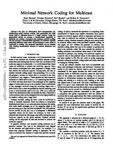
Fig. 1. A network with a source s with multi-resolution codes X1 , X2 , and X3 , and receivers r1 , r2 , r3 , r4 .

q(v)

c(e1 ,m1)

v C(u3)=Ø: q(u3)=0 q(u2) r

c(e2 ,m2)

v

Receiver: q(r) = minCut(r) C(v)

e1 e2

u2

c(e4 ,m4)

c(e3 ,m3) C(v)

e3

e4

u3

u

10

as 2 . The performance gain of this algorithm increases as the number of receivers increases and as the network grows in size, if appropriate criterion is used. Otherwise, na¨ıve interlayer coding may lead to an inappropriate choice of network code, which can be worse than intra-layer network coding. The rest of this paper is organized as follows. A network model and the network coding problem of multicast of multiresolution codes are established in Section II. The pushback algorithm is proposed in Section III, and proved in Section IV to guarantee decodability of the base layer. Simulation results are presented in Section V, while discussions on future work conclude the paper in Section VI. II. P ROBLEM S ETUP We consider the network coding problem for single-source multicast of multi-resolution codes, as illustrated by Figure 1. The single-source multicast network of interest is modeled by a directed acyclic graph G = (V, E), V being the set of nodes, and E the set of links. Each link is assumed to have unit capacity, while links with capacities greater than 1 are modeled with multiple parallel links. The subset R = {r1 , r2 , ...rn } ⊆ V is the set of receivers which wish to receive information from the source node s ∈ V . The source processes, X1 , X2 , ..., XL , constitute a multi-resolution code, where X1 is the base layer and the rest are the refinement layers. It is important to note that layer Xi without layers X1 , X2 , ..., Xi−1 is not useful for any i. For simplicity, we assume each layer is of unit rate. Therefore, given a link e ∈ E, we can transmit one layer (or equivalent coded data rate) on e at a time. The min-cut between s and a node v is denoted by minCut(v), and we assume that every node v knows its minCut(v). Note that there are efficient algorithms, such as Ford-Fulkerson algorithm, that can compute minCut(v). Our goal is to design a simple and distributed algorithm that provides a coding strategy to maximize the total rate achieved by all receivers with the reception of the base layer guaranteed to all receivers. By Min-Cut Max-Flow bound, each receiver ri can receive at most minCut(ri ) layers (X1 , X2 , .., XminCut(ri ) ). We present the pushback algorithm, and compare its performance against other existing algorithms and against the theoretical bound of Min-Cut Max-Flow. III. P USHBACK A LGORITHM The pushback algorithm is a distributed algorithm which allows both intra-layer and inter-layer linear network coding. It consists of two stages: pushback and code assignment. In the pushback stage, messages initiated by the receivers are pushed up to the source, allowing upstream nodes to

Fig. 2.

Pushback stage and code assignment stage at node v.

gather information on the demand of any receiver reachable from them. Messages are passed from nodes to their parents. Initially, each receiver ri ∈ R requests for layers X1 , X2 , ..., XminCut(ri ) to its upstream nodes, i.e., the receiver ri requests to receive at a rate equal to its min-cut. An intermediate node v ∈ V computes a message, which depends on the value of minCut(v) and the requests from its children. Node v then pushes this message to its parents, indicating the layers which the parent node should encode together. The code assignment stage is initiated by the source once pushback stage is completed. Random linear network codes [13] are generated in a top-down fashion according to the pushback messages. The source s generates codes according to the messages from its children: s encodes the requested layers together and transmits the encoded data to the corresponding child. Intermediate nodes then encode/decode the packets according to the messages determined during pushback. To describe the algorithm formally, we introduce some additional notations. For a node v, let P (v) be its set of parent nodes, and C(v) its children as shown in Figure 2. P (v) and C(v) are disjoint since the graph is acyclic. Let Evin = {(v1 , v2 ) ∈ E | v2 = v} be the set of incoming links, and Evout = {(v1 , v2 ) ∈ E | v1 = v} the set of outgoing links. A. Pushback Stage As shown in Figure 2, we denote the message received by node v from a child u ∈ C(v) as q(u), and the set of messages received by node v from its children as q(C(v)) = {q(u)|u ∈ C(v)}. A message q(u) means that u requests its parents to code across layers 1 to at most q(u). Once requests are received from all of its children, v computes its message q(v) and sends the same message q(v) to all of its parents. if v is a receiver then q(v) = minCut(v); end if v is an intermediate node then if C(v) = ∅ then q(v) = 0; end if C(v) 6= ∅ then q(v) = f (q(C(v)), minCut(v)); end end Algorithm 1: The pushback stage at node v.

3

s q(v1 )=2 v1

q(v2 )=1 v2

minCut(v1 )=1 minCut(v2 )=1 minCut(v3 )=2

q(v3 )=1 q(v3 )=1 v3

q(r1 )=2

q(r2 )=3 q(r1 )=2 q(r2 )=3

r1 minCut(r1)=2 Fig. 3.

q(r3 )=1 q(r2 )=3

r2 minCut(r2)=3

r3 minCut(r3)=1

An example of pushback stage with min-req criterion.

s q(v1 )=2 v1

q(v2 )=2 v2

q(v3 )=2

minCut(v1 )=1 minCut(v2 )=1 minCut(v3 )=2

q(v3 )=2 v3 q(r1 )=2

q(r1 )=2

r1 minCut(r1)=2

q(r2 )=3 q(r2 )=3

q(r3 )=1 q(r2 )=3

r2 minCut(r2)=3

r3 minCut(r3)=1

Fig. 4. An example of pushback stage with min-cut criterion. Highlighted are the messages different from that of min-req criterion (Figure 3).

The request q(v) is a function of q(C(v)) and minCut(v), i.e. q(v) = f (q(C(v)), minCut(v)). A pseudocode for the pushback stage at a node v ∈ V is shown in Algorithm 1. It is important to note the choice of f (·) is a key feature of the algorithm as it determines the performance. We present two different versions of f (·): min-req criterion and min-cut criterion, which we discuss next. 1) Min-req Criterion: The min-req criterion, as the name suggests, defines f (·) as follows: q(v) = f (q(C(v)), minCut(v)) ( 0 if q(u) = 0 for all u ∈ C(v), = qmin otherwise, where qmin = minq(u)6=0, u∈C(v) q(u) is the minimum nonzero q(u) from u ∈ C(v). This criterion may seem very pessimistic and na¨ıve, as the intermediate nodes serve only the minimum requested by their downstream receivers to ensure the decodability of the base layer. Nonetheless, as we shall see in Section V, the performance of this criterion is quite good. An example of pushback with min-req is shown in Figure 3. Receivers r1 , r2 , and r3 request their min-cut values 2, 3, and 1, respectively. The intermediate nodes v1 , v2 , and v3 request the minimum of all the requests received, which are 2, 1, and 1, respectively. 2) Min-cut Criterion: The min-cut criterion defines the function f (·) as follows: q(v) = f (q(C(v)), minCut(v)) ( qmin if minCut(v) ≤ qmin , = minCut(v) otherwise,

if v is the source s then foreach edge e = (v, u) ∈ Evout do v transmits c(e, q(u)); end end if v is an intermediate node then if P (v) = ∅ then v sets c(e, 0) for all e ∈ Evout ; end if P (v) 6= ∅ then v receives codes c(ei , mi ), ei ∈ Evin ; v determines m∗ , which is the maximum m such that X1 , X2 , ...Xm are decodable from c(ei , mi )’s; foreach child u ∈ C(v) do Let e = (v, u); if q(u) ≤ m∗ then v decodes layers X1 , X2 , ..., Xm∗ ; v transmits c(e, q(u)); end if q(u) > m∗ then Let mmax = maxmi ≤q(u) mi ; v transmits c(e, mmax ); end end end end if v is a receiver then v receives codes c(ei , mi ), ei ∈ Evin ; v decodes m∗ layers, which is the maximum m such that X1 , X2 , ...Xm are decodable from c(ei , mi )’s; end Algorithm 2: The code assignment stage at node v.

where qmin = minq(u)6=0, u∈C(v) q(u). Note if a node v receives minCut(v) number of linearly independent packets coded across layers 1 to minCut(v), it can decode layers X1 , X2 , ..., XminCut(v) and act as a secondary source with those layers. Thus, if there is at least one child u ∈ C(v) that requests fewer than minCut(v) layers, i.e. minCut(v) > qmin , node v sets its request q(v) to minCut(v). However, if all nodes request more than minCut(v) layers, node v does not have sufficient capacity to decode the layers requested by its children. Thus, it sets q(v) = qmin . An example of pushback with min-cut is shown in Figure 4. The network is identical to that of Figure 3. Again, the nodes r1 , r2 , r3 , and v1 request 2, 3, 1, and 2, respectively. However, node v2 requests 2, which is the minimum of all the requests it received, and node v3 requests minCut(v3 ) = 2. B. Code Assignment Stage This stage is initiated by the source after pushback is completed. As shown in Figure 2, c(e, m) denotes the random linear network code v transmits to its child u ∈ C(v), where e = (v, u), and m means that packets on e are coded across layers 1 to m. Note m may not equal to q(u), which we

4

n

n

s c(e1 ,2 ) e1

v1

c(e2 ,1) e2 v2

e3

c(e3 ,1)

minCut(v1 )=1 minCut(v2 )=1 minCut(v3 )=2

e6

M

n

e4 c(e4 ,1 )

v3 e8 c(e8 ,1) e9 e10 c(e10 ,1 ) c(e5 ,2 ) c(e ,1) c(e ,2 ) 7 6 c(e9 ,1 ) r2 r3 r1 minCut(r1)=2 minCut(r2)=3 minCut(r3)=1 Decodes 2 layers Decodes 2 layers Decodes 1 layer Fig. 5. An example of code assignment stage with min-req criterion. e5

e7

All non-zero elements are independently and randomly selected.

(a)

(b)

Fig. 7. Coding matrix M ; each row represents a code received, and columns represent the layers. The maximum number of non-zero columns in M , ck , can be equal to n (as shown in (a)), or less than n (as shown in (b)).

Generally the min-cut criterion achieves higher throughput than the min-req criterion. IV. A NALYSIS

s c(e1 ,2 ) e1

v1 e5 c(e5 ,2 )

e6 c(e7 ,2)

r1 minCut(r1)=2 Decodes 2 layers

c(e2 ,2) e 2 v2 e7

e8 c(e8 ,2) c(e6 ,2 )

e3 c(e3 ,2) e4 c(e4 ,2 ) e9 c(e9 ,2 )

r2 minCut(r2)=3 Decodes 2 layers

minCut(v1 )=1 minCut(v2 )=1 minCut(v3 )=2

v3 decodes layers 1 and 2 e10 c(e10 ,1 ) r3 minCut(r3)=1 Decodes 1 layer

Fig. 6. An example of code assignment stage with min-cut criterion. High– lighted are the messages different from the min-req criterion (Figure 5).

discuss in more detail in Section IV. Algorithm 2 presents a pseudocode for the code assignment stage at any node v ∈ V . Algorithm 2 considers source, intermediate, and receiver nodes separately. The source always exactly satisfies any requests from its children, while the receivers decode as many consecutive layers as they can. For an intermediate node v connected to the network (P (v) 6= ∅), v collects all the codes c(ei , mi ) from its parents and determines m∗ , the number of layers up to which v can decode. It is possible that v cannot decode any layer, leading to an m∗ equal to zero. For m∗ 6= 0, v can act as a secondary source for layers 1, 2, ..., m∗ by decoding these layers. In the case where q(u) ≤ m∗ , u ∈ C(v), v can satisfy u’s request exactly by encoding just the layers 1 to q(u). If q(u) > m∗ , v cannot decode the layers u requested; thus, cannot satisfy u’s request exactly. Therefore, v uses a best effort approach and delivers a packet coded across mmax layers, where mmax is the closest to q(u) node v can serve without violating u’s request, i.e. q(u) ≥ mmax . The code assignment stage requires that every node checks its decodability to determine m∗ . This process involves Gauss-Jordan elimination, which is computationally cheaper than matrix inversion required for decoding. Note that only a subset of the nodes need to perform (partial) decoding. Figures 5 and 6 illustrate the code assignment stage for the examples in Figures 3 and 4, respectively. Note that the algorithm for code assignment stays the same, whether we use min-req or min-cut criterion during the pushback stage; however, the resulting code assignments are different. Although the throughput achieved in this example network in Figures 5 and 6 are the same, this is usually not the case.

M

n

OF

P USHBACK A LGORITHM

In general, not all receivers can achieve their min-cuts through linear network coding. Nonetheless, we want to guarantee that no receiver is denied service, i.e. although some nodes may not receive up to the number of layers they requested, all should receive at least layer 1. In this section, we prove that the pushback algorithm guarantees decodability of the base layer, X1 , at all receivers. Two related lemmas are presented to prove Theorem 4.3. Lemma 4.1: Assume minCut(v) = n for a node v in G. In the pushback algorithm, if mi ≤ n for all c(ei , mi ), ei ∈ Evin , then v can decode at least layer 1 with high probability. In other words, if all received codes at v are combinations of at most n layers, v can decode at least layer 1. Proof: Recall that in the pushback algorithm, a code c(ei , mi ) represents coding across layers 1 to mi ; if the field size is large, with high probability, the first mi elements of this coding vector are non-zero, whereas the rest are zeros. Since minCut(v) = n, there exist n edge-disjoint paths from the source s to v, for all links are assumed to have unit capacity. Therefore, v receives from its incoming links at least n codes, each of which can be represented as a row coding vector of length n, since mi < n for all i. We pick the n codes corresponding to the edge-disjoint paths to obtain an n × n coding matrix. For the square coding matrix, we sort its rows according to the number of non-zero elements per row, obtaining the structure shown in Figure 7. We denote this sorted matrix by M , and the unique numbers of non-zero elements in its rows by c1 , c2 , ..., ck , in ascending order. Since the rows of M are generated along edge-disjoint paths using random linear network coding, the non-zero elements of M are independently and randomly selected. Next, we define upper-left corner submatrices M1 , M2 , ..., Mk as shown in Figure 8, where each submatrix Mi is of size ri × ci . More specifically, the rows of M with exactly c1 non-zero elements form a r1 × c1 submatrix M1 ; the rows of M with exactly c1 or c2 non-zero elements form the r2 × c2 c1 r1

c2

c3

M1 r2

Fig. 8.

M2

r3

M3

Upper-left corner submatrices M1 , M2 , and M3 .

5

v code c(e,m) q(v’) = q

Fig. 9.

v’ Node v and its child v′ .

submatrix M2 . Mk is of size rk × ck , where rk = n, and ck ≤ n. Note for any Mi of those submatrices, if rank(Mi ) = ci , node v can decode layers 1 to ci , i.e., the base layer is decodable. In other words, layer 1 is not decodable at node v only if rank(Mi ) < ci for all i. With these definitions, we assume layer 1 is not decodable at node v, and prove the lemma by contradiction. Specifically, we prove by induction that this assumption implies ri < ci for all i, leading to the contradiction rk < ck . For the base case, first consider M1 . If layer 1 is not decodable, rank(M1 ) < c1 . Recall that elements in M1 are independently and randomly selected [13]; if r1 ≥ c1 , with high probability, rank(M1 ) = c1 . Therefore, the above assumption implies r1 < c1 and rank(M1 ) = r1 . Next consider M2 . Under the assumption that layer 1 is not decodable, rank(M2 ) < c2 . Since rank(M1 ) = r1 and M2 includes rows of M1 , rank(M2 ) ≥ r1 . Rows r1 + 1, r1 + 2, ..., r2 are called the additional rows introduced in M2 . If there are more than c2 −r1 additional rows, M2 has full rank, i.e. rank(M2 ) = c2 , with high probability. Hence, the number of additional rows in M2 must be less than c2 − r1 , implying r2 < c2 . For the inductive step, consider Mi , 3 ≤ i ≤ k. Assume that rj < cj for all j < i. If layer 1 is not decodable, rank(Mi ) < ci . By similar arguments as above, rank(Mi−1 ) = ri−1 , and there must be less than ci − ri−1 additional rows introduced in Mi . Thus, ri < ci . By induction, the total number of rows rk = n in M is strictly less than ck ≤ n, which is a contradiction. We therefore conclude that node v can decode the base layer. In fact, v can decode at least c1 layers. Lemma 4.2: In the pushback algorithm, for each link e = (v, v ′ ), assume that node v ′ sends request q(v ′ ) = q to node v. Then, the code c(e, m) on link e is coded across at most q layers, i.e. m ≤ q (see Figure 9). Proof: First, we define the notion of levels. A node u is in level i if the longest path from s to u is i, as shown in Figure 10. Since the graph is acyclic, each node has a finite level number. We shall use induction on the levels to prove that this lemma holds for both min-req and min-cut criteria. For the base case, if v ′ is in level 1, it is directly connected to the source, and receives a code across exactly q layers on e s level 1

level 3

Fig. 10.

Level 1 and level 3 node in a network.

from s. For the inductive step, assume that all nodes in levels 1 to i, 1 ≤ i < k, get packets coded across layers 1 to at most their request. Assume v ′ is in level i+1 as in Figure 9. Let v ∈ P (v ′ ); therefore, v is in level j ≤ i. Let qmin be the smallest non-zero request at v, that is qmin = minq(u)6=0,u∈C(v) q(u). For the min-req criterion, v always sends request q(v) = qmin to its parents, and the codes v receives are linear combinations of at most qmin layers. Therefore, the code v sends to its children is coded across at most qmin layers, where q = q(v ′ ) ≥ qmin . In other words, the code received by v ′ is coded across at most q layers. For the min-cut criterion, if qmin > minCut(v), node v requests q(v) = qmin to its parents. By the same argument as that for the min-req criterion, v ′ receives packets coded across at most q layers. If qmin ≤ minCut(v), v requests q(v) = minCut(v). According to the code assignment stage, if v cannot satisfy request q exactly, it will send out a linear combination of the layers it can decode. Since v is in level j ≤ i, v receives codes across layers 1 to at most minCut(v). By Lemma 4.1, node v can decode at least the base layer. Thus, we conclude that node v is always able to generate a code for node v ′ such that it is coded across layers 1 to at most q. Theorem 4.3: In the pushback algorithm, every receiver can decode at least the base layer. Proof: The receiver with min-cut n receives linear combination of at most n layers by Lemma 4.2. From Lemma 4.1, the receiver, therefore, can decode at least the base layer. V. S IMULATIONS To evaluate the effectiveness of the pushback algorithm, we implemented it in Matlab, and compared the performance with both routing and intra-layered network coding schemes. Random networks were generated, with a fixed number of receivers randomly selected from the vertex set. We consider two metrics to evaluate the performance: % Happy Nodes = % Rate Achieved =

100 # of trials 100

X

# of receivers that achieve min-cut

all trials

P total all trials P

# of receivers rate achieved

total min-cut all trials

,

.

The % Happy Nodes metric is the average of the percentage of receivers that achieved their min-cut, i.e. receivers that received the service they requested. The % Rate Achieved metric gives a measure of what percentage of the total requested rate was delivered to the receivers over all trials. As an example, consider two possible cases where the (min-cut, achieved-rates) pairs are ([1, 1, 2], [1, 1, 1]) and ([2, 2, 3], [2, 2, 2]). In both cases, the demand of a single receiver is missed by one layer, but the corresponding fractions of rates achieved are 3/4 and 6/7 respectively. Using only the % Happy Nodes metric would tell us that 1/3 of the receivers did not received all requested layers. However, the % Rate Achieved metric provides a more accurate measure of how ‘unhappy’ the overall network is.

6

A. Algorithms for comparison 1) Point-to-point Routing Algorithm: the point-to-point routing algorithm considers each multicast as a set of unicasts. The source node s first multicasts the base layer X1 to all receivers. To determine the links used for layer X1 , s computes the shortest path to each of the receivers separately. Given the shortest paths to all receivers, s then takes the union of the paths and uses all the links in this union to transmit the base layer. Note the shortest path to receiver ri may not be disjoint with the shortest path to receiver rj . After transmitting layer Xi−1 , 2 ≤ i ≤ L, the source s uses the remaining network capacity to transmit the next refinement layer Xi to as many receivers as possible. First, s updates the min-cut to all receivers and identifies receivers that can receive Xi . Let R′ = {ri1 , ri2 , ...} be the set of receivers with updated min-cut greater than 1 and, therefore, can receive layer Xi . The source s then computes the shortest paths to receivers in R′ . The union of these paths is used to transmit the refinement layer. Node s repeats this process until no receiver can be reached or there are no more layers to transmit. 2) Steiner Tree Routing Algorithm: the Steiner tree routing algorithm computes the minimal-cost tree connecting the source s and all the receivers. We assume that each link is of unit cost. For the base layer X1 , s computes and transmits on the Steiner tree connecting to all receivers. For each new refinement layer Xi , s computes a new Steiner tree to receivers with updated min-cuts greater than zero. Node s repeats this process to transmit more refinement layers until no receiver can be reached or the layers are exhausted. It is important to note that Steiner tree routing algorithm is an optimal routing algorithm – it uses the fewest number of links to transmit each layer. Unlike the point-to-point algorithm, this algorithm may make routing decisions that is not optimal to any single receiver, i.e. the source may use a non-shortest path to communicate to a receiver, but it uses fewer links globally. However, this optimality comes with a cost: the problem of finding a Steiner tree is NP-complete. 3) Intra-layer Network Coding Algorithm: the intra-layer network coding algorithm uses linear coding on each layer separately. It iteratively solves the linear programming problem for linear network coding for layer Xi with receivers Ri = {r ∈ R | minCut(r) ≥ 1}, where i = 1 and R1 = R initially [14]. After solving the linear program for layer Xi , the algorithm increments i, updates the link capacities, and performs the next round of linear programming. References [8] and [9] are examples of this intra-layer coding approach. B. Implementation of Pushback Algorithm The pushback algorithm was implemented with two different message passing schedules. 1) Sequential Message Passing: for the pushback stage, each node in the network sends a request to its parents after request messages from all its children have been received. For the code assignment stage, each node sends a code to its children after receiving codes from all

its parents. This schedule corresponds to the algorithms explained in Section III. 2) Flooding: for the pushback stage, each node updates its request to its parents upon reception of a new message from its children. For the code assignment stage, each node sends a new code to its children after receiving a new message from any of its parent nodes. This allows an update mechanism that converges to the same solution as Sequential Message Passing. In fact, the convergence time depends on the diameter of the graph. Another important issue is the procedure to check decodability at each node. In general, Gauss-Jordan elimination on the coding matrix in field of size p, Fp , is necessary to determine which layers can be decoded at a node after the codes are assigned. However, this is not the case for 2-layer multiresolution codes. We define pattern of coding coefficients for a node with L incoming links as [a1 , a2 , ..., aL ], where ai represents the number of layers combined in the i-th incoming link for that node. If a node receives only the base layer on all incoming links, i.e. the pattern of coding coefficients is [1, 1, ..., 1], it can decode this single layer immediately. If at least one of the incoming links contains a combination of two layers, i.e. the pattern of coding coefficients is one the the following: [1, ..., 1, 2], [1, ..., 1, 2, 2], ..., [1, 2, ..., 2], [2, ..., 2], both layers can be decoded as well. In other words, if there are only two layers, the pattern of coding coefficients indicates decodability. We note that using the pattern of coding coefficients for decodability is equivalent to using Gauss-Jordan elimination with infinite field size. In more general cases with more than 2 layers, the pattern of coding coefficients is not sufficient to determine decodability. For example, a node with 4 incoming links of unit rate can have a min-cut of at most 4. Assume that a node with 4 incoming links has a min-cut of 3, and that this node is assigned a coding-coefficient pattern of [1, 1, 3, 3]. If all coding vectors are linearly independent, all layers are decodable. However, it is possible that the third and the fourth links, both combining three layers, are not from disjoint paths, i.e. they provide linearly dependent combinations. In such cases, Gauss-Jordan elimination is necessary to check that only the first layer is decodable. In subsequent sections, we present simulation results for 2 and 3-layer multi-resolution codes. However, our algorithm is not limited to 2 and 3-layers; it can be applied to general n-layer multi-resolution codes. C. Simulation results for 2-layer multi-resolution code The simulations for 2-layer multi-resolution code were carried out for random directed acyclic networks. We averaged 1000 trials for each data point on the curves plotted in this section. The networks were generated such that the min-cuts and the in-degrees of all nodes were less than or equal to 2. As mentioned in Section V-B, the patterns of coding coefficients are sufficient to check decodability for 2-layer multiresolution codes, and it is equivalent to using Gauss-Jordan elimination with an infinite field size. In Figure 11, we study

7

100

100

90 95

70

% of Happy Nodes

% Happy Nodes

80

60 50 PB min−cut p = 2m

40

m

PB min−req p = 2 PB min−cut p = ∞ PB min−req p = ∞

30 20 10 1

2

3

4

5

6

7

8

9

10

11

90

85

80

75

12

m

m (p = 2 )

Fig. 11.

70 3

Varying field size in a network with 5 receivers and 25 nodes.

pt2pt Steiner Layered PB min−req flooding PB min−cut flooding PB min−req sequential PB min−cut sequential 10 PB min−req p = 2 10 PB min−cut p = 2 4

5

6

7

8

9

7

8

9

No. of Receivers (|R|) 100

95

% Rate Achieved

the effect of field size in a network with 25 nodes and 5 receivers by performing Gauss-Jordan elimination at every node during the code generation stage with varying field size p. Figure 11 shows the average performance in terms of % Happy Nodes of our pushback algorithm with the mincut and min-req criteria against that of using the pattern of coding coefficients to check decodability. In essence, we are comparing the performance of our system using specific field sizes to that of an infinite field size. It is important to note that even for moderately small field sizes, such as p ≥ 28 , the pushback algorithm performs close to that of the system operating at an infinite field size. Simulation results also illustrate that the min-cut criterion performs considerably better than the min-req criterion for large field sizes, as shown in Figure 11. However, for small field sizes (p ≤ 23 ), the min-req criterion is slightly better. This is because the min-req criterion forwards the minimum of the requests received at any node. In the case of a 2-layer multicast, there will be more nodes requesting only the base layer in a network using the min-req criterion than that using the min-cut criterion. Thus, the network using the min-req criterion will have more links carrying only the base layer, which helps improve redundancy for the receivers. This allows several paths to carry the same information, ensuring the decodability of the first layer at the receivers. By comparison, the min-cut criterion tries to combine both layers at as many links as possible. When the field size is large, both layers are decodable with high probability; however, when the field size is small, the probability of generating linearly dependent codes is high. As a result, when p is small, this mixing can prevent decodability of both layers at a subset of receivers. In Figures 12 and 13, we compare the performance of the various schemes in terms of the two metrics % Happy Nodes and % Rate Achieved. We compare our pushback algorithm to that of Point-to-point Routing Algorithm (‘pt2pt’), Steiner Tree Routing Algorithm (‘Steiner’), and Intra-layer Network Coding Algorithm (‘Layered’). We also compare the two implementations of our algorithm (flooding and sequential message passing). The flooding approaches with an infinite field size are labeled ‘PB min-req flooding’ and ‘PB min-cut flooding’ for min-req and min-cut criteria, respectively. The

90

85

80

75 3

pt2pt Steiner Layered PB min−req flooding PB min−cut flooding PB min−req sequential PB min−cut sequential 10 PB min−cut p = 2 PB min−req p = 210 4

5

6

No. of Receivers (|R|)

Fig. 12.

Varying number of receivers in a network with 25 nodes.

sequential message passing approaches with an infinite field size are labeled ‘PB min-req sequential’ and ‘PB min-cut sequential’ for min-req and min-cut criteria, respectively. Finally, we include results when a moderate field size (p = 210 ) is used. These are labeled ‘PB min-req p = 210 ’ and ‘PB mincut p = 210 ’ for the min-req and min-cut criteria, respectively. Figure 12 shows the performance of the various schemes when we increase the number of receivers in the network. The pushback algorithm with min-cut criterion has the best performance overall. The flooding approach and the sequential message passing approach have the same performance, and furthermore, using a moderate field size of p = 210 yields results close to that of an infinite field size. This can be seen for both the min-cut and the min-req versions. Note that the performance of the various scheme follow a similar trend for both metrics % Happy Nodes and % Rate Achieved. In addition, Figure 12 illustrates that the gap between the min-cut version of our algorithm and ‘pt2pt’, ‘Steiner’ and ‘Layered’ increases with the number of receivers in the network. Note that the gap between the min-cut and the minreq criteria increases more slowly than the gap between the min-cut and the other schemes. Figure 13 compares the performance of the different schemes with fixed number of receivers and varying number of nodes in the network. Note our algorithm with the mincut criterion outperforms the intra-layer network coding and

8

100

100

98

95

96

90

% Happy Nodes

% Happy Nodes

94 92 90 88 86 84 82 80 10

pt2pt Steiner Layered PB min−req flooding PB min−cut flooding PB min−req sequential PB min−cut sequential 10 PB min−req p = 2 PB min−cut p = 210 15

20

25

85 80 75

pt2pt Steiner Layered

70 65

m

PB min−req p=2 60

30

35

40

45

50

55 3

m

PB min−cut p=2 4

5

6

7

8

9

10

11

12

m

No. Nodes (n)

m (p= 2 )

100

Fig. 14.

Varying field size in a network with 9 receivers 25 nodes.

98

% Rate Achieved

96 94 92 90 88 86 84 82 80 10

pt2pt Steiner Layered PB min−req flooding PB min−cut flooding PB min−req sequential PB min−cut sequential 10 PB min−cut p = 2 PB min−req p = 210 15

20

25

30

35

40

45

50

No. Nodes (n)

Fig. 13.

Varying number of nodes in a network with 3 receivers.

the routing schemes. In fact, the min-cut criterion consistently achieves close to 100% for both % Happy Nodes and % Rate Achieved while the second best scheme (‘Layered’) achieves at most 96% and 97% for the two metrics. Figure 13 shows that the performance of the min-cut criterion is very robust to the number of nodes in the network. In fact, the performance improves as more nodes are available. However, the min-req version degrades with the number of nodes. This is because, when using the min-req criterion, the requests from receivers with min-cut equal to one limits the rate of other receivers. When the network becomes large, this flooding of base layer requests has a more significant effect on the throughput as there are more resources wasted in delivering just the base layer. This indicates that the choice of network code can greatly impact the overall network performance, depending on its topology and demands. An inappropriate choice of network code can be detrimental, shown by the minreq criterion (‘PB min-req’); however, an intelligent choice of network code can improve the performance significantly, shown by the min-cut criterion (‘PB min-cut’). D. Simulation results for 3-layer multi-resolution code Similarly to the 2-layer case, for 3-layer multi-resolution codes, we generated random networks to evaluate the pushback algorithm. For each data point in the plots, we averaged 1000 trials. The min-cuts and the in-degrees of all nodes were less than or equal to 3. Recall that with 3 layers, the patterns of

coding coefficients are not sufficient for checking the decodability of incoming packets. Instead, Gauss-Jordan elimination is necessary at every node during the code generation stage. Figure 14 illustrates the effect of field size given a network of 25 nodes and 9 receivers. The pushback algorithm with the min-cut criterion (‘PB min-cut’) outperforms routing and intralayer coding schemes (‘Layered’) with a field size of p = 25 . Note, in terms of % Happy Nodes, ‘PB min-cut’ achieves roughly 92% when the field size is large enough, while the intra-layer coding scheme only achieves about 82%. Figure 14 also illustrates that intra-layer coding scheme still outperforms the routing schemes, even when optimal multicast routing is used for each layer (‘Steiner’). Our pushback algorithm achieves considerably higher gains by performing inter-layer in addition to intra-layer coding. As the number of receivers increases, more demands need to be satisfied simultaneously. It is therefore expected that the overall performance of multicast schemes will degrade with the number of receivers. This can be observed in Figures 15. Nonetheless, the performance gap between our two criteria of pushback (‘PB min-cut’ and ‘PB min-req’) remains approximately constant, while the performance gain over other schemes increases. This means that our algorithm is more robust to changes in the number of receivers than the other schemes, an important property for systems that aim to provide service to a large number of heterogeneous users. Figure 16 illustrates the performance of the different schemes when we increase the number of nodes in the network. As the number of nodes increases, there are more disjoint paths within the network for Steiner tree routing and intra-layer coding to use. Hence the performance of these schemes improves. The opposite behavior occurs for the pushback algorithm with the min-req criterion, i.e. the % Happy Nodes decreases with an increase in the number of nodes in the network. This result is similar to that of Figure 13 for 2-layer case. Note that as the number of nodes in the network increases, it becomes more likely that a small request by one receiver suppresses higher requests by many other receivers. Hence, pushback with the min-req criterion quickly deteriorates in terms of % Happy Nodes.

9

100 95

% Happy Nodes

90 85 80 75 70 65 60 55 3

pt2pt Steiner Layered PB min−req p=212 PB min−cut p=212 4

5

6

7

8

9

10

11

12

No. of Receivers (|R|) 100

% Rate Achieved

95

90

85

80

75 3

pt2pt Steiner Layered 12 PB min−req p=2 12 PB min−cut p=2 4

5

R EFERENCES

6

7

8

9

10

11

12

No. of Receivers (|R|)

Fig. 15. Varying number of receivers in a network with 25 nodes using field size of 212 . 100 95

% Happy Nodes

90 85 80 75 70

pt2pt Steiner Layered 10

65

PB min−req, p=2

10

PB min−cut, p=2 60 10

15

20

receivers increases and as the network grows in size as shown by numerical simulations. Possible future work includes the addition of a third complaint stage, in which receivers whose requests have not been satisfied pass another set of requests to their parents, signaling their desire for more. In generating new codes, parent nodes must take into account the new updated requests, while maintaining decodability at receivers which did not participate in the complaint stage. It is important to determine what the complaint messages should be, and to assess the improvements that can be achieved with such an additional stage. Another important extension is to apply this algorithm in wireless/dynamic multicast settings. The flooding approach (Section V) is applicable to such settings, as changes in the network can be handled by new messages to the neighboring nodes. An important extension is to study the performance and the convergence of this flooding approach in dynamic settings. Lastly, in the pushback algorithm, rate is the message sent by nodes to their parens, i.e. each node signals how many layers down-stream receivers can or want to receive. It may be possible to extend the message to include other constraints, such as power (decoding power), delay, and reliability.

25

30

35

40

45

50

No. of Nodes (n)

Fig. 16. Varying number of nodes in a network with 9 receivers using field size of 210 .

VI. C ONCLUSIONS

AND

F UTURE

WORK

A simple, distributed message passing algorithm, called the pushback algorithm, has been proposed to generate network codes for single source multicast of multi-resolution codes. With two stages, the pushback algorithm guarantees decodability of the base layer at all receivers. In terms of total rate achieved, this algorithm outperforms routing schemes as well as intra-layer coding schemes, even with small field sizes such as 210 . The performance gain increases as the number of

[1] A. Albanese, J. Bl¨omer, J. Edmonds, M. Luby, and M. Sudan, “Priority encoding transmission,” IEEE Transactions on Information Theory, vol. 42, no. 6, pp. 1737–1744, 1996. [2] N. Shacham, “Multipoint communication by hierarchically encoded data,” in Proceedings of INFOCOM ’92, 1992, pp. 2107–2114. [3] M. Effros, “Universal multiresolution source codes,” IEEE Transactions on Information Theory, vol. 47, no. 6, pp. 2113–2129, 2001. [4] R. Ahlswede, N. Cai, S.-Y. R. Li, and R. W. Yeung, “Network information flow,” IEEE Transactions on Information Theory, vol. 46, no. 4, pp. 1204–1216, July 2000. [5] R. K¨otter and M. M´edard, “An algebraic approach to network coding,” IEEE/ACM Transactions on Networking, vol. 11, no. 5, pp. 782–795, 2003. [6] D. Silva and F. R. Kschischang, “Rank-metric codes for priority encoding transmission with network coding,” in Proceedings of 10th Canadian Workshop on Information Theory (CWIT’07), June 2007. [7] J. M. Walsh and S. Weber, “A concatenated network coding scheme for multimedia transmission,” in Proceedings of 4th Workshop on Network Coding, Theory and Applications (NetCod’08), Jan 2008. [8] X. Wu, B. Ma, and N. Sarshar, “Rainbow network flow of multiple description codes,” IEEE Transactions on Information Theory, vol. 54, no. 10, pp. 4565–4574, 2008. [9] S. B. Niveditha Sundaram, Parameswaran Ramanathan, “Multirate media stream using network coding,” in Proceedings of 43rd Annual Allerton Conference on Communication, Control, and Computing, 2005. [10] J. Zhao, F. Yang, Q. Zhang, Z. Zhang, and F. Zhang, “Lion: Layered overlay multicast with network coding,” IEEE Transactions on Multimedia, vol. 8, no. 5, pp. 1021–1032, Oct. 2006. [11] C. Xu, Y. Xu, C. Zhan, R. Wu, and Q. Wang, “On network coding based multirate video streaming in directed networks,” in Proceedings of IEEE International Conference on Performance, Computing, and Communications, IPCCC‘07, April 2007. [12] S. Dumitrescu, M. Shao, and X. Wu, “Layered multicast with interlayer network coding,” in The 28th IEEE Conference on Computer Communications (INFOCOM’09), April 2009. [13] T. Ho, R. Koetter, M. M´edard, M. Effros, J. Shi, and D. Karger, “A random linear network coding approach to multicast,” IEEE Transactions on Information Theory, vol. 52, no. 10, pp. 4413–4430, October 2006. [14] D. S. Lun, N. Ratnakar, M. M´edard, R. Koetter, D. R. Karger, T. Ho, E. Ahmed, and F. Zhao, “Minimum-cost multicast over coded packet network,” IEEE Transactions on Information Theory, vol. 52, no. 6, pp. 2608–2623, June 2006.