ik. (j) of this new incoming traffic will flow over (i, k), and to first order, this will cause an increment delay on that link of. ϵÏm ik(j)Dik(tm i (j)Ïm ik(j)) where. Dik(tm.
1
Optimal Distributed Multicast Routing using Network Coding: Theory and Applications Yi Cui, Yuan Xue, Klara Nahrstedt Department of Computer Science, University of Illinois at Urbana-Champaign {yicui, xue, klara}@cs.uiuc.edu
Abstract— Multicast is an important communication paradigm, also a problem well known for its difficulty (NPcompleteness) to achieve certain optimization goals, such as minimum network delay. Recent advances in network coding[1], [2] has shed a new light onto this problem. In network coding, forwarding nodes can perform arbitrary operations on data received, other than forwarding or replicating, to enhance throughput of a multicast session. In this paper, we show that with the aid of network coding, the once intractable optimal multicast routing problem becomes tractable. In this problem, given a set of multicast sessions and their traffic demands, one tries to route the multicast traffic regarding various objectives, such as to minimize overall delay, or to maximize the battery life of each node. We further show that this problem can be solved in a distributed fashion: each node makes its own routing decisions based on periodic updating information from neighboring nodes. We prove that starting from any initial routing assignment, the proposed distributed routing algorithm is able to converge to the point where the value of the objective function is optimized. Our solution can be fit into a variety of networks to achieve different optimization goals. The examples in this paper include minimum delay routing in overlay multicast, and maximum lifetime routing in multi-hop wireless network.
I. I NTRODUCTION Optimal data routing in a network can be often understood as a multicommodity flow problem. Given a network and a set of commodities, i.e., a set of sourcedestination pairs, one tries to achieve certain optimization goal, such as minimum delay, maximum throughput, while maintaining certain fairness among all commodities. The constraints of such optimization problems are usually network link capacity and traffic demand of each commodity. Multicommodity flow problem has been well studied as a typical linear programming problem. Its distributed solutions have also been proposed[3][4]. However, when each commodity becomes a multicast session consisting of a source and several destination nodes, the same problem becomes intractable even in a centralized fashion. If the goal is to minimize network
delay, it becomes the Steiner tree problem, which is NPhard[5]. If the goal is to maximize achievable throughput, its difficulty is equivalent to packing Steiner trees, a problem even harder[6], [7], [8]. Recent advances on network coding has shed a new light onto this problem. Network coding generalizes traditional routing paradigm in which relaying nodes can only forward or replicate, by allowing them to perform arbitrary operation on information received to generate output. It is proved [1][2] that with network coding, the achievable throughput of a multicast session is the minimum of the maximum flow from the sender to any receiver. Given network coding’s amazing ability at improving throughput of existing network, we do not consider it the most wanted feature, since throughput is not the most urgent issue at the current moment. With the rapid advancement of optical fiber and ultraband technologies, the present (and ever growing) capacities of both wireline and wireless networks can easily satisfy the demands of current applications. What we consider the biggest advantage of network coding is the discovery that it makes the once intractable optimal multicast routing problem tractable. Furthermore, we show that this problem can be solved in an entirely distributed fashion. The problem is roughly defined as follows. Given a network, a set of multicast sessions, each with their own traffic demands, we try to route the multicast traffic regarding various objectives, such as to avoid congestion, minimize overall delay, or to maximize the battery life of each node in a wireless network. The rigorous definitions of these objective functions are given in Sec. III. With the aid of network coding, we are able to formulate the optimal multicast routing problem in the fashion of multicommodity flow (details in Sec. II). The major contribution of this work is an optimal distributed solution to the same problem. In this solution, each node makes its own routing decisions based on periodic updating information from neighboring nodes. More importantly, starting from any initial routing assignment,
2
it should finally converge to the optimal point, such as minimum network delay. Our solution inherits the same design philosophy of Gallager’s algorithm[3], but is significantly different from it, since we try to achieve optimal routing in the setting of multicast communication with network coding. Although our solution is general enough to fit into a variety of networks to achieve different optimization goals, we consider it more suitable to be employed in a new generation of application-level networks, such as overlay network, multi-hop wireless network, etc. In these networks, each node is flexible enough to be configured to perform various operations. In contrast, traditional Internet is already too rigid to even turn on its multicast switch, not to mention adding new functionalities such as network coding. Moreover, multicast plays an essential role in the most popular applications supported by these new networks, such as overlay multicast[9], P2P content distribution, wireless sensor network, etc. They often has a system goal such as lifetime maximization in sensor network, i.e., to maximize the duration that all sensor nodes are up until one of them has its battery drained. Such a goal of “system optimization” is radically different to “user optimization”, which is the goal of most current networking algorithms. In Internet, each node attempts to send each packet over a route that minimizes that packet’s delay with no regard to other packet’s delays. If the same analogy is applied to sensor network routing, each node would attempt to minimize the amount of energy it spends on each packet transmitted, which deviates from the system optimization goal of maximum lifetime. We believe our solution is well suited to achieve the goal of “system optimization” in the above mentioned network and application settings. Due to space constraint, we only report theoretical result of our work. The rest of this paper is organized as follows. We briefly go over the concept of network coding and present our network model in Sec. II. In Sec. III, we first discuss necessary and sufficient conditions to achieve optimal routing in the general network model, then illustrate two particular examples: minimum-delay routing in overlay network and maximum-lifetime routing in multihop wireless network. Sec. IV presents our distributed routing algorithm and proves that it is able to converge to the point where the value of the objective function is optimized. Sec. V discusses some practical issues. Finally, Sec. VI concludes the paper.
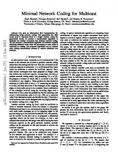
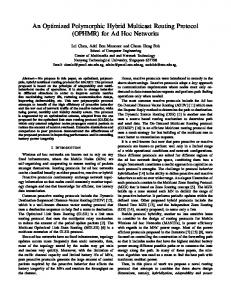
II. P RELIMINARIES A. Network Coding: The Concept An example to illustrate the concept of network coding is shown in Fig. 1. Consider a directed network in which each link has identical capacity. We have a multicast session where S is the sender, R1 and R2 are receivers. a and b represent two independent information flows originating from the sender S . As shown in Fig. 1 (b), node 3 transmits the coded flow a ⊕ b along the “bottleneck” link (3, 4) to node 4, which in turn forwards the coded flow to receivers r1 and r2 , which can recover {a, b} from {a, a ⊕ b} and {b, a ⊕ b}. On the other hand, without network coding (Fig. 1 (a)), receivers r1 and r2 can only receive one of the two flows. It is proved by Ahlswede et al.[1] that with network coding, the achievable throughput of a multicast session can be acquired by running max-flow algorithm from the source to each individual receiver, then choosing the minimal result. Koetter et al.[2] prove the same result using algebraic approach. Li et al.[10] further shows that the above result can be obtained by running linear coding. Chou et al.[11] are the first to propose a practical network coding solution. s a
s a
b
1
2
b
1
2 a
3
3
a
b
a
a⊕b r2
(a) Throughput without Network Coding Fig. 1.
b
a⊕b
4 r1
b
r1
4
a⊕b r2
(b) Throughput with Network Coding
The Effects of Network Coding
B. Network Model We consider a n-node network, where the nodes are represented as N = {1, 2, . . . , n}. Let L be the set of links, denoted as L = {(i, k) | a link goes from i to k}. Each link (i, k) is associated with a capacity Cik . There are a set of multicast sessions M. For each session m ∈ M, it has a sender S(m), and a set of receivers R(m). Let rim (j) ≥ 0 be the traffic of session m, in bits/s, generating at node i and destined for node j (data sink). rim (j) > 0 only if node i = S(m), and j ∈ R(m), i.e., if node i is the sender of session m, and node j is one of
3
the receivers of m. We also define node flow tm i (j) to be the total traffic of session m at node i destined for node m j . tm i (j) includes both ri (j) and the traffic from other nodes that is routed through i to destination j . Finally, m φm ik (j) is the fraction of the node flow ti (j) routed over link (i, k). It is always true that φm /L ik (j) = 0 if (i, k) ∈ (no traffic can be routed through non-existent link), or i = j (traffic that has reached its destination is not sent back into the network). Also, node i must route its entire node flow tm i (j) through all links, i.e., X
φm ik (j) = 1, ∀i, j ∈ N , ∀m ∈ M
(1)
k∈N
Now we express the relation of above notations as follows: X m m tm tm i (j) = ri (j) + l (j)φli (j), ∀i, j ∈ N , ∀m ∈ M l∈N
(2) Eq. (2) expresses flow conservation: for a given multicast session s, the traffic into a node for a given destination is equal to the traffic out of it for the same destination. Lemma 1 Given the input set r and routing variable set φ, the set of equations (2) has a unique solution for t. Each element ti (j) is nonnegative and continuously differentiable as a function of r and φ. For each session s, we define the amount of traffic on link (i, k) as the union of all flows through it. m m fik = max tm i (j)φik (j), ∀(i, k) ∈ L j
(3)
According to Alhswede et al.[1], for a given input set r = {rim (j) | i, j ∈ N , m ∈ M}, if there exists a routing solution φ = {φm ik (j) | i, j, k ∈ N , m ∈ M} that is feasible, i.e., fik =
X
m fik ≤ Cik , ∀(i, k) ∈ L
(4)
m∈M
then the achievable throughput by network coding in m each multicast session m is minj∈R(m) rS(m) (j). Furthermore, any feasible solution is schedulable by a network coding assignment. Now we can formalize our “system optimization” goal according to the following format. For example, if the delay on each link (i, k) is a function of traffic on it, Dik (fik ), and our goal is to minimize the overall network delay, it can be formalized into the following
optimization problem. D:
minimize
D=
X
Dik (fik )
(i,k)∈L
subject to (1), (2)(flow constraint) (3)(union of flow constraint) (4)(capacity constraint)
III. O PTIMALITY C ONDITIONS FOR D ISTRIBUTED M ULTICAST ROUTING In this section, we analyze the optimality conditions for distributed multicast routing. We show that when the system delay D is minimized, within each session m, each node i, for a given receiver j , the partial derivative of D to the routing variable φm ik (j) (marginal delay on link (i, k)) is the same for all links (i, k) originating from node i. An analogy is that within an electrical network where each wire has different resistance, certain currents flow from the sender node to the receiver node. By Dirichlet principle, the potentials taken within the electrical network minimize the total energy dissipation. And when it happens, the potentials (partial derivative of energy dissipation to currents) of all wires sharing the same positive end are the same. Sec. III-A goes through the formal analysis to reach the above result. Note that although we use delay as an example objective, the same conclusion holds for any type of objective function. In Sec. III-B and III-C, we show that with necessary adjustment to the network model and objective function, we can derive the same optimality conditions for multicast routing in a wide spectrum of problem settings. Our examples include minimum delay routing in overlay multicast, and maximum lifetime routing in multi-hop wireless network. A. General Model We calculate the partial derivatives of the delay D with respect to the inputs r and the routing variables φ. We first consider ∂D/∂rim (j). Assume a small increment ² in the input rim (j). For each adjacent node k , an increment ²φm ik (j) of this new incoming traffic will flow over (i, k), and to first order, this will cause an increment delay on that link of 0 m m ²φm ik (j)Dik (ti (j)φik (j))
where 0 m Dik (tm i (j)φik (j)) =
m dfik dDik (fik ) dfik · m· m dfik dfik d(tm i (j)φik (j))
4 0 (tm (j)φm (j)) can be calculated as follows. A Dik i ik commonly used link delay function is defined by Kleinrock[12] as follows. fik Dik (fik ) = (5) (Cik − fik )
This function assumes that queueing delays are the only noneligible source of delay in a network, and each link traffic can be modelled as Poisson message arrivals with independent exponentially distributed lengths. In fact, we do not need to know what Dik (fik ) is, as long as this function is increasing and convex in fik . In practice, we can also choose to directly measure Dik and its derivative, which we will discuss in Sec. V-A. m = 1. According to According to Eq. (4), dfik /dfik Eq. (3), m 1/n if tm i (j)φik (j) and n − 1 m dfik other flows on link(i, k) = m m are the maximum d(ti (j)φik (j)) 0 otherwise (6) If node k is not the destination node, then the increment ²φm ik (j) of extra traffic at node k will cause the same incremental delay onward as an increment ²φm ik (j) of new input traffic at node k . To first order this m incremental delay will be ²φm ik (j)∂D/∂rk (j). Summing over all adjacent nodes k , then, we find that, h X ∂D i ∂D m 0 m m φ (j) D (t (j)φ (j)) + = i ik ik ik ∂rim (j) ∂rkm (j) k∈N X m φm (7) = ik (j)δik (j) k∈N 0 (tm (j)φm (j)) + ∂D Here, = Dik i ik ∂rkm (j) is called the marginal delay of link (i, k) with respect to receiver j . (7) asserts that the marginal delay of a node is the convex sum of the marginal delays of its outgoing links with respect to the same destination. By the definition of φ, we can see that ∂D/∂rjm (j) = 0, since φm jk (j) = 0, i.e., no traffic of receiver j needs to be routed anymore once it arrives to the destination. m Next consider ∂D/∂φm ik (j). An increment ² in φik (j) m causes an increment ²ti (j) in the portion of tm i (j) flowing on link (i, k). If k 6= j , this causes an addition ²tm i (j) to the traffic at k destined for j . Thus for (i, k) ∈ L, i 6= j , h ∂D ∂D i m 0 m m = t (j) D (t (j)φ (j)) + i ik i ik ∂φm ∂rkm (j) ik (j) m m = ti (j)δik (j) (8) m (j) δik
To summarize above discussions, we have the following theorems.
Theorem 1: Let a network have inputs r and routing variables φ, and let each marginal delay dDik (fik )/dfik be continuous in fik , (i, k) ∈ L. Then the set of equations (7), i 6= j , has a unique (and correct) set of solutions for ∂D/∂rim (j). Furthermore, (16) is valid and both ∂D/∂rim (j) and ∂D/∂φm ik (j) for i 6= j , (i, k) ∈ L are continuous in r and φ. Theorem 2: Assume that Dik is convex and continuously differentiable for fik . let ψ be the set of φ, the necessary condition for φ to minimize D over ψ is ½ m ∂D = minl ∂D/∂φm il (j) if φik > 0 (9) m m ≥ minl ∂D/∂φil (j) if φik = 0 ∂φm ik (j) and the sufficient condition for φ to minimize D over ψ is m δik (j) ≥
∂D , ∀i 6= j, (i, k) ∈ L, ∀m ∈ M ∂rim (j)
(10)
The necessary condition (9) in Theorem 2 states that within session m, at node i, for a given receiver j , all links (i, k) that have any portion of flow tm i (j) routed through (φm (j) > 0 ) must achieve the same ik minimum marginal delay with respect to j , and that this minimum marginal delay must be less than or equal to the same marginal delays of the links with no flow routed (φm ik (j) = 0). The sufficient condition (10) states that within session m, at node i, for a given receiver j , the marginal delay of all links (i, k) with respect to j must be greater than or equal to the marginal delay of node i. B. Minimum Delay Routing in Overlay Multicast In the setting of overlay network, we need to redefine the link set L since each link (i, k) ∈ L is actually a unicast route going through a set of physical links. Let Z be the set of physical links encompassed by the overlay network L, we define function nz (i, k). nz (i, k) = 1 if link (i, k) goes through the physical link z ∈ Z , and 0 otherwise. The capacity constraint (4) should be rephrased as X X m fz = nz (i, k) fik ≤ Cz , ∀z ∈ Z (11) (i,k)∈L
m∈M
Also the delay of link (i, k) is the aggregate delay of all physical links it goes through. Therefore, X Dik (fik ) = nz (i, k)Dz (fz ) (12) z∈Z
5
Then our goal is formalized into the following problem1 . X O: minimize D = Dik (fik ) (i,k)∈L
subject to (1), (2)(flow constraint) (3)(union of flow constraint) (11)(capacity constraint)
Now let us first derive partial derivative of delay D to an input variable rim (j). X X ∂D ∂Dz (fz ) = nz (k, l) m (13) m ∂ri (j) ∂ri (j)
Corollary 1: Assume Dik is convex and continuously differentiable for fik , let ψ be the set of φ, the necessary condition for φ to minimize D over ψ is ½ m ∂D = minl ∂D/∂φm il (j) if φik > 0 (16) m ≥ minl ∂D/∂φm ∂φm il (j) if φik = 0 ik (j) and the sufficient condition for φ to minimize D over ψ is ∂Dik (fik ) ∂D ∂D + m ≥ m m ∂ri (j) ∂rk (j) ∂ri (j) ∀i 6= j, (i, k) ∈ L, ∀m ∈ M
(17)
(k,l)∈L z∈Z
C. Maximum lifetime Routing in Multihop Wireless Netwhere work ∂Dz (fz ) = (14) m ∂ri (j) In multi-hop wireless network such as sensor network, m m (j)) X dfkl d(tm (j)φ dDz (fz ) data is sent through wireless link, which consumes k kl nz (k, l) m m m limited battery energy of both sender node and receiver dfz d(tk (j)φkl (j)) dri (j) (k,l)∈L node. Energy-efficient routing thus becomes an imporHere, dDz (fz )/dfz is the marginal delay of the phys- tant issue. Our goal here is to maximize the lifetime of m /d(tm (j)φm (j)) can be ical link z , the definition of dfkl the network, i.e., the duration in which all nodes are up k kl found at (6), and until one of them is drained of energy. m m Y X We define Ei the energy reserve at node i. Let pri d(tk (j)φkl (j)) m m φnp (j) (J/bit) be the power consumption at node i, when it φkl (j) = drim (j) all paths P from i to k (n,p)∈P receives one unit of data, and ptik (J/bit) be the power (15) consumption when one unit of data is sent from i over Eq. (15) means that if there is a small increment ² link (i, k). Based on the first order radio model, we have on the input rim (j), the corresponding increment on link the following. m m (k, l) will be ² · d(tm k (j)φkl (j))/dri (j). Summarizing over Eq. (14) and (15), we find out that pri = a (18) Eq. (13) can be simplified into the following recursive t θ pik = a + b · (dik ) (19) form: h ∂D (f ) X ∂D ∂D i ik ik m Here, a is a distance-independent constant that repreφ (j) = + ik ∂rim (j) ∂rim (j) ∂rkm (j) sents the energy consumption to run the transmitter or k∈N receiver circuitry, and b is the coefficient of the distancewhich is similar to (7). dependent term that represents the transmit amplifier. dik Following the same way, we derive the partial derivais the distance from node i to k . The exponent θ is m tive of D to routing variable φik (j) as follows. determined from field measurements, which is typically h ∂D (f ) i ∂D ∂D ik ik a constant between 2 and 4. The power consumption = tm i (j) m (j) + ∂r m (j) ∂φm (j) ∂r ratio (J/s) of node i is i ik k X£ ¤ It can be easily verified that within the overlay pi = fik · ptik + fki · pr , ∀i ∈ N (20) network setting, Theorem 1 still holds. From the k∈N definition of Dik in Eq. (12), we can see that if the physical link delay Dz (fz ) is convex and continuously Now it is clear that the lifetime of node i is differentiable, Dik is also convex and continuously Ei differentiable. Therefore, we are able to reach the (21) Ti = pi following conclusion, which is similar to Theorem 2. 1 In definitions (11) and (12), we can see that the physical link z can be either unidirectional or bidirectional.
Our target is to maximize the minimum lifetime of all nodes, i.e., the duration that all nodes within the network are up. Associating Ti with a utility Ui , this goal can be
6
formalized as to maximize the aggregate utility of all nodes as follows. X X T 1−γ i ,γ → ∞ U: maximize U = Ui = 1−γ i∈N
i∈N
subject to (1), (2)(flow constraint) (3)(union of flow constraint) (4)(capacity constraint) (20), (21)(power constraint)
Here γ can be made an arbitrarily large number to infinitely approximate the optimal value. We first consider ∂U/∂rim (j), the marginal utility on node i with respect to receiver j . Assume that there is a small increment ² on the input traffic rim (j). Then ²φm ik (j) from this new incoming traffic will flow over wireless link (i, k). This will cause an increment power consumption on node i, t ²φm ik (j)pik
m dfik m d(tm i (j)φik (j))
in order to send out the incremented traffic. The defim /d(tm (j)φm (j)) can be found at Eq. (6). nition of dfik i ik And the consequent utility change of node i is 0 t ²φm ik (j)Ui (pi )pik
m dfik m d(ti (j)φm ik (j))
Similarly, on the receiver side, the utility change of node k is m dfik 0 r ²φm (j)U (p )p ik k k k m d(tm i (j)φik (j)) If node k is not the destination node, then the increment ²φm ik (j) of extra traffic at node k will cause the same utility change onward as a result of the increment ²φm ik (j) of input traffic at node k . To first order this utility change will be ²φm ik (j)∂U/∂rk (j). Summing over all adjacent nodes k , then, we find that, h ∂U X ∂U m = φ (j) + ik ∂rim (j) ∂rkm (j) k∈N i df m (ptik Ui0 (pi ) + prk Uk0 (pk )) m ik m d(ti (j)φik (j)) h X ∂U i 0 m m (22) = φm (j) U (t (j)φ (j)) + ik ik i ik ∂rkm (j) k∈N
0 (tm (j)φm (j)) = (pt U 0 (p ) + pr U 0 (p )) · where Uik i k k k ik i i ik m dfik is called the marginal utility on link (i, k), m m d(ti (j)φik (j)) ∂U m m 0 and Uik (ti (j)φik (j)) + ∂rm (j) is called the marginal k
utility of link (i, k) with respect to receiver j . (7) asserts that the marginal utility of a node is the convex sum of the marginal utilities of its outgoing links
with respect to the same receiver. By the definition of φ, we can see that ∂U/∂rjm (j) = 0, since φm jk (j) = 0, i.e., no traffic of receiver j needs to be routed anymore once it arrives to the destination. Next we consider ∂U/∂φm ik (j). An increment ² in m φik (j) causes an increment ²tm i (j) in the portion of tm (j) flowing on link (i, k) . If k 6= j , this causes an i addition ²tm (j) to the traffic at k destined for j . Thus i for (i, k) ∈ L, i 6= j , h ∂U i ∂U 0 m m m (t (j)φ (j)) + (j) U = t (23) i ik ik i ∂φm ∂rkm (j) ik (j) We are able to prove the following corollaries similar to Theorem 1 and 2. Corollary 2: Let a wireless network have inputs r and routing variables φ, and let each marginal utility Ui0 (pi ) be continuous in pi , i ∈ N . Then the set of equations (22), i 6= j , has a unique (and correct) set of solutions for ∂U/∂rim (j). Furthermore, (23) is valid and both ∂U/∂rim (j) and ∂U/∂φm ik (j) for i 6= j , (i, k) ∈ L are continuous in r and φ. Corollary 3: Assume that Ui is concave and continuously differentiable for pi . let ψ be the set of φ, the necessary condition for φ to maximize U over ψ is ½ m ∂U = maxl ∂U/∂φm il (j) if φik > 0 (24) m ≤ maxl ∂U/∂φm ∂φm il (j) if φik = 0 ik (j) and the sufficient condition for φ to maximize U over ψ is ∂U ∂U ≤ m m ∂rk (j) ∂ri (j) ∀i 6= j, (i, k) ∈ L, ∀m ∈ M
0 m Uik (tm i (j)φik (j)) +
(25)
Note that since U is decreasing and concave in fik while D is increasing and convex in fik , the optimality conditions in Corollary 3 are exactly opposite to the ones in Theorem 2. Also note that by (21) and the definition of U , we can see that U is concave as long as Eq. (20) is convex in fik . Therefore, as long as it is a convex function of fik , the power consumption model does not need to follow the definition in Eq. (19) and (18). IV. D ISTRIBUTED ROUTING A LGORITHM By understanding the optimality conditions (general model discussed in Sec. III-A) to multicast routing, the design philosophy of our routing scheme should now be clear. The algorithm works in an iterative fashion. In each iteration, for each session m, each node i and
7
a given receiver j , i must incrementally increase the fraction of traffic on link (i, k) (by increasing φm ik (j)) m whose marginal delay δik (j) is small, and do the reverse for those links whose marginal delay is big, until the marginal delays of all links carrying traffic are equal. When this condition is met for all nodes regarding all receivers within all sessions, the entire system reaches the optimal point. Therefore, for each session m, each node i, each iteration involves two steps: (1) the calculation of marginal 0 (tm (j)φm (j)) for each outgoing link (i, k), delay Dik i ik and each of its downstream neighbors k ’s marginal delay ∂D/∂rkm (j); (2) the adjustment of routing variables m 0 m φm ik (j) based on the values of Dik (ti (j)φik (j)) and ∂D/∂rkm (j). We will elaborate them in details as follows. Sec. IV-A introduces how the calculation and update 0 (tm (j)φm (j)) and ∂D/∂r m (j) of marginal delays Dik i ik k are executed. Sec. IV-B discusses how to maintain loopfree routing. Sec. IV-C formally presents the algorithm, whose optimal property is analyzed in Sec. IV-D. Finally, in Sec. IV-E and IV-F, we discuss how the algorithm should be adjusted in the setting of minimumdelay routing in overlay network and maximum-lifetime routing in wireless network. A. Calculation of Marginal Delays We first see how each node i calculates its marginal delay ∂D/∂rim (j), with respect to receiver j . In order to do so, based on Eq. (7), i needs to know δik (j) = 0 (tm (j)φm (j)) + ∂D/∂r m (j), the marginal delays of Dik i ik k all its outgoing links regarding receiver j . In Sec. III-A, 0 (tm (j)φm (j)), we have discussed how to calculate Dik i ik and ∂D/∂rkm (j) is the marginal delay of i’s downstream neighbor k . Now it is clear that ∂D/∂ri (j) should be calculated in a recursive way. Starting from receiver, ∂D/∂rjm (j) = 0 based on definition. j then sends the values of ∂D/∂rjm (j) to its upstream neighbor, say k . Upon receiving the updates, node k can calcu0 (tm (j)φm (j)) as described above, then acquire lates Dik i ik m ∂D/∂rk (j). Then, k repeats the same procedure to its upstream neighbor, until node i is reached.
is free of deadlock if and only if such a partial ordering is maintained, i.e., the routing variable set φ is loop free. In order to achieve loop-free routing, for each node i, m (j) of with respect to receiver j , we introduce a set Bi,φ m blocked nodes k for which φik (j) = 0 and the algorithm m is not permitted to increase φm ik (j) from 0. k ∈ Bi,φ (j) if one of the following conditions is met. 1) (i, k) ∈ / L, i.e., k is not the neighbor of i. 2) φm (j) = 0 and ∂D/∂rim (j) ≤ ∂D/∂rkm (j), i.e., ik the marginal delay of k is already greater than or equal to the marginal delay of i. 3) φm ik (j) = 0 and ∃(l, p) ∈ L such that (a) l = k or l is downstream to k with respect to receiver j ; (b) m m φm lp (j) > 0, and ∂D/∂rl (j) ≤ ∂D/∂rp (j), i.e., (l, p) is an improper link. An example illustrating improper link is shown in Fig. 2. The solid line indicates that there is traffic on this link, and the dotted line indicates otherwise. Here node 4 is a receiver of session m. The partial ordering of their marginal delays are 1 → 2 → 3 → 4, which the traffic from node 3 to 1 is against. Node 2, if unaware of the existence of such an improper link downstream, might make a loop by moving some of its outgoing traffic to node 3. To prevent this case from happening, node 3 only needs to raise a flag when updating its marginal delay to its upstream nodes 2 and 3. Upon receiving such a notification, nodes 2 and 3 can include node 3 into their blocking sets. m
∂ D / ∂ r3(4) = 4 2 p loo
1 m
improper link 3
loop
m
∂ D / ∂ r3(4) = 3
∂ D / ∂ r3(4) = 5 4 m
∂ D / ∂ r4(4) = 0
Fig. 2.
Illustration of Improper Link
C. Algorithm
B. Loop-free Routing From the above calculation, we can see that among all nodes carrying traffic of session m, their marginal delays follow a partial ordering. Each receiver j has the lowest marginal delay, which is 0. Its upstream neighbors have higher marginal delays, whose own upstream neighbors have even higher marginal delays. Therefore, the recursive procedure of node marginal delay calculation
Now we are ready to formalize our algorithm. We use to represent the routing variable set at the iteration k . ∆φ(k) is the changes made to φ(k) during the iteration k . Apparently, φ(k+1) = φ(k) + ∆φ(k) . Also for node i, m m T • φm i (j) = (φi1 (j), . . . , φin (j)) is the vector of its routing variable regarding receiver j and session m. m m T • ∆φi (j) = (∆φm i1 (j), . . . , ∆φin (j)) is the vector m of changes to φi (j). φ(k)
8 (k) should not turn φm (j)(k) to negative. The ∆φm il (j) il amount of reduction is also inversely proportional to tm i (j), since the change in link traffic is related to m (j)(k) tm (j). When tm (j) is small, ∆φm (j)(k) can ∆φ At iteration k , node i operates according to the following i i il il be changed by a large amount without greatly affecting steps. 1) For each session m, calculate link marginal delay the marginal delays. Finally, the change depends on the 0 (tm (j)φm (j)) for each of its outgoing links stepsize α. As shown later in Theorem 3, convergence Dik i ik (i, k), get updates of marginal delays ∂D/∂rkm (j) can be guaranteed if α is small enough. As α increases, from each of its downstream neighbors k , then cal- the speed of convergence increases but the danger of no convergence also increases. m (j) = D 0 (tm (j)φm (j)) + ∂D/∂r m (j). culate δik ik i ik k We can implement Mim (j)(k) differently to further 2) Calculate its own marginal delay ∂D/∂rim (j) acFor example, Bertsekas et cording to Eq. (7), and send it to all its upstream improve convergence speed. m (j)(k) as a diagonal matrix al.[4] choose to set M i neighbors. where the element at the lth row and lth column is the m (k) 3) Calculate φi (j) by solving the problem 2 second derivative of delay D to routing variable φm il (j), m (j) t 2 D/(∂φm (j))2 . m T m i i.e., ∂ · (26) minimize δi (j) ∆φi (j) + il 2α (k) T m (k) m (k) (∆φm i (j) ) Mi (j) ∆φi (j) D. Analysis •
m (j), . . . , δ m (j))T is the vector of δim (j) = (δi1 in marginal delays of all i’s neighbors.
(k) (k) subject to φm + ∆φm ≥ 0, i (j) i (j) The following lemma shows some of the properties X m (k) m (k) ∆φil (j) = 0, ∆φil (j) = 0, of our algorithm. l∈N m ∀l ∈ Bi,φ (k) (j)
where α > 0 is some positive stepsize, and matrix Mim (j)(k) is some symmetric matrix which m is P positivemdefinite on the subspace {∆φi (j) | l∈N ∆φil (j) = 0}. 4) Adjust routing variables (k+1) (k) (k) φm = φm + ∆φm i (j) i (j) i (j)
∀i ∈ N − {j}, ∀m ∈ M
Note that in problem (26), Mim (j)(k) can be any positive definite matrix, and any solution ∆φm i (j) to this problem will allocate more traffic on the link with the minimum marginal delay, and decrease traffic on other links. If we implement Mim (j)(k) as the identity matrix, the solution to ∆φm (j)(k) boils down to
Lemma 2: (a) If φ(k) is loop-free, then φ(k+1) is loop-free. (b) If φ(k) is loop-free and ∆φ(k) = 0 solves problem defined in step (3) of the algorithm, then φ(k) is optimal. (c) If φ(k) is optimal, then φ(k+1) is also optimal. (d) If ∆φ(k) 6= 0 for some i for which tm i (j) > 0, then there exists a positive scalar ηk such that D(φ(k) + η∆φ(k) ) < D(φ(k) ), ∀η ∈ (0, ηk ]
The following theorem shows the main convergence result.
Theorem 3: Let the initial routing φ(0) be loop-free and satisfy D(φ(0) ) ≤ D0 where D0 is some scalar. (k) Assume also that there exist two positive scalars λ, Λ ∆φm il (j) such that for each session m, each node i, and each m 0 if l ∈ Bi,φ(k) (j) receiver j , the sequences of matrices {Mim (j)(k) } satisfy − min{φm (j)(k) , il the following two conditions. m m = α(δil (j)−δmin (j)) m (j) } if δilm (j) 6= δmin m (a) The absolute value of each element of Mim (j)(k) t (j) P i m m (k) m if δil (j) = δmin (j) is bounded above by Λ. m m δip (j)6=δmin (j) ∆φip (j) (b) There holds m (j) = min where δmin p∈B / m (k) (j) δip (j). i,φ λ|vi |2 ≤ viT Mim (j)(k) vi This algorithm increase the fraction of traffic on the link with the minimum marginal delay, and reduces the for all v such that P m i l∈B / (j) vil = 0. i,φ(k) fraction of other links. The amount of reduction on link Then there exists a positive scalar α (depending on (k) m (i, l), given by ∆φm il (j) , is proportional to δil (j) − D , λ, and Λ) such that for all α ∈ (0, α] and k = 0 m δmin (j), the difference of marginal delays between (i, l) 2 2 itself and the link with the minimum marginal delay. In fact, since ∂ 2 D/(∂φm il (j)) is difficult to compute, this element (k) ≤ φm (j)(k) , i.e., is usually set to be its upper bound. (j) It is further restricted that ∆φm il il
9
0, 1, . . ., the sequence {φ(k) } generated by the algorithm satisfies D(φ(k+1) ) ≤ D(φ(k) ) lim D(φ(k+1) ) = min D(φ)
k→∞
φ∈ψ
Furthermore, every limit point of {φ(k) } is an optimal solution to problem defined in step (3) of the algorithm. E. Distributed Algorithm for Minimum-Delay Routing in Overlay Network From the optimality conditions (16) and (17) derived in Sec. III-B, we see that the algorithm presented in this section can be directly applied into the setting of overlay network. The only exception is that an overlay link (i, k) is a unicast route containing several physical links. Hence its delay (marginal delay) is the aggregate delay (marginal delay) of all these links. In order to calculate the marginal delay of (i, k), it is impractical, if not at all impossible, to calculate the marginal delays of all physical links on its route, then add them up. Instead, we can treat the delay function Dik as a black box and monitor the change of its output (end-to-end delay of overlay link (i, k)) reacting to the change of its input (rim (j)), then estimate its derivative (marginal delay ∂Dik /∂rim (j)). Such a technique is called perturbation analysis[13], which we will briefly mention in Sec. V-A. F. Distributed Algorithm for Maximum-Lifetime Routing in Wireless Network The algorithm for the general model can be applied into the setting of wireless network with the following changes. First, the calculation of link marginal mutility dfik 0 (tm (j)φm (j)) = (pt U 0 (p )+pr U 0 (p )) Uik m i ik ik i i k k k d(tm i (j)φik (j)) requires cooperation of both sender i and receiver k , since sending data over the wireless link (i, k) requires power consumption of both nodes. Node i can calcum /d(tm (j)φm (j)) based on Eq. (6). i is also late dfkl kl k responsible to calculate the term ptik Ui0 (pi ). Ui0 (pi ) can be derived based on the definition of U , if the energy reserve Ei and power consumption ratio pi are known. ptik can be calculated based on Eq. (19), if constants a, b, θ, and node distance dik are known beforehand. Node k is responsible to calculate the term prk Uk0 (pk ). Uk0 (ck ) can be calculated the same way as Ui0 (ci ). prk can be calculated based on Eq. (18). After calculation, k can send the value of prk Uk0 (pk ) to node i, which in turn 0 (tm (j)φm (j)). acquires Uik i ik
Second, by the optimality conditions (16) and (17) derived in Sec. III-B, and the fact that utility function U is decreasing and concave in fik , the algorithm should do the following. In each iteration, for each session m, each node i and a given receiver j , i must incrementally increase the fraction of traffic on link (i, k) whose marginal utility is great, and do the reverse for those links whose marginal utility is small, until the marginal utilities of all links carrying traffic are equal. Consequently, in the formal algorithm presented in Sec. IV-C, problem (26) should be redefined to: tm i (j) · (27) 2α (k) T m (k) m (k) (∆φm i (j) ) Mi (j) ∆φi (j)
maximize δim (j)T ∆φm i (j) −
subject to the same constraints. m (j), . . . , δ m (j))T is a vector where Here, δim (j) = (δi1 in m 0 m m δil (j) = Uil (ti (j)φm (j)) + ∂U/∂r il l (j), the marginal utility of link (i, l) in session m, with respect to receiver j . V. P RACTICAL I SSUES A. Measurements of Marginal Delay and Marginal Utility In the real minimum-delay routing environment, we cannot assume the delay function of a link to be exactly the same as what is defined in Eq. (5). In the setting of overlay network, the end host may not even know the capacity of some physical link its unicast route goes through. Furthermore, the overhead of calculating marginal delays of all physical links and aggregate them to acquire the marginal delay of an overlay link, is unacceptable, if such an operation is not at all impossible to execute. In [13], a procedure is presented for estimating online marginal packet delays through links with respect to link flows without making the standard assumptions (exponentially distributed packet lengths, Poisson arrival processes). This procedure is based on a technique known as perturbation analysis. No knowledge of network parameters (arrival rates, link capacities) is required. The same technique can be employed in both physical and overlay network environment. Similarly, in maximum-lifetime wireless routing environment, we can adopt the same approach. During the 0 (tm (j)φm (j)), node calculation of marginal utility Uik i ik i or k can estimate its power consumption ratio by directly measuring the amount of data sent and the corresponding energy dissipation during the most recent period, then derive the marginal utility based on Eq. (21) and the definition of U , both of which are predefined
10
independent of power consumption models of wireless nodes. B. Messaging Overhead In each iteration of our algorithm, the destination node of each link needs to update the marginal delay or marginal utility of this link to the source node. Therefore, a total of |L| messages need to be sent, |L| being the number of links inside the network. In case there are more than one multicast sessions, the number of messages required can stay unchanged if each node aggregates its marginal delays or marginal utilities regarding all sessions into a single message. Such messaging overhead can be further saved if we piggyback these messages into data/acknowledgement packets. C. Interference of Wireless Transmission It is well known that the achievable rates in multi-hop wireless network are not only constrained the capacities of wireless links, but also location-dependent contention and spatial reuse[14], [15]. Given the fact that deriving the optimal achievable rates is NP-hard, [15] gave an approximation algorithm, which is guaranteed to return a packet scheduling solution which is within 67% of the optimal solution. In our case, we can choose to run this scheduling algorithm, then reset the capacity Cik of each wireless link (i, k) to its maximal achievable rate. In this way, we guarantee that our routing solution is always schedulable at the price of suboptimal bandwidth utilization. As we have argued in the introduction, maximizing throughput is not the most urgent issue, given the current asymmetric situation of bandwidth supply and application demand in wireless network. Rather, we consider the battery energy on wireless node as the most precious resource, hence the lifetime of the entire network, which our algorithm tries to optimize. VI. C ONCLUSION This paper presents a general solution for optimal multicast routing. We show that with the aid of network coding, the once intractable optimal multicast routing problem becomes tractable. We further show that this problem can be solved in an entirely distributed fashion by presenting a distributed routing algorithm, which is proved to converge to the point where the value of the objective function is optimized. Our solution can be fit into a variety of networks to achieve different optimization goals, such as minimum delay routing in overlay multicast, and maximum lifetime routing in multi-hop wireless network.
VII. A PPENDIX A: P ROOF OF L EMMA 1 Proof: Without loss of generality, let us consider the commodity j in session m. We restate Eq. (2) as X m m tm tm i (j) = ri (j)+ l (j)φli (j), ∀i ∈ N , ∀m ∈ M l∈N −{j}
(28) since φm (j) = 0 . Summing both sides over i , we have lj X tm rim (j) (29) j (j) = i∈N
The physical meaning of (29) is obvious: in a session m, the amount of commodity arrived at node j equals the total amount generated from each of its sources. For the pure purpose of proof, we temporarily define φm ji (j) = m m ri (j)/tj (j) and substitute it into (28), we have X m tm tm (30) i (j) = l (j)φli (j), i ∈ N , m ∈ M l∈N
Any solution to (30) and (29) satisfies (28). Let ˆ m (j) be the n × n matrix with elements φm (j). Φ li ˆ m (j) is stochastic, since each element φm (j) ≥ 0, and Φ li Pn m i=1 φli (j) = 1 (1 ≤ i ≤ n,m ∈ M). Consequently, (30) is the formula for steady-state probabilities in a Markov chain. ˆ m (j) is irreducible, then (30) has a unique soluIf Φ ˆ m (j) irreducible, there has to tion. In order to make Φ exist a path between any pair i and k , i.e., φm il (j) > m m 0, φlm (j) > 0, . . . , φpk (j) > 0. To prove this, we only need to show that there exists a path from node j to any other node, and a path from any other node to j . For a node i, if ri (j) > 0, then there is a path from i to j . Otherwise, the traffic generated from i will not arrive at j , contradicting (29). Also by the temporary definition of m m φm ji (j) = ri (j)/tj (j), there is a path from j to i too. In m conclusion, if ri (j) > 0(i ∈ N − {j}, m ∈ M), then ˆ m (j) is irreducible, hence 30 has a unique solution, Φ where tm i (j) > 0(i ∈ N − {j}, m ∈ M). ˆ m (j), If we remove the j th column and j th row of Φ we acquire a (n − 1) × (n − 1) matrix Φm (j). If we define two row vectors as: m m m tm (j) = (tm 1 (j), . . . , tj−1 (j), tj+1 (j), . . . , tn (j)) m m r m (j) = (r1m (j), . . . , rj−1 (j), rj+1 (j), . . . , rnm (j))
then we can restate (28) into the following vector form: tm (j)(I − Φm (j)) = r m (j)
Since this equation has a unique solution if r m (j) > 0, I − Φm (j) must have an inverse. Therefore, tm (j) = r m (j)(I − Φm (j))−1
(31)
11
Since tm (j) is positive when r m (j) is positive, tm (j) is nonnegative when r m (j) is nonnegative. Now we differentiate tm (j) as a function of r m (j). Differentiating (31), we get the continuous function of Φm (j), ∂tm i (j) = [(I − Φm (j))−1 ]li ∂rlm (j)
(32)
tm i (j)
X
=
l∈N −{j}
∂tm i (j) m r (j) ∂rlm (j) l
∂tm l (j) φm li (j) ∂φm kp (j) m ∂tl (j) m φli (j) ∂φm kp (j)
+
tm k (j)
m ∇ · Dm (j) = (∂D/∂r1m (j), . . . , ∂D/∂rj−1 (j), m ∂D/∂rj+1 (j), . . . , ∂D/∂rnm (j))T
(33)
then we can rewrite (7) into the following vector form:
Now we differentiate tm (j) as a function of Φm (j). Differentiating (28) with φm kp (j), we get P m ∂ti (j) l∈N −{j} = P m ∂φkp (j) l∈N −{j}
Proof: Without loss of generality, let us consider j in session m. Let bm i (j) = P them commodity 0 m m k∈N φik (j)Dik (ri (j)φik (j)). We define two column vectors as: m m m T bm (j) = (bm 1 (j), . . . , bj−1 (j), bj+1 (j), . . . , bn (j))
Using (32) in (31), we can express the solution to (28) as
VIII. A PPENDIX B: P ROOF OF T HEOREM 1
∇ · Dm (j) = bm (j) + Φm (j)(∇ · Dm (j))
We saw in the proof of Lemma 1 that I − Φm has if i = p a unique inverse. Thus the unique solution to (36), otherwisecontinuous in Φ(j), is given by
(34) If we fix k and p, and introduce two variables αim (j) and βim (j) defined as ∂tm i (j) m (j) ∂φkp ½ m tk (j) if i = p βim (j) = 0 otherwise
αim (j) =
∇ · Dm (j) = (I − Φm (j))−1 bm (j) P m 0 m m Substituting k∈N φik (j)Dik (ti (j)φik (j)) back to the above equation, we have ∂D ∂rim (j)
X
αim (j)φm li (j), i ∈ N
l∈N −{j}
which has the same set of equations as (28), with αim (j) m corresponding to tm i (j), and βi (j) corresponding to m m ri (j). Also since βi (j) ≥ 0, we can repeat the same m derivation for tm i (j) and ri (j) and reach the same conclusion as in (32) and (33): ∂αim (j) ∂tm (j) = im = [(I − Φm (j))−1 ]li m ∂βl (j) ∂rl (j) αim (j) =
=
X ∂αm (j) ∂αim (j) m m i β (j) = β (j) ∂βlm (j) l ∂βpm (j) p
X ∂tm (j) X 0 m m l φm lp (j)Dlp (tl (j)φlp (j)) ∂rim (j)
p∈N ∂tm l (j) 0 D (tm (j)φm (37) φm (j) lp (j)) lp ∂rim (j) lp l (l,p)∈L
l∈N
=
(34) becomes αim (j) = βim (j) +
(36)
X
Finally, differentiating D with φm ik (j) using (3)), we have ∂D ∂φm ik (j)
=
X
0 m m Dlp (tm l (j)φlp (j))φlp (j)
(l,p)∈L 0 m m +Dik (tm i (j)φik (j))ti (j)
∂tm l (j) ∂φm ik (j)
Also from the proof of Lemma 1, we have ∂D ∂φm ik (j)
= tm i (j)
X
0 m m Dlp (tm l (j)φlp (j))φlp (j)
(l,p)∈L m 0 m +ti (j)Dik (tm i (j)φik (j))
∂tm l (j) ∂rkm (j)
l∈N
m
∂ti (j) Substituting ∂φ and tm m k (j) back to the above kp (j) equation, we have the solution, continuous in φm (j), as ∂tm ∂tm (j) i (j) = im tm (j) (35) m ∂φkp (j) ∂rp (j) k
By (37), we have h ∂D i ∂D m 0 m m = t (j) + D (t (j)φ (j)) i ik i ik ∂φm ∂rkm (j) ik (j)
which is the same as (16). Now we can conclude that (16) is continuous in φ(j) given the continuity of ti (j) . and ∂r∂D i (j)
12
A PPENDIX C: P ROOF OF T HEOREM 2 Proof: First we show that (9) is a necessary condition to minimize D by assuming that φ does not satisfy (9). This means that there exists a session m, and nodes i,j ,k , and p such that φik (j) > 0,
∂D(φ) ∂D(φ) > ∂φik (j) ∂φip (j)
(38) (39)
(i,k)∈L
Since each link delay Dik is a convex function of the link flow, D(λ) is convex in λ, and hence dD(λ) ¯¯ ≤ D(φ∗ ) − D(φ) ¯ dλ λ=0
Since φ∗ is arbitrary, proving that dD(λ)/dλ ≥ 0 at λ = 0 will complete the proof. From (39) to (38), X dDik (fik ) dD(λ) ¯¯ ∗ (fik − fik ) = ¯ dλ λ=0 dfik
(40)
(i,k)∈L
We now show that X dDik (fik ) X ∂D(φ) m∗ fik ≥ rkm (j) m dfik ∂rk (j)
(i,k)∈L
(j,k)∈L
i,j∈N
(i,k)∈L
X
m∗ tm∗ i (j)φik (j)
i,j,k∈N
Since these derivatives are continuous, a sufficiently small decrease in φm ik (j) and corresponding increase in φip (j) will decrease D, contradicting the fact that φ does not minimize D. Next we show that (10) is a sufficient condition to minimize D. Suppose that φ satisfies (10) and has node flows t and link flows f . Let φ∗ be any other set of routing variables with node flows t∗ and link flows f ∗ . Define ∗ fik (λ) = (1 − λ)fik + λfik X Dik (fik (λ)) D(λ) =
Further summing both sides of above equation over i, we have X X dDik (fik ) ∂D(φ) m∗ fik tm∗ ≥ − (43) i (j) dfik ∂rim (j)
(41)
∂D(φ) ∂rkm (j)
Substituting (2) into (43), we get (41). Note that if we replace φ∗ with φ in (42), (42) becomes an equality from the equation for ∂D/∂rim (j) in (7). For the same reason, if we replace φ∗ with φ in (43), (43) becomes X dDik (fik ) X ∂D(φ) m (44) fik = rkm (j) m dfik ∂rk (j) j,k
(i,k)∈L
Substituting (44) and (41) into (40), and summing over m, we see that dD(λ)/dλ ≥ 0 at λ = 0, which completes the proof. A PPENDIX D: P ROOF OF L EMMA 2 Proof: (a) Assume that φ(k+1) is not loop-free so that there exists a sequence of links forming a directed cycle along which φ(k+1) is positive. Also there must (k) ) ∂D(φ(k) ) exist a link (p, q) for which ∂D(φ ∂rm (j) ≤ ∂rm (j) . From p
q
m m (k) > 0 the definition of Bi,φ (k) (j) we must have φpq (j) and hence (p, q) is an improper link. Now move backwards around the cycle to the first link (i, l) for (k) = 0. Such a link must exist since φ(k) which φm il (j) is loop-free. Since node l is upstream of node p and m link (p, q) is improper, we have l ∈ Bi,φ (k) (j)) which m (k+1) contradicts the hypothesis φil (j) > 0.
(b) If ∆φ(k) = 0 solves problem (26), then we must m have δim (j)T ∆φm i (j) ≥ 0 for each node i and ∆φ (j) satisfying the constraints of (26). X m (k) m ∆φm ∆φm i (j) ≥ −φi (j) , il (j) = 0, ∀l ∈ Bi,φ(k) (j) l∈N
m m (k) and using By writing ∆φm i (j) = φi (j) − φi (j) (7), (16) we have X ∂D(φ) X ∂D(φ) ∗ 0 m m∗ m∗ Dik (ti (j)φik (j))φik (j) ≥ m − φ (j) m (k) ∂ri (j) ∂rkm (j) ik δim (j)T (φm i (j) − φi (j) ) k∈N k∈N X X (k) (42) = δilm (j)φm δilm (j)φm il (j) − il (j) ∗ Multiplying both sides of (42) by t (j), summing over l∈N l∈N X j , and recalling (6) and (3), we have ∂D = δilm (j)φm ≥0 il (j) − ∂rim (j) X dDik (fik ) X l∈N ∂D(φ) m∗ fik ≥ tm∗ − i (j) m dfik ∂rim (j) / Bi,φ By considering φm (k) (j), we j∈N k∈N il (j) = 1 for each l ∈ obtain X ∂D(φ) m∗ ∂D tm∗ m i (j)φik (j) ≤ δilm (j), ∀l ∈ / Bi,φ (k) (j) ∂rkm (j) ∂rim (j) j,k∈N
Note from (10) that
13
From (7) and (16) we have ∂D m m (k) = δilm (j), ∀l ∈ / Bi,φ >0 (k) (j), φil (j) ∂rim (j)
Since Dil0 > 0 for all (i, l) ∈ L it follows from (7), (16) and the relation above that there are not improper m links, and using the definition of Bi,φ (k) (j) we obtain ∂D = min δilm (j) l∈N ∂rim (j)
which is the same as (10), the sufficient condition for optimality of φ(k) . (c) If φ(k) is optimal then from the necessary condition for optimality (9) we have that for all node i with tm i (j) > 0 ∂D = min δ m (j) ∂rim (j) p∈N ip It follows using a reverse argument to the one in (k) = 0 if tm (j) > 0. Since changing (b) that ∆φm i i (j) only routing variables of nodes i for which tm i (j) = 0 does not affect the flow through each link we have D(φ(k) ) = D(φ(k+1) ) and φ(k+1) is optimal.
Using (46), we are able to prove that λ D(φ(k+1) ) − D(φ(k) ) ≤ ( + U |N |4 ) · α|N |3 X (k) 2 m (k+1) (k) 2 (tm − φm i (j) ) kφi (j) i (j) k i,j∈N
∀i, j ∈ N , m ∈ M (k)
00 (f (k) where U = max(i,l)∈L,φ∈ψ {Dik il ) | D(φ ) ≤ λ D0 }. Take α ∈ (0, α], α < |N |7 U we have X (k) 2 D(φ(k+1) ) − D(φ(k) ) ≤ −p (tm i (j) ) · (k+1) kφm i (j)
−
i,j m (k) 2 φi (j) k , ∀i, j
∈ N,m ∈ M
Thus, the sequence {D(φ(k) )}∞ k=1 is nonincreasing. Since Dik is bounded from below by 0, we obtain (45).
R EFERENCES
[1] R. Ahlswede, N. Cai, S.R. Li, and R.W. Yeung, “Network information flow,” IEEE Tran. Information Theory, vol. 46, 2000. [2] R. Koetter and M. Medard, “An algebraic approach to network coding,” IEEE Tran. Networking, vol. 11, 2003. [3] R. Gallager, “A minimum delay routing algorithm using m m (k) (d) If ti (j) > 0, then Mi (j) is positive definite distributed computation,” IEEE Tran. Commun., vol. 25, 1977. (k) 6= [4] D. Bertsekas, E. Gafni, and R. Gallager, “Second derivative on the appropriate subspace. If in addition ∆φm (j) i algorithms for minimum delay distributed routing in networks,” 0, then the second term in (26) is positive. Since the IEEE Tran. Commun., vol. 32, 1984. m T m (k) minimum in (26) is non-positive, δi (j) ∆φi (j) < [5] M. Garey and D. Johnson, Computers and Intractability: A 0. By (16), we obtain that Guide to the Theory of NP-Completeness, 1979. [6] M. Thimm, “On the approximability of the steiner tree prob³ ∂D ´T (k) lem,” in Mathematical Foundations of Computer Science. 2001, ∆φm