Sep 6, 2016 - that best integrates the joint process. ... and social platforms, such as Facebook and Twit- ter. ... monly seen social and technological networks.
Network Composition from Multi-layer Data Kristina Lerman1 , Shang-Hua Teng2 , and Xiaoran Yan3
arXiv:1609.01641v1 [cs.SI] 6 Sep 2016
1
Information Sciences Institute, University of Southern California 2 Computer Science, University of Southern California 3 Network Science Institute, Indiana University
Abstract
technological systems [30, 7, 15]. On top of these network structures, different dynamical processes unIt is common for people to access multiple social net- fold [8, 18, 19]. Our ability to model and predict works, for example, using phone, email, and social dynamic network phenomena has led to new applicamedia. Together, the multi-layer social interactions tions ranging from ranking web pages to maximizing form a “integrated social network.” How can we social influence and controlling epidemics [31, 11, 23]. extend well developed knowledge about single-layer Traditionally, most research has focused on the networks, including vertex centrality and community simple graph representation where all verticies and structure, to such heterogeneous structures? In this edges are of a single type. More recently, there has paper, we approach these challenges by proposing a been great interest in going beyond such a homogeprincipled framework of network composition based neous model to investigate networks that are capable on a unified dynamical process. Mathematically, we of capturing multiple types of connections. Extenconsider the following abstract problem: Given multisive efforts towards such heterogeneous models came layer network data, (G1 , . . . , Gl ) over a vertex set V from both social [34, 35] and computational disciand additional parameters for intra and inter-layer plines [25, 1], as the simple graph abstraction are dynamics, construct a (single) weighted network G often too crude a description of reality. For examthat best integrates the joint process. We use transple, it is very common for people to have interactions formations of dynamics to unify heterogeneous layers across multiple social networks, including neighbors, under a common dynamics. For inter-layer compocoworkers, and also online interactions through email sitions, we will consider several cases as the interand social platforms, such as Facebook and Twitlayer dynamics plays different roles in various social ter. Each of these networks underlies a different type or technological networks. Empirically, we provide of social interactions. Because of the different oriexamples to highlight the usefulness of this framegins and motivations, many names have been given work for network analysis and network design. to such heterogeneous models including but not limited to multiplex network, multi- relational networks, and networks of networks. For a comprehensive re1 Introduction view see [24]. In this paper, we adopt their terminology and use the general model of multi-layer netAs a powerful representation for many complex sysworks, with multiplex network being a special case tems, networks model entities and their interactions when inter-layer structures are absent. as vertices and edges. Studies of network structures, Structure and dynamics of multi-layer networks including those of vertex centrality and community structure have lead to fundamental insights into the have been explored in both theoretical graphs and organization and function of social, biological and real world data [4, 10, 12, 20, 16], with several re1
searchers generalizing community structure and centrality measures to multiple edge types [29, 28, 22, 6, 32, 33]. However, it remains an open research question as how to build a multi-layer network in the first place. Such networks are often constructed simply by stacking or projecting layers into a single network. When inter-layer edges are explicitly modeled, they usually appear as tunable parameters, despite the fact that general theoretical framework allows much richer representations [24]. One challenge for modeling inter-layer structures is that they are empirically difficult to measure in most cases [16, 17]. In this paper, instead of proposing multi-layer generalizations of network measures, we approach the problem by constructing a single composed network which integrates the multi-layer data. We propose a two-stage framework for multi-layer network composition based on a unified dynamical process, as illustrated by Figure 1. Specifically, the first stage address the layer heterogeneity through layer transformations. In Section 3, we discuss how to transform the layers into homogeneous Markov processes using the framework of the parameterized Laplacian [19]. In Section 4, we will discuss the second stage, which consists of several ways of combining layers in commonly seen social and technological networks. They include how to construct multiplex networks as well as multi-layer structures with observed inter-layer dynamics. In the multi-layer case, we choose to model a vertex’s inter-layer transitions, i.e., its participation in the different network layers, as another Markov process. Therefore, we can treat the combined layers of interlinked dynamical processes as a joint Markov process itself. We will prove that under this view a unique composition of a multi-layer network exists. In practice, however, it is difficult to fully observe inter-layer transitions. Hence, we will also consider the problem of network composition with partial information, for example, knowing only the stationary distribution of a inter-layer Markov process. Together, these dynamical process based transformations and compositions capture the heterogeneous structure while leaving a unified underlying topology. As a result, we can directly apply existing network algorithms of vertex centrality and community detection to the correctly composed joint structure. Some
Layer transformation
Inter-layer composition
Figure 1: A two-stage framework for multi-layer composition
of the applications of multi-layer formalism to realworld data are discussed in Section 5.
2
Preliminaries
In this section, we introduce some basic notations for multi-layer networks and dynamical processes. Single-layer data: A standard network is represented by weighted directed graph G = (V, E, A), where V = {1, ..., n} and for u, v ∈ V , auv ≥ 0 assigns an affinity weight to edge (u, v) ∈ E. We follow the convention that auv = 0 if and only if (u, v) 6∈ E. G may have self-loops, and edges in G are assumed to be directed. In other words, the weighted adjacency matrix A can be asymmetric and can have none-zero Pnentries on the diagonal. For u ∈ V , let = v=1 au,v denote dout u Pn the out-degree of vertex u. Similarly, let din u = v=1 av,u denote the in-degree of vertex u. In this paper, we use DA (or D when the context is clear) to denote the diagonal matrix whose entries are out-degrees. Multi-layer data: We consider vertex-aligned multilayer networks [24]. We usually use l to denote number of layers, and use Gi = (V, E i , Ai ) to denote the network at ith layer. For clarity, we will use superscripts i, j, r for the layers and subscripts u, v, w for vertices. Note that the vertex set V is the same across the layers. Figure 2 is a toy example of a threelayer network, consisting of (hypothetical) phone contacts, email exchanges and Facebook friendships of four users. In the figure, users appear in multiple layers, connected by a dashed line. 2
In this paper we take a dynamical view of the network structure. The simplest dynamical process on graphs G is the discrete time unbiased random walk (URW), represented by the transition matrix M . For their connections we have the following lemma:
Lemma 2 Suppose M is a detailed-balanced transition matrix with stationary π. Let Π be the diagonal matrix defined by π. Then, for all α > 0, α · M Π is symmetric. Namely, AM = {α · M Π} contains symmetric adjacency matrices if and only if M is detailed-balanced.
Lemma 1 For every directed network G = (V, E, A), there is a unique transition matrix, MA = Therefore, for undirected graphs, there is only one −1 ADA , that captures the URW Markov process on G. degree of freedom to specify the underlying network Conversely, given a transition matrix M , there is in for a given detailed-balanced transition matrix, which fact an infinite family of adjacency matrices whose can be interpreted as the global scaling factor. random walk Markov process is consistent with M : AM = {M Γ : Γ is a positive diagonal matrix.}
3
In other words, every directed network uniquely defines a random walk process. However, given a transition matrix M , there remains n degrees of freedom to specify the underlying network. Intuitively, they are vertex scaling factors bacause each random walk distribution remains the same as along as the whole column is multiplied together. We will use this fact in some of our construction. Recall that an n-dimensional probability vector π is the stationary distribution of M if M π = π. The Markov process defined by M is detailed-balanced if for all u, v ∈ V , πu muv = πv mvu . It is well known that [3]:
In [19], Ghosh et al. argued that perceived network structure is a result of the interplay between the network topology and the dynamical process on top of it. We believe this interplay is even more pronounced in multilayer networks, with each layer represents a different type of connection. It is essential to account for the different intra-layer dynamics before the composition. Taking Figure 2 for example, if we want to trace a message in the combined network, one should take into account the different propagating patterns in each layer. We might weigh the edges in the phone
ap bp p
c
Phone
ae ce
be de
cf
Email
bf
af df
Layer Transformation
Facebook
Figure 2: A toy example of multi-layer social network in horizontal perspective 3
layer much heavier if it is a business message. Similarly, each user may also has its own habits in terms of how often they check their email and Facebook accounts. In Section 2, we showed the mathematical mapping from the adjacency matrices to the transition matrices representing simple URWs. The parametrized Laplacian operator introduced in [19] can model a richer family of dynamical processes. As a conservative operator, it has a dominate eigenvalue 0, and models continuous time random random walks or consensus processes with various biases and delays at vertices. In this paper, we shall focus on the random walk formulation:
To reach homogeneity across the layers, we need to transform each input layer to equivalent graphs with URWs as the unifying dynamics. Using the two graph transformations under the parametrized Laplacian framework, we have Theorem 1 For a directed network G = (V, E, A), the dynamics L = (D 0 − BA)(D 0 T )−1 is equivalent to a URW on another transformed graph.
Proof The first transformation under the parametrized Laplacian framework is the bias transformation, which is already defined in the parentheses of Equation (1). A biased random walk from vertex u to v with transition probability (1) L = (D 0 − BA)(D 0 T )−1 . Pvu ∝ bv avu is equivalent to an unbiased random walk on a reweighed adjacency matrix: A0 = BA, where A represents the adjacency matrix of the and because D 0 is the reweighed diagonal degree matrix 1 . Compared with traditional Laplacians, the a0 0 Pvu = P vu0 ∝ bv avu ∝ Pvu . parametrized Laplacian has two additional paramv avu eters: T and B. The diagonal matrix T controls the time delay factors, or local clock rate, at each The second transformation is to view the delay facvertex. In the toy example Figure 2, T can be tors T as self-loops. Under the parametrized Laplaused to capture the checking frequency of email and cian framework, delays can be understood as rescalFacebook accounts, or the limited attention a user ing the mean waiting time of random walks at verhas in face of information overload [21]. It models tices. They can be absorbed in to the scaled adjauser activities as Poison processes where the waiting cency matrix W , which we call the interaction matime between logins are exponentially distributed trix. On top of a bias transformed random walk adwith means specified by T [26]. Without loss of jacency A0 , we apply the delay factors: generality, we constrain all the entries in T with (D 0 − A0 )D 0−1 T −1 = IT −1 − A0 D 0−1 T −1 τu ≥ 1. 2 The bias factors form the other diagonal matrix B. =I − (I − T −1 ) − A0 D 0−1 T −1 It changes the trajectory by giving random walk tar=I − (T − I + A0 D 0−1 )T −1 gets different weights. NoteP that the degree matrix −1 =(Dw − (T − I)Dw T −1 − A0 Dw D 0−1 T −1 )Dw I D 0 is now defined as: d0u = v [BA]uv . In Figure 2, B can be used to model different routing strategies in 0 0 −1 =(Dw − (T − I)D − A )Dw I each layer. Such routing biases can based on struc−1 =(Dw − W )Dw I, tural properties like vertex degree or some external attributes specified by B. Entries bi of B can be 0 quite general, as long as the entries of BA remains where the interaction matrix W is the reweighed A plus the self loops represented by the diagonal matrix non-negative. (T − I)D 0 , with Dw represents its diagonal degree 1 The general solution of the continuous time model is θ(t) = matrix. Delay transformation allows us to rescale dife−Lt θ(0), although P = I − L can also be interpreted as the ferent T to I. A simple special case is when T = αI stochastic matrix of a discrete random walk. 2 Others have argued for more realistic models such as [5], is a scalar matrix. It can be understood as rescaling we stick to Poison processes for its mathematical simplicity. the global time of that layer. 4
4.1
Remark: Giving the dynamical parameters B and T , we can always find the interaction matrix W by
Multiplex composition
We start with the simplest case of all, when interlayer structures are absent. In this case, simple matrix addition does the trick, and we have the following Although by Lemma 1, it is not unique, the inter- algorithm action matrix W serves the purpose of unifying dyAlgorithm 1 Multiplex network composition namics across the layers. Input: weighted network layers: G1 = Theorem 2 For an undirected network G = 1 1 2 2 2 l (V, E , A ), G = (V, E , A ), ..., G = (V, E, A), the dynamics L = (D 0 −BAB)(D 0 T )−1 is (V, E l , Al ), parameters of the dynamics: equivalent to a URW on another transformed graph. T 1 , B 1 , T 2 , B 2 , ..., T l , B l , Proof The bias transform in the undirected case is Algorithm W = BA + (T − I)D 0 .
discussed in [27, 19]. A biased random walk with • Apply the reweighing transformation A0i = transition probability Pij ∝ bi aij is equivalent to an B i Ai (A0i = B i Ai B i for undirected graphs) unbiased random walk on a reweighed adjacency matrix: a0ij = bi aij bj . Notice that the matrix products • Apply the scaling transformation W i = A0i + on both sises ensure that the resulting random walk is (T i − I)D 0i detailed balanced. The delay transformation remains Pl Output the n × n adjacency matrix W = i=1 W i the same as in Theorem 1. By Lemma 2, the layer transformations of an undirected graphs produce a unique interaction matrix
4.2
Corollary 1 For an undirected network G = (V, E, A), and the dynamical parameters B, T , the interaction matrix
Multi-layer composition
While we recommend Algorithm 1 for purely multiplex networks, we need a more general framework when inter-layer structures do matter. Consider the following mathematical problem:
W = BAB + (T − I)D 0 .
Formulation 1 (Super-adjacency Composition) Given l transformed layers G1 = With the transformed layers W 1 , W 2 , ...W l now (V, E 1 , W 1 ), ..., Gl = (V, E l , W l ), and egocenall underly the same simple URW, we are ready to tric inter-layer dynamics (Mv : v ∈ V ), compose discuss the second stage of the framework in Figure 1: a (ln × ln) weighted super-adjacency matrix, where how to combine them into a joint structure. n = |V |, 1 W W 12 ... W 1l W 21 W 2 ... W 2l 4 Inter-layer composition W= ... Inter-layer composition is the problem of constructl1 l2 l W W ... W ing inter-layer edges that connects the transformed layers into a coherent structure. We base our compo- to integrate the multi-layer network data. In addisition on the observed inter-layer dynamics. Depend- tion, we require all off-diagonal blocks of W are diing on the data source and problem of interest, the agoal matrices. In other words, W represent a diagway layers interact with each other differs. We will onal multi-layer networks, as defined in [24], which consider several commonly seen situations in social means that all inter-layer edges are between the same vertex at different layers. and technological networks. is unique up to a global scaling factor.
5
Remark: Here, in W, the l diagonal (n × n)-blocks are directly fed from the first stage W 1 , W 2 , ..., W l . We have used the model of egocentric inter-layer dynamics for each vertex (Mv : v ∈ V ), with Mv being the stochastic transition matrix for the interlayer instances of the same vertex v. Such egocentric models are considered to be fundamental in the formation of social structures[14, 9], and might be readily available from existing social studies. They are also easy to crawl in social networks that provide cross-platform interfaces. Together with the traditional horizontal perspective in Figure 2, egocentric inter-layer dynamics form a vertical perspective of the same joint system, where a unified dynamical process unfolds. For illustration, consider our toy example of Figure 3. Suppose when Alice receives a message from a phone call, she might pass on the message directly by calling with probability 0.6 = 0.4 + 0.2, or relay the message through emails with probability 0.3, or post it on a Facebook wall with probability 0.1. Our plan is to first formulate the network composition problem in the complete-information setting. The mathematical characterizations of this ideal setting can then be used to find feasible solution spaces when only partial-information is available. The additional degrees of freedom will also allow us to optimize the design space of inter-layer edges, or predict missing links. In this section, we will first show that a “Dynamic view of network composition” leads a feasible and unique formulation of W.
ap
bp
ae
cp
be
af
de
ce
bf
Alice
cf
Bob
df
Carol
Dave
(a) The toy example in vertical perspective
ap
2
1
bp
p
c
Phone 3
cp
ap
ae
a
bp 0.4
0.2
p
0.1 0.3
0.5 ae 1.5
Which composed super-adjacency matrix W properly integrates the multi-layer network data with egocentric inter-layer dynamics?
af
To answer this questions, recall that the input is specified by l transformed adjacencies W 1 , ..., W l , and n egocentric Markov models (Mv : v ∈ V ). In the “dynamical view”, by Lemma 1 each layer W i also uniquely defines a Markov model, MW i . Together, these l + n Markov models define a joint Markov model, whose ajacency structure is the desired super-composition. Thus, we aim to identify a weighted (ln × ln)-adjacency matrix W, whose random-walk Markov model, MW , satisfies the following two basic conditions:
af
Alice (b) The Markov random walk from vertex ap
Figure 3: Inter-layer dynamics of the toy example
6
1. Layer Consistency: The random-walk Markov To prove the feasibility of the unique solution, we model of each layer, MAi , i ∈ [1, 2, .., l], is the introduce the algorithmic framework Algorithm 2, projection of MW to that layer, and Algorithm 2 Multilayer network composition 2. Ego Consistency: The egocentric inter-layer Input: weighted network layers: G1 = dynamics, Mv , of vertex v ∈ V , is the layer 1 1 2 2 2 (V, E , A ), G = (V, E , A ), ..., Gl = marginals of MW at vertex v. (V, E l , Al ), parameters of the dynamics: 1 1 2 2 l l Recall that the projection of a Markov model M T , B , T , B , ..., T , B , and n l × l egocentric onto a subset is simply the stochastic normalization inter-layer Markovian matrix Mu for each vertex of corresponding principal submatrix of M . Thus, u ∈ V . Condition 1 is automatically achieved by setting di- Algorithm agonal blocks of W as W 1 , ..., W l in Formulation 1. • Apply the reweighing transformation A0i = Condition 2 addresses egocentric inter-layer dyB i Ai (A0i = B i Ai B i for undirected graphs) namics. Notice that for each v ∈ V , W defines an l×l interlayer adjacency matrix Wv . The random-walk • Apply the scaling transformation W i = A0i + process, MWv , is the projection of the joint Markov (T i − I)D 0i process MW to the vertical slice consists of instances • Create a ln × ln empty matrix W of v in different layers. Condition 2 then requires that MWv should be consistent with v’s egocentric • Fill the l diagonal blocks (each of size n×n) with inter-layer dynamics Mv . W 1 , W 2 , ..., W l To be more specific, let qv,i denote the transition probability according to MW for going from vertex v • Construct the off diagonal blocks W ij (each of in the ith layer to some u in the same layer. Let Qv size n × n) for all layer pairs i and j based on be the l × l diagonal matrix of [qv,i : i ∈ [l]]. Then, Algorithm 3 with W 1 , W 2 , ..., W l as inputs Qv + MWv · (I − Qv ) denote the layer marginals of the joint Markov model MW at vertex v. Con- Output The super adjacency matrix 1 sequently, Condition 2 requires that layer marginals W W 12 ... W 1l Mv = Qv + MWv · (I − Qv ). Intuitively, egocentric W 21 W 2 ... W 2l inter-layer dynamics Mv bridges between the orthogW= ... onal projections by including Qv as well as MWv . l1 l2 l W W ... W Now we ready to present the main theorem of this paper: Theorem 3 For any multi-layer data (Ai : i ∈ We need a subroutine Algorithm 3 to satisfy inter[l], Mv : v ∈ V ), there exists a unique and feasible layer constraints at each node. we rearrange the row super-composition W that satisfies both Layer Con- and column of W so that the counterparts of the same sistency and Ego Consistency. vertex are grouped together. The rearrangement express W with the following block structures: Proof Because Formulation 1 requires that all off diagonal blocks of W are diagonal matrices, we have W1 W12 ... W1n (l2 − l)n degrees of freedom after meeting Condition ¯ = W21 W2 ... W2n W 1. ... Notice that (Mv : v ∈ V ) are n stochastic l × l maWn1 Wn2 ... Wn , trices. Thus, Condition 2 represents (l2 − l)n dimensional constraints, which matches perfectly with the where Wu,v are l × l matrices that have already been fixed by Condition 1. The n matrices, Wv : v ∈ remaining degrees of freedom. Uniqueness proven. 7
V on the diagonal blocks, contains all entries that we will need to set using Condition 2. Because the rearrangement of W preserves the diagonal entries up to reordering, the diagonal entries of Wv , v ∈ V , are also set by Condition 1. The rest n(l2 −l) entries lead to the same degrees of freedom we discussed earlier. The reordered Wu blocks are closely related to the egocentric adjacencies Xu underlying the egocentric inter-layer dynamics Mu . The vertical slice in Figure 3 demonstrates such a Xa , where intra-layer transitions are captured using self-loops. Subroutine Algorithm 3 can now be specified as
well defined. Uniqueness and feasibility proven.
4.3
Overdetermined Composition
Based on Theorem 3, we have a fully determined system for consistent network composition when we have complete information about the personalized interlayer dynamics. In practice, depending on the inputs and constrains, we might have underdetermined, overdetermined or even mixed systems. If the network is undirected, the Markov process is under the detailed balance condition. They also become reversible, leading to a additional dependency for each independent loop in Xu because of KolAlgorithm 3 Building inter-layer blocks mogorov’s criterion. To count the number of indepenInput: transformed layers: G1 = (V, E 1 , W 1 ), G2 = dent loops, we simply subtract the number of edges (V, E 2 , W 2 ), ..., Gl = (V, E l , W l ), and a l × l egoin a connected tree (l − 1) from the total number of centric inter-layer transition matrix Mu for vertex edges, as each additional edge on the tree will introu∈V. duce an independent loop. In our case, we consider Algorithm all possible inter-layer connections (a complete graph Xu ). Then the undirected Markov matrix would lead • Create a l × l empty matrix Xu to • Fill the diagonal elements with Xuii = diu (out) l(l + 1) l(l − 1) − (l − 1)] = −1 l(l − 1) − [ • Construct the off diagonal elements 2 2 Xuij =
Muij i d (out) Muii u
constrains. The degree of freedom of an undirected marginalized adjacency Xu is l(l−1) 2 . There are l − 1 more constrains than variables. Leading to:
Output Block Xu and repeat for each u ∈ V
Conjecture 1 In undirected graphs, the existence of a Layer Consistent and Ego Consistent solution to Formulation 1 depends on the inputs.
Using Lemma 1, we can rewrite the steps in Algorithm 3 as Xu = Mu Γ, by setting the ith entry of Γ uniquely as diu (out)/Muii . Intuitively, we are simply respecting the layer inputs and using the intra-layer dynamics to determine the vertex scaling factor. From Figure 3, it is clear that the off-diagonal parts of Xu is exactly what we are looking for in Wu blocks. Or Wu = Xu − Du (out), where the diagonal matrix Du (out) is composed of diu (out) entries. With the uniquely solvable Xu blocks, we can now complete the output W by filling its off diagonal blocks W ij with reordered Wu blocks. On top of that, Algorithm 3 will always lead to feasible solutions with the constrains Xuij ≥ 0, provided that Mu entries are
In our example Figure 3, we have dpa = 3 and Xape =
Mape p 0.1 × 3 1 d = = . Mapp a 0.2 + 0.4 2
If Xu is undirected as shown in Figure 3, we have X ep 0.5 Maep = P a er = P . er X a r r Xa If the inputs does not satisfy the above constrain, there will not be any feasible solution to Formulation 1. 8
Algorithm 4 Building inter-layer block Xu with stationary distributions Input: weighted network layers: G1 = (V, E 1 , A1 ), G2 = (V, E 2 , A2 ), ..., G2 = (V, E l , Al ), and n l × 1 stationary distribution vector πu for each vertex u ∈ V . Algorithm
Other overdetermined systems can arise when we have some direct measures of the inter-layer structures, and approximate solutions can be found by minimizing some error terms. In real applications, however, it is much more likely that we have less empirical measures, and we will be facing systems with additional degrees of freedoms. Such underdetermined systems leave spaces for other considerations, and are often associated with network design and other optimization Formulations.
4.4
• Create a l × l matrix Xu with l2 free variables • Constrains the diagonal elements with Xuii = diu (out)
Underdetermined Compositions
• Solve for the off diagonal elements with the conIn our combined social networks example Figure 2, we strains X X ir might not know each user’s message routing strateπi u ∀i 6= j, uj = jr gies, but we can can track the marginal distribution πu X u ∀r among the layers of how the messages are propagated for each user. In mixed membership community mod- Output Block Xu and repeat for each u ∈ V els [2], we can measure or infer the percentage of edge type each vertex is associated with. Such information is captured by the stationary distributions of Xu (for example, the vertical slice in Figure 3). In these sit- With l = 2, we recover a fully determined system. In Algorithm 4, the solution will be uations, we can restate the Formulation as π 1 d2 − (1 − πu1 )d1u πu1 (d2u + d1u ) − d1u Formulation 2 Network composition with Xu12 = u u = . (1 − 2πu1 ) (1 − 2πu1 ) inter-layer stationary distributions Given transformed network layers: G1 = For it to be feasible, we need Xu12 ≥ 0 or 1 1 2 2 2 l (V, E , W ), G = (V, E , W ), ..., G = (V, E l , W l ), and the stationary distributions over the layers πu d1 d1 0.5 ≤ πu1 ≤ 1 u 2 or 0.5 ≥ πu1 ≥ 1 u 2 . for each vertex u ∈ V , compose a super adjacency du + du du + du matrix W satisfying Markovian consistency. For underdetermined systems in general, we can Algorithm 2 remains a valid framework for Formu- specify an optimization objective function and use lation 2. However, there will generally be no unique the additional degrees of freedom for network designs. solution with Algorithm 3 as the subroutine. The Assuming the feasible solutions to Algorithm 4 form inter-layer stationary distributions amounts to l − 1 a family of {W} whose random-walk Markov process constrains by considering the normalization condi- is consistent with the constrains, we may have tions. This leads to • Minimum P network volume: l(l − 1) − (l − 1) = (l − 1)2 minW∈{W} u,i,j Wuij ; degrees of freedom for each user. A algorithmic solu• Maximum conductance: tion to this underdetermined system can be specified maxW∈{W} minS∈V Pcut(S) where V is out , d u∈S u as Algorithm 4. the super composed vertex set with layer copies; If we assume the underlying network is undirected, the symmetry will reduce the degree of freedom to as potential objective functions. Another common scenario leading to underdeter(l − 2)(l − 1) l(l − 1) − (l − 1) = . mined systems is when we have inter-layer distance 2 2 9
measures. Fully specified pair-wise layer distances amounts to l(l − 1) − 1 constrains, leaving a single degree of freedom which can also be interpreted as the scaling of the inter-layer edge weights relative to their intra-layer counterparts. This construction is particularly suitable for combining time series of networks into multilayer structures. The temporal structure forms a one dimensional line. In the case when all vertices in the same layer shares the same time stamp, and we measure the distance between layers simply by the time difference, inter-layer adjacencies Xu become the same for all vertices. Similarly, the degree of freedom for each vertex combines into a global parameter of inter-layer strengths. Such “layer coupled” multilayer structures have appeared in many previous studies as we discussed in Section 1. We will demonstrate how Algorithm 4 and interlayer distance models might be applied to real data set in Section 5.
5
Empirical examples
We apply the framework to study real world data sets. We demonstrate that community structure in a multi-layer network is sensitive to details of the interlayer and intra-layer dynamics. Community structure is produced through graph bisections using the sweeping algorithm in [19].
5.1
Impact of layer transformations
To illustrate how layer transformation affect the structure of the resulting multi-layer network, we use the road network in the city of Washington DC. As shown in Figure 4, we modeled local roads and highways as two layers, with inter-layer edges representing highway entrances and exits. The data are based on the attributed undirected network provided by the 9th DIMACS implementation challenge–Shortest Paths [13]. The top highway layer combines road category A1, A2, A3. Inter-layer edges are constructed by matching vertex labels at both layers. After removing the disconnected components, we have a 10Figure 4: Bisection of road networks in DC with different composition rules
multi-layer network with 10834 vertices and 28137 edges. For comparison, we first used a conventional construction. Each highway connection received a weight of 2.0 while a local road or a highway entrances and exits received weights of 1.0. This is based on the average speed estimates listed by road categories [13]. Applying the graph bisection algorithm, we identified the traffic bottleneck along the Anacostia River as demonstrated on the top of Figure 4. In contrast, when we applied our general composition framework Algorithm 2 to the dataset, a very different picture emerged. Using the total degree as a measure, the conventional construction leads to a 12.7% traffic load on the highways. On the bottom of Figure 4, we scaled the high way layer by a constant factor of 3.14, leading to a 20% highway traffic load. We also introduced traffic delays at each intersection, with a delay factor τ proportional to its degree. We lack empirical observations for inter-layer Markovian matrices Mu . Here we made a simple assumption that vertices with both highway and local road accesses all follow a 20 − 80% inter-layer stationary distribution with 4-times the traffic on the highway layer. This allows us to use Algorithm 4 in the last step of Algorithm 2 and recover a fully determined system. Using the same graph bisection algorithm, the new composition finds the traffic bottleneck at the center of the city, as demonstrated on the bottom of Figure 4. Based on more realistic traffic patterns, our composition framework puts more weight on the highway layer whose structure is less bottlenecked by the Anacostia River.
5.2
Impact of inter-layer edges
Figure 5 presents a collaboration networks centered around four authors: Shang-hua Teng, Daniel Spielman, Gary Miller and Kristina Lerman, as well as their coauthors on papers appearing in the ACM Digital Library. Each layer represents a separate time period: from bottom to top, it is 1985-1994, 19952004, and 2005-2014. The weight of an intra-layer edge represents the number of times two authors collaborated during that time period, while inter-layer edges connect the same author between neighboring decades, with weights reflecting the relative time distances. Since the distance between layers is uniform, all inter-layer edges have the same weight. Changing the global parameter of inter-layer edge strength, we get three different bisections of the network into communities using the normalized Laplacian [19]. In Figure 5(a), the weight of each inter-layer edge 0.5 (half of the weight of a collaboration), resulting in a mostly horizontal bisection. In Figure 5(c), the weight of inter-layer edges is 5.0, resulting in a vertical bisection, as separating layers is much more expensive. The most interesting case is when we set the weight on inter-layer edges to 1.0. For the earlier two decades, authors surrounding Shang-hua Teng and his Ph.D. advisor Gary Miller forms the red community largely consist of theoretical computer scientists. In the latest decade, however, the algorithm put Shang-hua Teng into the cyan group together with Kristina Lerman where the focus has switched to graph mining and modeling. The algorithm has consistently put Shang-hua Teng and Daniel Spielman in the same community as they collaborated extensively throughout the years.
6
We illustrate the impact of inter-layer compositions using a multilayer coauthorship networks. Specifically, we represent coauthorship networks over time as a multi-layer network, where each layer corresponds to a snapshot of the coauthorship network at some time. As in other real world applications, however, the inter-layer dynamics is difficult to specify. Here we use the interlayer distance approach introduced in Section 4.3.
Conclusion
In this work, we proposed a mathematically principled framework for multilayer network composition based on a unifed dynamical process. We developed theorems and algorithms to construct a joint structure that can reflect the different intra and inter-layer dynamics in the inputs. We also discussed and demonstrated a few practical situations when the system is not fully deter-
11
mined. In future works, we plan to explore approximate solutions for overdetermined systems and investigate in greater details of the associated network design and optimization problems for overdetermined systems.
References [1] E. Acar and B. Yener. Unsupervised multiway data analysis: A literature survey. Knowledge and Data Engineering, IEEE Transactions on, 21(1):6–20, 2009. [2] E. M. Airoldi, D. M. Blei, S. E. Fienberg, and E. P. Xing. Mixed Membership Stochastic Blockmodels. J. Mach. Learn. Res., 9:1981– 2014, June 2008.
(a)
[3] D. Aldous and J. Fill. Reversible Markov chains and random walks on graphs, 2002. [4] D. Balcan, V. Colizza, B. Gon¸calves, H. Hu, J. J. Ramasco, and A. Vespignani. Multiscale mobility networks and the spatial spreading of infectious diseases. Proceedings of the National Academy of Sciences, 106(51):21484–21489, Dec. 2009. (b)
[5] A.-L. Barabasi. The origin of bursts and heavy tails in human dynamics. Nature, 435(7039):207–211, May 2005. [6] M. Bazzi, M. A. Porter, S. Williams, M. McDonald, D. J. Fenn, and S. D. Howison. Community detection in temporal multilayer networks, and its application to correlation networks. ArXiv e-prints, Dec. 2015. [7] P. Bonacich. Power and centrality: A family of measures. American journal of sociology, pages 1170–1182, 1987.
(c)
Figure 5: Bisection of coauthor networks using different inter-layer strengths
[8] S. Borgatti. Centrality and network flow. Social Networks, 27(1):55–71, Jan. 2005. [9] d. m. boyd and N. B. Ellison. Social Network Sites: Definition, History, and Scholarship. Journal of Computer-Mediated Communication, 13(1):210–230, Oct. 2007.
12
[10] S. V. Buldyrev, R. Parshani, G. Paul, H. E. [20] S. G´omez, A. D\’az-Guilera, J. G´omezStanley, and S. Havlin. Catastrophic cascade Garde˜ nes, C. J. P´erez-Vicente, Y. Moreno, and of failures in interdependent networks. Nature, A. Arenas. Diffusion Dynamics on Multiplex 464(7291):1025–1028, Apr. 2010. Networks. Phys. Rev. Lett., 110(2):028701, Jan. 2013. [11] V. Colizza, A. Barrat, M. Barth´elemy, and A. Vespignani. The role of the airline transporta- [21] N. O. Hodas. How limited visibility and divided attention constrain social contagion. In In Sotion network in the prediction and predictabilcialCom, 2012. ity of global epidemics. Proceedings of the National Academy of Sciences of the United States [22] H. Hu, Y. van Gennip, B. Hunter, M. A. Porter, of America, 103(7):2015–2020, 2006. and A. L. Bertozzi. Multislice Modularity Optimization in Community Detection and Image [12] M. De Domenico, A. Sole, S. Gomez, and A. AreSegmentation. ArXiv e-prints, Nov. 2012. nas. Random Walks on Multiplex Networks. ArXiv e-prints, June 2013. [23] D. Kempe, J. Kleinberg, and E. Tardos. Maximizing the spread of influence through a social [13] C. Demetrescu, A. Goldberg, and D. Johnnetwork. In KDD ’03, pages 137–146. ACM, son. 9th DIMACS implementation challenge– 2003. Shortest Paths. American Mathematical Society, 2006. [24] M. Kivel¨a, A. Arenas, M. Barthelemy, J. P. Gleeson, Y. Moreno, and M. A. Porter. Multilayer [14] D. Dunning and G. L. Cohen. Egocentric definiNetworks. ArXiv e-prints, Sept. 2013. tions of traits and abilities in social judgment. Journal of Personality and Social Psychology, [25] T. G. Kolda and B. W. Bader. Tensor de63(3):341–355, 1992. compositions and applications. SIAM review, 51(3):455–500, 2009. [15] S. Fortunato. Community detection in graphs. Physics Reports, 486:75–174, Jan. 2010. [16]
[17]
[18]
[19]
[26] R. Lambiotte, J.-C. Delvenne, and M. Barahona. Laplacian dynamics and multiscale modR. Gallotti and M. Barthelemy. The multilayer ular structure in networks. arXiv preprint temporal network of public transport in Great arXiv:0812.1770, 2008. Britain. Scientific Data, 2:140056, Jan. 2015. [27] R. Lambiotte, R. Sinatra, J.-C. Delvenne, T. S. R. Gallotti, M. A. Porter, and M. Barthelemy. Evans, M. Barahona, and V. Latora. Flow Information measures and cognitive limits in graphs: Interweaving dynamics and structure. multilayer navigation. ArXiv e-prints, June \pre, 84(1):017102, July 2011. 2015. [28] T. Michoel and B. Nachtergaele. Alignment and R. Ghosh and K. Lerman. Rethinking Centralintegration of complex networks by hypergraphity: The Role of Dynamical Processes in Social based spectral clustering. Physical Review E, Network Analysis. CoRR, abs/1209.4616, 2012. 86(5):056111, Nov. 2012. R. Ghosh, S.-h. Teng, K. Lerman, and X. Yan. [29] P. J. Mucha, T. Richardson, K. Macon, M. A. The Interplay Between Dynamics and Networks: Porter, and J.-P. Onnela. Community Structure Centrality, Communities, and Cheeger Inequalin Time-Dependent, Multiscale, and Multiplex ity. In Proceedings of the 20th ACM SIGKDD Networks. Science, 328:876–, May 2010. International Conference on Knowledge Discovery and Data Mining, KDD ’14, pages 1406– [30] M. Newman. Networks: An Introduction. OUP 1415, New York, NY, USA, 2014. ACM. Oxford, 2010. 13
[31] L. Page, S. Brin, R. Motwani, and T. Winograd. The PageRank Citation Ranking: Bringing Order to the Web, 1999. [32] A. Sol´e-Ribalta, M. De Domenico, S. G´omez, and A. Arenas. Centrality Rankings in Multiplex Networks. In Proceedings of the 2014 ACM Conference on Web Science, WebSci ’14, pages 149–155, New York, NY, USA, 2014. ACM. [33] D. Taylor, S. A. Myers, A. Clauset, M. A. Porter, and P. J. Mucha. Eigenvector-Based Centrality Measures for Temporal Networks. arXiv preprint arXiv:1507.01266, 2015. [34] L. M. Verbrugge. Multiplexity in adult friendships. Social Forces, 57(4):1286–1309, 1979. [35] S. Wasserman and K. Faust. Social network analysis: Methods and applications, volume 8. Cambridge university press, 1994.
14