Network Representation of Cellular Automata

Network Representation of Cellular Automata Yoshihiko Kayama Department of Media and Information, BAIKA Women’s University 2-19-5, Shukuno-sho, Ibaraki-city, Osaka-pref., Japan E-mail:[email protected]

Abstract—Cellular automata have been used for modeling numerous complex processes and network theory provides powerful techniques for studying the structural properties of complex systems. In this article, we present a network representation of one-dimensional binary cellular automata and investigate their dynamical properties using the structural parameters of network theory. Specifically, networks derived from the independent rules of elementary cellular automata and 5-neighbor totalistic cellular automata are investigated. We found that the network parameters, efficiency, cluster coefficients, and degree distributions are all useful in classifying and characterizing cellular automata and that certain rules of the 5-neighbor totalistic cellular automata have networks of a scale-free nature.

I. I NTRODUCTION When faced with complex phenomena, one may wonder where such complexities originate: from the structural organization or the dynamical mechanism of the target system, or some other source. If we can ascertain or guess the fundamental elements organizing a system along with their static relations, then network theory can provide many powerful tools to study the structural properties of the system. Alternatively, when we focus on certain dynamical aspects of complex systems, cellular automata (CA) can be applied for modeling a variety of systems that are represented as computational processes. In our previous paper [1], we proposed a new representation of cellular automata in terms of effective networks between cells and checked the validity of this representation using some of the parameters of network theory. In this article, we investigate networks derived from all independent rules of elementary cellular automata (ECA) and 5-neighbor totalistic cellular automata (5TCA) and attempt to represent their dynamical properties based on the structural parameters of network theory. CA are characterized by a large number of cells and a synchronous update of all cell states according to a local rule. As a result, CA have been used to describe the complexity emerging from interactions among simple individuals following simple rules. A physical process may be naturally represented as a computational process and directly simulated on a computer. The original concept of cellular automata was introduced by von Neumann and Ulam for modeling biological self-reproduction [2]. Since their introduction, CA have been used in many disciplines including physics, computer science, biology, and social sciences [3]-[7]. In particular, S. Wolfram systematically investigated the dynamical behavior of onedimensional automata and proposed that CA can be grouped into four classes of complexity: homogeneous (class I), pe-

978-1-61284-061-1/11/$26.00 ©2011 IEEE

riodic (class II), chaotic (class III), and complex (class IV) [8]. Among these, class IV rules produce complex structures with long transients, and it can be proved that some rules are equivalent to Universal Computers [9]. On the other hand, network theory is concerned with the study of graphs as a representation of various relations between discrete objects. It can also be applied to many fields and almost all networks display non-trivial topological features including a long tail in their degree distribution, a high clustering coefficient, and a small average shortest path length. These features have been studied through two wellknown categories of complex networks, scale-free networks and small-world networks, which were introduced by Barabási and Albert [10] and Watts and Strogatz [11], respectively. The existence of these complex networks has been identified in many real situations such as social relationships [12], biological and chemical systems [13, 14], and the World Wide Web [15, 16]. It is interesting to study the relation between CA and complex networks and to build a new model by combining them for the simulation of other complex phenomena. As an example of the former, additive CA rules have been studied by graph-theoretic methods [17, 18]. As an example of the latter, certain extensions of CA that have arisen from the introduction of a complex topology between cells have been studied [19][23], yielding several notable results such as realization of the dependence of dynamical phases on network topology [20] and the robustness of scale-free networks [21]. Our approach differs from these studies in that we define networks that correspond to the dynamical behaviors of CA. Networks are derived by linking cells, based on which, after a fixed number of time steps, the cells are affected by a single-cell perturbation added to the initial configuration. The derived networks have been investigated using certain methods of network theory: efficiency, cluster coefficient (CC) components of directed networks, and the degree distribution. The efficiency and CC components represent global and local connectivity between cells, respectively. In this article, we discuss the structural properties of networks derived from the ECA and 5TCA rules. Graphs of the efficiencies and total CCs of the derived networks show a relation between network connectivity and Wolfram’s classification of CA rules. Radar charts of the efficiency and CC components also illustrate characteristic figures reflecting global and local connection properties of derived networks. In particular, networks of a scale-free nature share a common

194

chart figure, which is confirmed using an example of a scalefree network, an E. coli metabolic network. The next section of this paper is devoted to showing our notation and some definitions relevant to CA, and the characteristic parameters of network theory. In section III, we describe our method for defining a network representation of CA and discuss its symmetric properties under the transformations of a CA rule function. In section IV, we report the efficiency and CC components of ECA and 5TCA. The graphs of those parameters are related to Wolfram’s classification. Finally, certain rules of 5TCA with networks of a scale-free nature are also presented.

Table I: CC components for binary directed networks [27]. kitot = kiin +kiout . ki↔ is the number of bilateral edges between node i and its neighbors. 3 ii Cycle Cicyc = kin k(A) out −k ↔ i i i

A. Cellular Automata

where xi (t) denotes the state of cell i at time t, and fR is the transition function of a rule. The term configuration refers to an assignment of states to all cells for a given time step; a configuration is denoted by x(t) =

N −1 ∑

xi (t)ei ,

i=0

where ei indicates the i-th unit vector, which has an N × 1 matrix representation (column vector), and N is the grid size. Thus, the time transition of configuration x(t) with periodic boundary conditions is given by x(t + 1) = f R (x(t)) = fR (xN −r (t), . . . , x0 (t), . . . , xr (t))e0 + · · · +fR (xi−r (t), . . . , xi (t), . . . , xi+r (t))ei + · · · +fR (xN −1−r (t), . . . , xN −1 (t), . . . , xr−1 (t))eN −1 , where f R represents a mapping on the configuration space {x}N . After t time steps, the configuration of cells obtained from an initial configuration φ ≡ x(0) is given by x(t, φ) = f tR (φ).

(1)

In the following description, we restrict our discussion to one-dimensional binary CA with radius r = 1 (ECA) and r = 2 (5-neighbor CA). ECA are the simplest nontrivial CA and the 23 = 8 different neighborhood configurations result in 28 = 256 possible rules. However, 5-neighbor CA contain 232 rules, and therefore we adopt a further restriction for totalistic CA (5TCA), which contain 26 = 64 rules. The ECA and 5TCA rules are generally referred to by their Wolfram code,

Ciout =

Out

All

xi (t + 1) = fR (xi−r (t), ..., xi (t), ..., xi+r (t)),

Ciin =

In

II. N OTATION AND D EFINITIONS CA are dynamical systems that consist of a regular grid of cells, each characterized by a finite number of states. CA are updated synchronously in discrete time steps according to a local rule (CA rule) that is identical at every cell. In a onedimensional grid, each cell is connected to its r local neighbors on either side, where r is referred to as the radius. Thus, each cell has 2r + 1 neighbors, including itself. The state of a cell at the next time step is determined from the current states of the neighboring cells:

Cimid =

Middleman

Above all graphs

Ciall =

(AAT A)ii kiin kiout −ki↔ (AT A2 )ii kiin (kiin −1) (A2 AT )ii out ki (kiout −1) T 3

(A+A ) 2(kitot (kitot −1)−2ki↔ )

a standard naming convention invented by Wolfram [8, 24] that gives each rule a number from 0 to 255 and 0 to 63, respectively. To avoid confusion, we add the letter “T” to a Wolfram code of the 5TCA rules, e.g., rule T20. B. Characteristic Parameters of Networks A descriptive network parameter is the distribution of degrees. PR (k in ) and PR (k out ) indicate the probabilities of a node having an in-degree k in , and an out-degree k out , respectively. In particular, scale-free networks are class of networks whose degree distribution is the power-law, P (k) ∼ k −γ , where γ is the scale-free exponent. On the other hand, smallworld networks can be categorized by their average shortest path length l =< dij >, where dij is the length of the shortest path between nodes i and j. To sidestep any divergence of dij , we consider its harmonic mean, which we∑use to define the network efficiency [25, 26]: E = N (N1−1) i̸=j d1ij . Clustering is a typical property of social networks, where two individuals linking a common node are likely to link each other [12]. This feature is measured using the clustering coefficient (CC). Recently, G. Fagiolo has extended the CC used for undirected networks into several types of CCs for directed networks [27]: cycle (Cicyc ), middleman (Cimid ), in (Ciin ), out (Ciout ), and their sum total all (Ciall ). CC components used in binary directed networks are defined as Table I. Ahnert and Fink [28] analyzed five different types of real-world networks—social networks, genetic transcription networks, word adjacency networks, food webs, and electric circuits—using ∑ the mean of each CC component, C ∗ = N1 i Ci∗ . As shown in the following section, the graphs of efficiency and these parameters provide very useful indices for studying our network representation of CA. III. N ETWORK R EPRESENTATION When ∆φ denotes a perturbation in the initial configuration, the difference between the configurations after t time steps from φ + ∆φ (mod 2) and φ can be written as

195

∆x(t, φ) ≡ f tR (φ + ∆φ) + f tR (φ) (mod 2).

(2)

xi−r , ..., x ¯i , ..., x ¯i+r ), (12) f¯R (xi−r , ..., xi , ..., xi+r ) ≡ fR (¯

If we denote ∆i φ as a perturbation of cell i, then ∆i φ = ei , and the right-hand side of Eq. (2) can be concretely obtained using the time evolution of the CA configurations. If this difference is denoted by ∆i f tR (φ), Eq. (2) leads to ∆i x(t, φ) ≡ =

∆i f tR (φ)

(3)

AR (t, φ) • ei ,

(4)

¯ f˜R (xi−r , ..., xi , ..., xi+r ) ≡ fR (¯ xi+r , ..., x ¯i , ..., x ¯i−r ), (13) The CA rules of these transformed functions are equivalent to the original rule R [29]. The mappings of these rule functions are

where the product of the right-hand side is the inner product, and N −1 ∑ AR (t, φ) ≡ ∆i f tR (φ)eTi (5)

f˜ R (x)

≡

N −1 ∑

f˜R (xi−r , ..., xi , ..., xi+r )ei = f g x), R (˜

i=0

i=0

has an N × N matrix representation. However, the following equation is not generally satisfied for any perturbation in ∆φ because AR (t, φ) = ∆f tR (φ) is not always satisfied: ∆x(t, φ) = AR (t, φ) • ∆φ.

f¯ R (x)

(6)

We will now go back to∑Eq. (4). Because ∆i f tR (φ) is a t vector, i.e., ∆i f tR (φ) = j (∆i f R (φ))j ej , if N ≡ {ei } defines a set of nodes, then the each component (∆i f tR (φ))j defines a one-to-one mapping: N → N . Therefore, we call (∆i f tR (φ))j a directed edge from node i to node j. Then, (N , N , ∆i f tR (φ)) defines a directed graph connecting node i to other nodes. Taking all of graphs together, we define a network representation of CA as (N , N , AR (t, φ)). A matrix representation of AR (t, φ) is called an adjacency matrix, ··· .. . ···

(∆0 f tR (φ))N −1 .. .

˜ x

≡ =

x ¯

≡

i=0 N −1 ∑ i=0 N −1 ∑

¯˜ f R (x) ≡

 .

˜¯ = = x

xi eN −1−i =

i=0

respectively, and a t-fold repetition of these mappings yields t t f˜ R (x) = f g x), R (˜ t t ¯ f R (x) = f R (¯ x), ¯˜ t g t ¯ ˜¯ t (x). ˜) = f f R (x) = f R (x R

N −1 ∑ i=0 N −1 ∑

t ∆f˜ R (φ)

=

=

x ¯N −1−i ei =

N −1 ∑

˜ x ¯ i ei ,

(10)

respectively, where x ˜i ≡ xN −1−i . These transformations define the following respective rule functions f˜R (xi−r , ..., xi , ..., xi+r ) ≡ fR (xi+r , ..., xi , ..., xi−r ), (11)

i=0 N −1 ∑

t ∆i f˜ R (φ)eTi

g ˜ Ti , ∆N −1−i f tR (φ)e

g ˜ N −1 , · · · (∆N −1 f tR (φ))  . .. .. =  .  tg ˜ ··· (∆ f (φ)) 0

i=0

N −1 ∑

A˜R (t, φ) 

˜ = ARg (t, φ), (9)

(16)

(17)

where the subscript of ∆ in Eq.(17) labels the state-changed ˜ Hence, the transformation of adjacency elements of φ. matrix (7) can be given by

(8)

x ¯i ei ,

(15)

i=0

x ˜ i ei ˜i , xi e

(14)

From Eqs.(5) and (14), ∆f tR (φ) is transformed using a mirror operation into the following:

i=0

i=0

¯ ¯˜ ) f˜R (xi−r , ..., xi , ..., xi+r )ei = f g R (x

˜¯ (x), = f R

(7)

i=0

¯˜ x

N −1 ∑

(∆N −1 f tR (φ))N −1

xN −1−i ei =

N −1 ∑

f¯R (xi−r , ..., xi , ..., xi+r )ei = f (¯ x),



In the following sections, we discuss the symmetries and characteristic parameters of networks using the above adjacency matrix under a condition in which the diagonal elements (self-interaction terms) are neglected. We define the mirror (left-right reflection), complement (0-1 exchange), and mirror-complement of a configuration as N −1 ∑

N −1 ∑ i=0

As shown at the end of this section, the additive rules satisfy Eq. (6).

AR (t, φ)  (∆0 f tR (φ))0 ,  .. = . (∆N −1 f tR (φ))0

≡

R

N −1

 g ˜ 0 (∆N −1 f tR (φ))  ..  .  tg ˜ 0 (∆0 f R (φ)) (18)

where the ∼ operation acting on the adjacency matrix in the right-hand side of Eq. (18) represents the mirroring of elements in both the horizontal and vertical axes. It is obvious that this transformation does not change the topology of the derived network. The complement of the adjacency matrix is obtained from Eqs.(15) and (7) as follows:

196

A¯R (t, φ)   =     = 

¯ 0, (∆0 f tR (φ)) .. .

··· .. .

¯ N −1 (∆0 f tR (φ)) .. .

¯ 0 (∆N −1 f tR (φ)) t ¯ 0, (∆0 f R (φ))

···

¯ N −1 (∆N −1 f tR (φ)) t ¯ N −1 (∆0 f R (φ))

.. . ¯ 0 (∆N −1 f tR (φ)) ¯ = AR (t, φ),

For any perturbation ∆φ = Eq. (2) leads to

   

∆x(t, φ) =

 ···  .. ..  . . t ¯ N −1 · · · (∆N −1 f R (φ)) (19)

where the invariance of the modulo operation in Eq.(2) under complementation is used. Eq. (19) shows that the complement network is identical to the network derived from the complement of the initial configuration. Furthermore, the mirror-complement of the adjacency matrix is obtained by ˜ (t, φ). ¯ A¯˜R (t, φ) = ARg (t, φ ˜ ) = A¯ R

(20)

In addition to transformations (11)-(13), we define the diminished-radix complement of a rule function as

=

= =

fˆR (x)

≡

N −1 ∑

fˆR (x)

AR (1)   =

= f R (¯ x) = f¯ R (x), ( ) t−1 t−1 = fˆR fˆR (x) = fˆR f¯ R (x) ( ) ) t−2 t−2 ( = fˆR fˆR f¯ R (x) = fˆR f R f¯ R (x) {( )m f R f¯ R (x) for t = 2m ( )m = ¯ ¯ f f f (x) for t = 2m + 1, R

∆i φei ) i=0 N −1 N −1 ∑ ∑ t f tR (∆i φei ) = fˆR (ei )∆i φ i=0 i=0 N −1 N −1 ∑ ∑ t ∆i fˆR (0)eTi • ∆j φej i=0 j=0 ∆f tR (0) • ∆φ, (23)

(∆0 f R (0))0 , .. .

(∆N −1 f R (0))0

··· .. . ···

(∆0 f R (0))N −1 .. .

  ,

(24)

(∆N −1 f R (0))N −1

is the exact representation of the additive rule and satisfies AR (t) = AR (1)t . Our results correspond to the matrix representation of additive rules discussed in Das et al. [30] under the periodic boundary condition.

R

IV. N ETWORK R EPRESENTATIONS OF ECA

respectively, where m is a natural number. If f R is a self-complement, i.e., f R = f¯ R , the above t-fold mapping has the more simple form of { f tR (x) for even t t fˆR (x) = f tR (x) for odd t. t Consequently, ∆i fˆR (φ) is equal to ∆i f tR (φ) for all t, and t the adjacency matrix AˆR (t, φ) defined from fˆR (φ) is identical to AR (t, φ). This degeneracy is not a drawback of our method, but rather a new way of detecting similarity among CA rules.

Additive rules that satisfy f R (x + y) = f R (x) + f R (y) (mod 2)

N −1 ∑

f tR (∆φ) = f tR (

and the adjacency matrix for t = 1,

fˆR (xi−r , ..., xi , ..., xi+r )ei

R

∆i φei , where ∆i φ = 0 or 1,

x(t, φ) = ∆f tR (0) • φ = AR (t) • φ,

i=0

t

i

Thus adjacency matrix (7) is independent of the initial configuration, and all nodes of the derived network are equivalent. Namely, the same numbers of edges are connected to each node. For example, rule 90 is additive and has a geometrical network graph. Furthermore, because an arbitrary perturbation from a null configuration, that is ∆0, can be considered as an arbitrary configuration, if φ in Eq. (23) is set to 0 and ∆0 is written as φ, the rhs of Eq. (23) is identical to the configuration after t time steps from φ. This means that the time evolution of any configuration can be obtained using

fˆR (xi−r , ..., xi , ..., xi+r ) ≡ fR (¯ xi−r , ..., x ¯i , ..., x ¯i+r ). (21) The mapping and t-fold repetition of fˆR are then given by

∑

(22)

bring another interesting property to our approach. In the following, we assume that a summation is a modulo-2 operation.

AND

5TCA

The equivalency of the CA rules under transformations (11)-(13) reduces the numbers of independent rules of ECA and 5TCA to 88 and 36, respectively. The adjacency matrix has further equivalence under the self- and diminished-radix complement. As reported in [1], there are six and four pairs in the ECA and 5TCA independent rules, respectively. Among all the independent ECA rules, ten rules including eight from class I and two from class II have graphs with no edges. The two class II rules are rule 51 and rule 204, which form a selfand diminished-radix complement pair, the networks of which have only self-connections. Because the residual 78 rules contain five self- and diminished-radix complement pairs, the remaining 73 rules have non-trivial and independent networks. On the other hand, there are six class I rules and four self- and diminished-radix complement pairs in the 5TCA independent rules. Consequently, the networks of 26 rules are non-trivial and independent. All non-trivial network graphs of the ECA and 5TCA rules are listed in the Appendix. The graphs of

197

Table II: Time evolution of rule T20 network with N = 41.

t = 10

t = 20

t = 50

t = 100

Table III: Sample networks of rule 184 obtained from pseudorandomly generated initial configurations with N = 41 and t = 20.

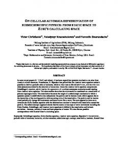
(a) Efficiency/C all graph of ECA rules at t = 1600.

the class III rules are rather crowded as compared with those of the class II rules. Symmetric and geometrical graphs are the networks of additive rules, and they are independent of their initial configuration. Some class II rules of ECA and class IV rules of 5TCA radically change their connections depending on the time steps and/or the initial configurations. Our preliminary results of the coefficient of variation for efficiency show that the unstable rules have large values of the coefficient than other rules. As examples, we have shown a time evolution of rule T20 network and sample networks of rule 184 obtained from pseudo-randomly generated initial configurations in Tables II and III, respectively. As discussed in [1], class II and III rules can be distinguished by their efficiency and dependency on the grid scale. The CC components, the probability of local clustering, can also be used to characterize each rule. The efficiency and C all of networks derived from the ECA and 5TCA rules are illustrated in Fig. 1. The class II rules of ECA seem to be separated into two types, “II-a” and “II-b,” which have estimated zero and nontrivial C all values, respectively. Unstable rules, such as rule 184 [24], are contained in the II-b rules of ECA and have greater efficiency than the other class II rules. The class III rules are plotted within the high efficiency/C all region. For the class IV rules, rule 110 lies in the region between classes II and III, whereas rules T20 and T52 (the diminished-radix complement of T11) are located at separate edges of the class II-b region. A radar chart of efficiency and CC components serves as a useful tool for studying the connectivity of an individual network. Sample charts of the independent ECA and 5TCA rules are listed in Table IV. Some typical graphs of these charts are summarized in Table V. The difference between classes II-a and II-b is illustrated by the clear contrast between their corresponding figures. Characteristics of the unstable class II-b rules are represented by a large C in relative to the other CC components. The instability of these rules can be explained intuitively from their degrees of distribution. As an example, the sampled inand out-degree distributions of rule 184 are shown in Fig. 2,

(b) Efficiency/C all graph of 5TCA rules at t = 800.

Figure 1: Efficiency/C all graph of networks derived from ECA and 5TCA rules, representing the average of networks obtained from ten pseudo-randomly generated initial configurations with N = 3201.

which illustrates that kiin and kiout have a high probability to be two and three, respectively. Therefore, the denominator of Ciin in Table I is smaller than those in the other components. Although these discrete distributions are easily changeable based on the choice of initial configuration, such tendency of Ciin is nearly maintained. On the other hand, the numerators of all components have strong randomness. Consequently, the mean value of C in becomes larger than the other components. In contrast, although rule T30 of 5TCA has a similar figure, shown in Table IVb, its parameters are relatively constant. This inconsistency is resolved by the degree distribution of rule T30 in Fig. 3 because its continuous distributions are not greatly affected by the choice of initial configuration. In our previous paper, we reported a scale-free behavior of the in-degree distribution of a rule T20 network (Fig. 4b). The radar chart of rule T20 in Table IVb is characterized by larger

198

Table IV: Sample radar charts of efficiency-CC components of networks derived from ECA and 5TCA rules, representing the average of ten sampled networks with N = 3201. The five axes are (clockwise from the top) efficiency, C cyc , C mid , C in and C out .

rule 1

rule 2

rule 3

rule 18

rule 22

rule 30

rule 54

rule 60

rule 73

rule 90

rule 110

rule 184

Table V: Typical figures of efficiency-CC component radar charts and their network connectivity. The rules inside the square brackets are the diminished-radix complement to the one outside the brackets.

(a) Sample radar charts of ECA rules at t = 1600.

rule T1

rule T2

rule T5

rule T10

rule T20

rule T30

rule T42

rule T52

(b) Sample radar charts of 5TCA rules at t = 800.

(a) P (kin ) of rule 184.

(b) P (kout ) of rule 184.

Figure 2: In- and out-degree distribution of a rule 184 network obtained from a pseudo-randomly generated initial configuration with N = 6401 and t = 3200.

(a) P (kin ) of rule T30.

(b) P (kout ) of rule T30.

Figure 3: In- and out-degree distribution of a rule T30 network obtained from a pseudo-randomly generated initial configuration with N = 6401 and t = 1600.

199

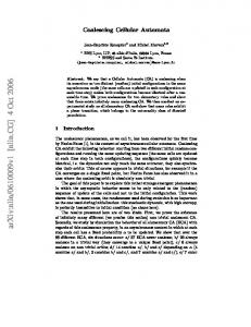
(a) P (kin ) of rule T8.

(a) P (kout ) of rule T20.

(b) P (kin ) of rule T20.

(b) P (kout ) of rule T24.

Figure 6: Non-averaged out-degree distributions of networks of rules T20 and T24 obtained from ten pseudo-randomly generated initial configurations with N = 6401 and t = 1600.

V. C ONCLUSIONS

(c) P (kin ) of rule T24.

(d) P (kin ) of rule T40.

Figure 4: Non-averaged in-degree distributions of four 5TCA rule networks obtained from ten pseudo-randomly generated initial configurations with N = 6401 and t = 1600.

(a) Radar chart of E. coli.

(b) P (kin ) of E. coli.

Figure 5: In-degree distribution of E. coli and its efficiencyCC components chart obtained from a biochemical reaction database [31].

values of C out and C mid than in the other components. Some class II rules have similar figures: rules 19, 23 and 36 of ECA, and rules T8, T24 and T40 of 5TCA. Among these rules, the three 5TCA rules show scale-free behavior, as demonstrated in Fig. 4. Fig. 5a shows a similar chart obtained from a scalefree network in the real-world, a metabolic network of E. coli, which was obtained from a biochemical reaction database [31] derived from the KEGG LIGAND database [32, 33]. The difference between rule T20 of class IV and other scale-free rules of class II is revealed in their out-degree distributions. As we can see in Fig. 6, the class IV rule has a greater variety of nodes with different out-degrees than the class II rules, which correspond to the complex dot patterns with log transients.

Our network representation has made it possible to show the dot patterns of CA using network graphs. Each graph has a characteristic connection pattern derived from the dynamical behavior of the corresponding CA rule. The graphs of the class III rules are quite crowded compared to those of the class II rules. The additive rules have symmetric and geometrical graphs that are independent of their initial configuration. Moreover, the rules forming a self- and diminished radix-complement pair have the same network representation. Because the efficiency and CC-components represent global and local connection structures, respectively, these parameters provide valuable indices for the classification of CA rules. A graph of the efficiency and CC-all component shows a distribution of rules related to their connection structures, which reveals another aspect of Wolfram’s classification, i.e., the class II rules are split into two categories, II-a and IIb. Class II-b includes some rules that radically change their network connections, depending on their initial configurations. The class IV rules are located between the class II and III regions or at the edges of the class II region. The characteristics of the derived networks are more clearly illustrated using radar charts of their efficiency and other CCcomponents. We discovered some characteristic figures, not only of each Wolfram’s class but also of unstable rules and those with a scale-free degree distribution. The common figure of scale-free networks has been confirmed using a real-world network, a metabolic network of E. coli. This figure has led us to other scale-free examples in 5TCA class II rules. The class IV and II rules of a scale-free nature can be distinguished by their out-degree distributions. The class IV rule (T20) has more complex distribution than those of the class II rules. As shown above, our network representation has brought about a way to investigate CA using network theory. This has led to remarkable but indistinct features: the separated positions of the class IV rules, shown in Fig. 1, and the appearance of scale-free distributions in networks derived from the class II and IV rules. Although our representation presents many samples of directed networks from CA rules, there are

200

a few examples of class IV rules in ECA and 5TCA. Further investigation into the above subjects and the relation between scale-free behavior and “the edge of chaos” requires further samples of class IV rules and their network representations. ACKNOWLEDGMENT I would like to thank Yasumasa Imamura for his valuable discussions. I also appreciate the feedback given by the three reviewers. In particular one of them gave insightful comments and suggestions. A PPENDIX All non-trivial network graphs of ECA and 5TCA rules are shown in Table VI. The initial configurations of each of the 41 cells are pseudo-randomly generated, and their time steps are set as 20 and 10 for ECA and 5TCA, respectively.

R EFERENCES [1] Y. Kayama, Complex networks derived from cellular automata, arXiv:1009.4509, 2010. [2] J. von Neumann, The theory of self-reproducing automata, in: A. W. Burks (Ed.), Essays on Cellular Automata, University of Illinois Press, 1966. [3] S. Wolfram, Theory and Applications of Cellular Automata, World Scientific, Singapore, 1986. [4] P. B. Hansen, Parallel cellular automata: A model program for computational science, Concurrency: Practice and Experience 5 (1993) 425–448. [5] G. B. Ermentrout, L. Edelstein-Keshet, Cellular automata approaches to biological modelling, J. Theor. Biol. 160 (1993) 97–133. [6] N. Ganguly, B. K. Sikdar, A. Deutsch, G. Canright, P. P. Chaudhuri, A Survey on Cellular Automata, Tech. Rep., Centre for high performance computing, Dresden University of Technology, 2003. [7] B. Chopard, M. Droz, Cellular Automata Modeling Of Physical Systems, Cambridge University Press, 2005. [8] S. Wolfram, Statistical Mechanics of Cellular Automata, Rev. Mod. Phys. 55 (1983) 601–644. [9] N. Ollinger, Universalities in cellular automata a (short) survey, in: B. Durand (Ed.), JAC, MCCME Publishing House, Moscow, ISBN 978-5-94057-377-7, 102–118, 2008. [10] A.-L. Barabási, R. Albert, Emergence of Scaling in Random Networks, Science 286 (1999) 509–512. [11] D. J. Watts, S. H. Strogatz, Collective Dynamics of Small-World Networks, Nature 393 (1998) 440–442. [12] S. Wasserman, K. Faust, Social Network Analysis, Cambridge University Press, 1994. [13] H. Jeong, B. Tombor, R. Albert, Z. N. Oltvai, The LargeScale Organization of Metabolic Networks, Nature 407 (2000) 651–654. [14] H. Jeong, S. Mason, A.-L. Barabási, Z. N. Olivai, Lethality and centrality in protein networks, Nature 411 (2001) 41–42.

[15] R. Albert, H. Jeong, A.-L. Barabási, Diameter of the World-Wide Web, Nature 406 (1999) 378–381. [16] A.-L. Barabási, R. Albert, H. Jeong, Scale-Free Characteristics of Random Networks: The Topology of the World-Wide Web, Physica A 281 (2000) 69–77. [17] K. Sutner, Additive Automata on Graphs, Complex Systems 2 (1988) 649–661. [18] K. Sutner, De Bruijn Graphs and Linear Cellular Automata, Complex Systems 5 (1991) 19–30. [19] D. O’Sullivan, Graph-cellular automata: a generalised discrete urban and regional model, Environ. Plann. B 28 (2001) 687–705. [20] M. Aldana, Boolean dynamics of networks with scalefree topology, Physica D 185 (2003) 45–66. [21] M. Aldana, P. Cluzel, A Natural Class of Robust Networks, Proc. Natl. Acad. Sci. 100(15) (2003) 8710–8714. [22] C. Darabos, M. Giacobini, M. Tomassini, PERFORMANCE AND ROBUSTNESS OF CELLULAR AUTOMATA COMPUTATION ON IRREGULAR NETWORKS, Adv. Complex Syst. 10 (2007) 85–110. [23] C. Marr, M.-T. Hütt, Outer-totalistic cellular automata on graphs, Phys. Lett. A 373 (2009) 546–549. [24] S. Wolfram, A New Kind of Science, Wolfram Media, Inc., 2002. [25] V. Latora, M. Marchiori, Efficient Behavior of SmallWorld Networks, Phys. Rev. Lett. 87-90 (2001) 198701– 198704. [26] S. Boccaletti, V. Latora, Y. Moreno, M.Chavez, D.U. Hwang, Complex networks: Structure and dynamics, Physics Reports 424 (2006) 175–308. [27] G. Fagiolo, Clustering in Complex Directed Networks, Phys. Rev. E 76 (2007) 026107–026114. [28] S. E. Ahnert, T. M. A. Fink, Clustering signatures classify directed networks, Phys. Rev. E 78 (3) (2008) 036112, doi:10.1103/PhysRevE.78.036112. [29] W. Li, N. Packard, The Structure of the Elementary Cellular Automata Rule Space, Complex Systems 4 (1990) 281–297. [30] A. K. Das, A. Sanyal, P. Palchaudhuri, On characterization of cellular automata with matrix algebra, Inf. Sci. 61 (3) (1992) 251–277. [31] H. Ma, A.-P. Zeng, Reconstruction of metabolic networks from genome data and analysis of their global structure for various organisms, Bioinformatics 19 (2) (2003) 270– 277. [32] S. Goto, T. Nishioka, M. Kanehisa, LIGAND: chemical database for enzyme reactions, Bioinformatics 14 (1998) 591–599. [33] S. Goto, Y. Okuno, M. Hattori, T. Nishioka, M. Kanehisa, LIGAND: database of chemical compounds and reactions in biological pathways, Nucleic Acids Res. 30 (2002) 402–404.

201

Table VI: Non-trivial networks of the ECA and 5TCA rules obtained from pseudo-randomly generated initial configurations with N = 41. The rules inside the square brackets are the diminished-radix complement to the one outside the brackets.

1

2

3

4

5

10

11

12

13

14

22

23 [232]

24

25

30

33

34

42

43

57

77 [178]

6

7

9

15 [240]

18

19

26

27

28

29

35

36

37

38

41

44

45

46

50

54

56

58

60

62

72

73

74

76

78

90

94

104

105 [150]

106

108

110

122

126

130

132

134

138

140

146

152

154

156

162

164

172

184

(a) Networks of ECA rules at t = 20.

200

T1

T2

T3

T5

T6

T7 [T 56]

T8

T9

T 10

T 11 [T 52]

T 12

T 13

T 14

T 17

T 18

T 20

T 21 [T 42]

T 22

T 24

T 25 [T 38]

T 26

T 28

T 30

T 34

T 40

T 44

(b) Networks of 5TCA rules at t = 10.

202