Network Sampling and Classification: An Investigation of Network ...

NIH Public Access Author Manuscript Decis Support Syst. Author manuscript; available in PMC 2012 June 01.

NIH-PA Author Manuscript

Published in final edited form as: Decis Support Syst. 2011 June ; 51(3): 506–518. doi:10.1016/j.dss.2011.02.014.

Network Sampling and Classification:An Investigation of Network Model Representations Edoardo M. Airoldia, Xue Baib, and Kathleen M. Carleyc aDepartment of Statistics, Harvard University, Cambridge, MA 02138, USA bSchool

of Business, University of Connecticut, Storrs, CT 06269, USA

cSchool

of Computer Science, Carnegie Mellon University, Pittsburgh, PA 15213, USA

Abstract


Methods for generating a random sample of networks with desired properties are important tools for the analysis of social, biological, and information networks. Algorithm-based approaches to sampling networks have received a great deal of attention in recent literature. Most of these algorithms are based on simple intuitions that associate the full features of connectivity patterns with specific values of only one or two network metrics. Substantive conclusions are crucially dependent on this association holding true. However, the extent to which this simple intuition holds true is not yet known. In this paper, we examine the association between the connectivity patterns that a network sampling algorithm aims to generate and the connectivity patterns of the generated networks, measured by an existing set of popular network metrics. We find that different network sampling algorithms can yield networks with similar connectivity patterns. We also find that the alternative algorithms for the same connectivity pattern can yield networks with different connectivity patterns. We argue that conclusions based on simulated network studies must focus on the full features of the connectivity patterns of a network instead of on the limited set of network metrics for a specific network type. This fact has important implications for network data analysis: for instance, implications related to the way significance is currently assessed.

Keywords


connectivity pattern; network type; network metrics; network sampling; network classification

1. Introduction Data about connections among individual entities arise in many areas such as management sciences [22; 36; 6], medical and biological sciences [14], and social, economic and information sciences [26; 24; 16; 31; 25]. Evidence from research and practice suggests that patterns of connectivity, rather than the intensity of interactions, drive productivity and other important aspects of collective behavior. A connectivity pattern is intuitively defined in terms of a special arrangement of connections among a set of nodes in a network.

© 2011 Elsevier B.V. All rights reserved [email protected] (Edoardo M. Airoldi), [email protected] (Xue Bai), [email protected] (Kathleen M. Carley). Publisher's Disclaimer: This is a PDF file of an unedited manuscript that has been accepted for publication. As a service to our customers we are providing this early version of the manuscript. The manuscript will undergo copyediting, typesetting, and review of the resulting proof before it is published in its final citable form. Please note that during the production process errors may be discovered which could affect the content, and all legal disclaimers that apply to the journal pertain.

Airoldi et al.

Page 2


Connectivity patterns are also referred to as characteristics of a network type and can be quantitatively characterized in terms of network metrics. For example, networks with six degrees of separation, also known as small-world networks, are typically characterized quantitatively in terms of two network metrics: network diameter and clustering coefficients. The typical connectivity pattern in a small-world network is one where, intuitively, nodes have many local connections and a few long-distance connections according to some given distance measure. Commonly seen network types include ring-lattice, small-world, scalefree, core-periphery, and random networks. There are 47 network metrics widely adopted in the social and physical sciences. Examples of popular network metrics include a variety of centrality measures, clustering coefficients, connectedness, hierarchies, and average distances [39].

Algorithm-based approaches to sampling networks [40; 34; 3] have received a great deal of attention in recent literature [9; 15; 30; 11; 41]. Most of the algorithms for sampling networks are based on simple intuitions. These algorithms associate only one ortwo connectivity patterns of an observed network—such as degree distribution, or diameter and clustering coefficient—with a simple process that aims to generate networks with the desired connectivity pattern [20].


However, current approaches have a number of issues. For example, the association between published algorithms and the connectivity pattern they are meant to generate has not been formally analyzed in the literature. The efficiency and robustness of these algorithms in generating networks with the desired connectivity patterns have not been quantified. Moreover, the association between these algorithms and the full set of network metrics of the networks they can generate has not been explored.


Typically, the structure of a network is defined as , in which is a set of nodes that represent individual entities, and is a set of edges that represent the connectivity pattern among the nodes. The connectivity pattern can be characterized by a popular set of network metrics, including measures of centrality of individuals, degree-based metrics, and global network metrics. Practitioners, however, rely on a limited subset of these network metrics to quantify structural patterns of network types of interest [3]. The disconnect between the limited network metrics that most sampling algorithms consider and the full set of network metrics that a network entails has important implications for network data analysis. For example, many empirical analyses implicitly assume that there is an association between a single metric and a type of networks. An analysis would then claim, for example, that scale-free networks are characterized by having a power-law degree distribution [40]. The substantive conclusions of this analysis crucially depend on the implicit assumption that one individual metric completely determines the structure of scalefree networks. Similarly, high clustering coefficient and low network diameter are believed to completely determine the structure of small-world networks [5]. In contrast, recent results have shown how it is possible to generate small-world networks with scale-free distribution, as well as scale-free networks with high clustering coefficient and low diameter [21]. Thus, in general, the problematic issue is that empirical and theoretical studies often claim that an observed network has a certain topological structure. However, the analyses that support such claims are often restricted to one or two network metrics. This is reasonable only if two conditions are met: 1) that one can assume the association between the algorithms and the topological structure is one-to-one, or approximately so; and 2) that the network metrics under consideration fully determine the topological structure of a network. These conditions are often not met. Another set of issues is related to the existence of multiple algorithms to generate the same type of networks. For instance, there are multiple papers dealing with small-world networks,

Decis Support Syst. Author manuscript; available in PMC 2012 June 01.

Airoldi et al.

Page 3


each one proposing an algorithm to generate small-world networks where nodes live in different metric spaces: on a ring-lattice [40] or in the plane [28]. How similar are the networks generated by these algorithms if we represent the sampled networks in terms of the currently available metrics? In this paper, we formally assess the extent to which alternative algorithms for generating the same network type actually generate networks with equivalent connectivity patterns; we refer to this issue as the stability issue. We also assess the extent to which different network types defined in terms of the commonly used network metrics actually display distinguishable connectivity patterns; we refer to this issue as the separability issue. In performing these assessments, we build on earlier work by Airoldi and Carley [3]. We expand their design of experiments and perform both qualitative and quantitative analyses of the stability of different network sampling methods and those of the separability of different network types. In addition, we discuss the statistical issues involved in network model selection such as sufficiency, and the implications of our findings for parameter estimation and p-value computation for network metrics. These are our key contributions to network analysis literature. 1.1. Brief Overview of Analyses and Results


We find that the popular network sampling algorithms, e.g., those for scale-free and smallworld networks, generate networks with similar connectivity patterns for non-pathological values of the relevant underlying constants. Furthermore, we find that alternative algorithms that supposedly generate networks with non-distinguishable connectivity patterns (e.g., algorithms for scale-free networks by different authors) actually give easily distinguishable connectivity patterns. These findings prompt us to make recommendations on how to provide successful assessments of the sensitivity of an analysis, to the connectivity patterns of different network types. Our findings also suggest that real-world networks may be better modeled as mixtures of these popular network types.

2. Problem Definition In this section we give a brief overview of the mathematical characteristics of a network, introduce our research context, and formally frame the research questions. 2.1. Mathematical Characterizations of a Network


A network G is defined by a set of N vertices, , and a set of edges, . The network G is fully specified by the adjacency matrix, Y, where the element Y(n, m) ε {0,1}, where 1 indicates a directed connection from node n to node m, i.e., n → m; 0 indicates that there is no such connection. The matrix Y encodes the connectivity patterns of the network it represents. We refer to those functions that map Y to scalar values as network metrics. For instance, the degree of a node is a node-specific metric, meaning every node has a degree measure; the density of a network is a global metric, meaning a network has a single density measure. For example, consider a binary network, the degree of the binary network is defined as

The density of the binary network is defined as


Airoldi et al.

Page 4


A collection of metrics induced from the adjacency matrix Y provides a quantitative representation of the connectivity patterns of the corresponding network G. In this sense, Y fully characterizes the values of the metrics on G. However, the contrary is not necessarily true. From a data analysis perspective, we would like to characterize a network in terms of its essential connectivity patterns in the space of metrics to maintain interpretability of the results. In fact, a number of metrics have been proposed in the quantitative psychology and social sciences literatures, and are based on well-established theories of individual and collective behavior [39; 12]. 2.2. Research Problems


The utility and appeal of sampling algorithms stems from the assumption that these algorithms are guaranteed to generate the desired connectivity patterns. For example, the “six degrees of separation” among individuals observed by [33] is captured by the “smallworld” network of [40]. This connectivity pattern informs the sampling algorithm that “individuals form local acquaintances, few of which relocate to places far away.“ This stylized model of behavior is sufficient to replicate the phenomenon observed by [33], and it “sounds” like a plausible explanation [33; 40]. Therefore we have the following research problem. Problem 1. (Sampling) Given algorithms that generate networks of the same type, we want to assess the stability of the connectivity patterns of the networks generated by these algorithms. Sampling algorithms can be both deterministic and probabilistic, and they typically depend on a small set of parameters. To fully evaluate their validity, it is important to provide ways to estimate such parameters from observed data.


A related problem, on the other hand, is that of determining which type we should assign to a network under analysis. Network types are used by practitioners to this extent. For example, homeland security officers are interested in determining whether an observed criminal network is cellular,given partial measurements about the network. If so, the conclusion may be drawn that destabilization strategies that are successful in cellular networks will be successful in destabilizing the given network. Hence we have the second research question. Problem 2. (Classification) Given algorithms that generate networks of different types, we want to assess the separability of the connectivity patterns of the networks generated by these algorithms. In the same example of the “homeland security” scenario, in order for officers to determine the correct network type of the criminal network under investigation, it is important for the connectivity patterns of the same network type to be stable and for those of different network types to be separable. We define a connectivity pattern to be stable if the networks sampled using algorithms for the same network type are similar in some metric space. We define connectivity patterns to be separable if the networks sampled using algorithms for


Airoldi et al.

Page 5

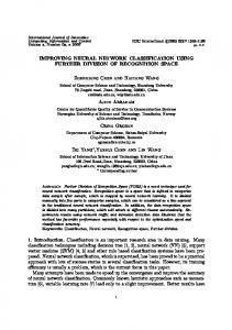
different network types are far apart in some metric space. Figure 1 shows an illustrative example of the two research questions.


The goal of sampling networks (left) is to assess the consistency of alternative algorithms to generate the same type of networks. The larger the intersection between the supports, the more consistent alternative definitions are—since they cannot generate many different networks. The goal of classifying networks (right) is to assess the need for defining alternative types of networks. The smaller the intersection between the supports, the less confounded different types of networks are—this is because the generated networks are different enough to be distinguishable. The reference space used in this paper is defined by 47 metrics [39]. We project all sampled networks in this space. The stability property of alternative sampling algorithms for the same network type guarantees that choosing one specific algorithm over another does not affect the validity of the conclusions. The separability property of alternative sampling algorithms for different network types guarantees that any set of observed connectivity patterns identifies a unique network type. In other words, separability suggests that it is logically possible to answer questions such as “Is the given network of type X?” The experiments in section 3.3 are devoted to assess stability and separability of the sampling algorithms surveyed or introduced in section 3.1.


3. Experimental Design The two research problems we tackle are: (1) stability, i.e., to what extent different sampling algorithms for the same pure network type lead to consistent connectivity patterns, as captured by the set of network metrics, and (2) separability, i.e., to what extent the classification of an observed network mapped into the reference space of metrics can uniquely determine the pure network types. In this section, we begin by the heuristic descriptions of the six network types that are commonly seen in network analysis. We then discuss the set of network metrics used in our experiments. After that, we present the experimental setting and the classification scheme. 3.1. Network Types Sampled Type 1. (Ring Lattice) Each node is connected to its neighbors, according to the ringinduced distance (Figure 2). Type 2. (Small World) Each node is connected to several of its neighbors and a few distant nodes, according to the ring-induced distance [40] (Figure 3).


Type 3. (Erdös-Rényi-Gilbert Random) Each node is connected to a random set of the remaining nodes [17; 19; 8] (Figure 4). Type 4. (Scale Free) Most of the nodes are connected to a few other nodes, while a small number of nodes are connected to many other nodes. This relation is formally described with a power law, between the number of edges and the number of connections [5] (Figure 5). Type 5. (Cellular) Nodes are divided into cells. Connections are frequent between nodes within each cell, and rare between nodes in different cells [18] (Figure 6). Type 6. (Core-Periphery) Nodes belong exclusively to either the core or the periphery. Core and periphery nodes are connected to core nodes, while there are no edges among periphery nodes [10](Figure 7). Table 1 presents a summary of the algorithms that we consider in the present study. Decis Support Syst. Author manuscript; available in PMC 2012 June 01.

Airoldi et al.

Page 6

3.2. Network Metrics Used


We focused our analysis on the 47 metrics that are widely adopted in the social and physical sciences [39]. These metrics are: degree centrality (no.1–41), which measures the centrality of a node in terms of its degree distribution; betweenness centrality (no.5–8), which measures the centrality of a node in terms of the shortest paths of which the node is a member; closeness centrality (no.9–12, inverse closeness centrality (no.13–16), eigenvector centrality (no.17–20), clustering coefficient (no.21–24, density of the connectivity around a node), effective network size (no.25–28), network constraint (no.29–32), node levels (no. 33–36), triad count (no.37–40), global efficiency (no.41), local efficiency (no.42), efficiency (no.43), connectedness (no.44), hierarchy (no.45), upper boundedness (no.46), and average distance (no.47). Formal definitions are available in [39]. The detailed descriptions of the metrics we used are available in [12]. 3.3. Performing Sampling and Classification


A few of the network metrics we consider depend on the size and the average connectivity of a network; for instance, the degree distribution and the triad counts. In order to obtain results and substantiate claims that are independent from these network characteristics, we fix network size and average connectivity in our experimental design. For each of the six network types, we set an evenly spaced grid that spans the entire parameter space. We sampled at least ten networks for each parameter configuration. The algorithms with more parameters have more possible configurations, and result in a larger sample of networks— which we control for in the experiments using stratified five-fold cross-validation scheme, which are detailed in the next two paragraphs. In addition, we control for other relevant parameters when generating the same network type using different algorithms, with the goal of making sampled networks of the same type consistent across the alternative generating algorithms. Full specifications of the experimental design are detailed in Table 2. We choose the naïve Bayes classifier as the classifier. Naïve Bayes classifier has been shown to be the most accurate in predicting the network type of a given network [4]. The classification procedure is as follows. For a given network, we examine the connectivity patterns as captured by the set of 47 metrics we consider. We sample a large quantity of networks, with different parameter values for each pure type. For each sampled network, we first compute the corresponding metrics, then classify it into a network type according to the posterior probability of types given its metrics configurations. We use classification errors to indicate the degree to which pairs of pure network types overlap in the reference space of metrics, see Figure 1.


In order to estimate the classification errors we use a stratified five-fold cross validation scheme. Five-fold cross validation step aims at estimating error on out-of-sample networks. It consists of the following procedure: we split the set of sample networks into five mutually exclusive batches, we then iteratively (i = 1,‖,5) train naïve Bayes classifier on four batches and test on the ith one, and finally we estimate the prediction error using the average prediction errors on the five-folds. The stratification step makes sure that in each training set there are networks of each type, despite some types being more abundant than others in the design. The proportions of networks of each type in the training set are the same as the proportions of networks of each type in the overall sample. The stratification aims at minimizing the potential over-fitting in the estimated accuracy [23].

1Whenever a metric is associated with four indices, it means that we derived four statistical quantities related to it. These quantities are the minimum, the maximum, the average, and the standard deviation, respectively.


Airoldi et al.

Page 7

4. Computational Results NIH-PA Author Manuscript

Here we present quantitative and qualitative analyses to explore the stability and separability issues that arise in the classification problem introduced in Section 2.2. 4.1. Qualitative Assessment of Stability To assess the variability in the network metrics of the sampled networks by alternative sampling algorithms, for each type of the network, we report the comparative empirical distributions of the 47 metrics by each of the alternative sampling algorithms. Figures 8–12 present the comparative results for five network types: random, cellular, scale-free, coreperiphery, and small-world, respectively. Since there are no alternative algorithms to generate ring-lattice networks, we did not report those histograms. The empirical distributions in these figures were estimated using kernel density estimator, which estimates a continuous histogram using a sliding window and a function, the kernel, to weigh the contribution of different points in the window [38]. Each figure consists of 47 panels; each panel corresponds to a metric, clearly labeled at the top of each panel. Within each panel, we plot multiple density estimates in different colors; each color representing one of the alternative sampling algorithms for a network type. A legend that specifies the corresponding color for each sampling algorithm in Table 2 is given in the bottom right panel of the figure.


The comparison of each metric provides a first look at the consistency of alternative sampling algorithms. As described in Section 2.2 and illustrated in the left panel of Figure 1, we want to assess the consistency of alternative algorithms to generate the same type of networks. A large overlap among the network instances by alternative sampling algorithms is desirable, since it would suggest consistency of the alternative algorithmic definitions of a network type. In the context of Figures 8–12, similar distributions for each of the metrics is desirable, since it would suggest consistency of alternative definitions of the same network type. However, as shown in the panels, almost all of the metrics distributions are different to various degrees. For example, in the random networks (Figure 8), 45 out of 47 metrics distributions are vastly different. The only two that are similar are the standard deviation of betweenness centrality (the eighth panel on the top row) and the maximum eigenvector centrality (the second panel on the third row from the top). Similar assessments can be conducted based on the distributions in Figures 9–12. The lack of similarity we see in these Figures suggests that alternative definitions of network types are not consistent.


More specifically, Figure 8, for example, displays the empirical distributions for the 47 metrics computed on the random networks generated using algorithms 3.1 (np) and 3.2 (nm). Here “np” stands for the two parameters, n and p, that algorithm 3.1 uses as inputs; n and m are the two parameters that algorithm 3.2 uses as inputs. The set of parameter values used to generate the network samples are specified in Table 2. As an illustration, the fourth panel on the top row describes the empirical distributions of the standard deviation of the node degrees for algorithms 3.1 and 3.2. The distribution in green corresponds to algorithm 3.1. The distribution in red corresponds to algorithm 3.2. As expected, the standard deviation of the node degree is much smaller for the networks generated with algorithm 3.2, because this algorithm leads to networks that have the same exact average connectivity whenever the same value of the parameter (the number of connections m in this case) is used. The red distribution of standard deviation reflects changes in the parameter values detailed in Table 2. The green distribution of the standard deviation, which corresponds to networks generated with algorithm 3.1, reflects both changes in the parameter values and a higher variability of the node degrees due to the design of algorithm 3.1 itself.


Airoldi et al.

Page 8

4.2. Quantitative Assessment of Stability


Next, we assess the stability of connectivity patterns of the network types to the alternative algorithms used to generate networks of a given type. The values reported are five-fold cross-validated errors in a classification task: the lower the error is, the less stable connectivity patterns are, since a slight variation in the sampling algorithm leads to distinguishable sets of measurements. Random—Using the set of metrics, we can discriminate almost exactly which type of network was generated by which algorithm. The extremal statistics (min, max) are very powerful discriminators in this case. The area under the Receiver Operating Characteristic (ROC) curve is about 1 and the classification error about is 0.00%. Core Periphery—Using the set of metrics, we cannot discriminate which type of network was generated from which algorithm. The classification error is about 50% and the area under the ROC curve is 0.501. Cellular—Using the set of metrics, we can discriminate fairly well which type of network was generated from which algorithm. The area under the ROC curve is 0.928 and the classification error is 17.64%.


Scale Free—Using the set of metrics, we can discriminate almost exactly which type of network was generated from which algorithm. The area under the ROC curve is about 1 and the classification error is 0.07%. Small World—Using the set of metrics, we can barely discriminate which type of network was generated from which algorithm. The area under the ROC curve is not available because this is a three-way classification problem. The three-way classification error is 24.78% (the base error is at 33.33%). Pairwise classification errors are presented in Table 3. Compared to the base error rate of 50%, the pairwise classification results suggest that the any pair of the alternative sampling algorithms yield distinguishable sets of small-world networks. 4.3. Qualitative Assessment of Separability


To explore the variability in the network metrics induced by different network types, we look at the empirical distributions of the 47 metrics without distinguishing which networks were generated by which algorithms, in Figure 13. This Figure has 47 panels, each panel corresponding to a metric, clearly labeled at the top as in the previous set of Figures. In each panel, we plot multiple density estimates in different colors, each density corresponding to one of the network types, without distinguishing the sampling algorithm used. A legend that specifies which color corresponds to which network type in Table 2 is given in the bottom right panel. This analysis provides a first look at the separability issue of network types, as described in Section 2.2 and illustrated in the right panel of Figure 1 and to what extent algorithms for a new network type actually generate networks (in terms of their connectivity properties) that existing network types cannot generate. In the right panel of Figure 1 a small intersection would be desirable, as it would suggest a substantial difference among the six network types we consider. In the context of Figure 13, a small intersection in the distributions for each of the metrics would be desirable, as the differences would lead to better separability among network types. However, the plots in Figure 13 show that such differences are distinguishable in some metric distributions (e.g., the average degree centrality, connectedness, and hierarchy) while similar in others (e.g., the standard deviation of inverse


Airoldi et al.

Page 9

centrality, max closeness centrality), suggesting that different network types are only separable in terms of some network metrics, not in others.


As a specific example, in Figure 13, the third panel on the top row plots six empirical distributions of average degree centrality corresponding to the six network types we consider. This measure of centrality takes very different values across network types, which suggests that the six network types are different in terms of those properties of the connections that influence degree centrality. However, this metric is one of the few metrics with respect to which the network types are fairly different. The six distributions tend to be more similar than not in most of the other panels. For instance, consider the clustering coefficient in the seventh panel on the third row, or the effective network size in the fifth panel on the fourth row. According to these metrics the network types are not very different. This suggests that the six network types are more similar than not in terms of those properties of the connections that influence most metrics. 4.4. Quantitative Assessment of Separability


Finally, we assessed the separability of sampling algorithms for different network types. Table 4 summarizes the five-fold cross-validated errors in the corresponding classification tasks. Diagonal cells replicate the stability results discussed above. Off-diagonal cells quote separability results. The lower the error is, the more separable connectivity patterns are, since the instances of different pure types entail distinguishable sets of metrics. In Table 4, we quote the cross-validate classification errors. The off-diagonal element (i, j) is the error in classifying networks of type i from networks of type j. Since network types i and j are different for off diagonal entries, low error is desirable. It means that network types i and j are separable. The diagonal element (i, i) is the error in classifying networks of type i generated with different sampling algorithms. Note that the top-left element (RL, RL) is not available, since we only consider one sampling algorithm for regular lattice networks. Since there is only one network type i for diagonal entries, high error is desirable. It means that networks generated by alternative sampling algorithms are not separable, thus leading to a consistent definition of the network type.


Table 4 suggests that cellular, core-periphery and scale-free types are weakly separable (26.45%, 33.33% and 37.15% error), and share common connectivity patterns with random types (2nd row; 27.94%, 32.55%, and 25.00%). These types are separable from small-world networks (3rd row, 8.66%, 13.12%, and 5.31%) that, in turn, share a set of different connectivity patterns with random types (41.22%). Note that, key differences between cellular, core-periphery, scale-free and random are that (a) the differences are more apparent at moderate density (apx. 25% range) and (b) certain metrics can be used to separate these four types of networks.

5. Discussion The computational results on stability suggest that all of the studied network sampling methods are fairly simple. These methods may entail “no variability” for a specific metric over a fairly large range of parameter values, or by construction, e.g., all instances of an Erdös random (n, m) have the same number of edges, i.e., m. While these algorithms are of theoretical value and help us grasp insights about phenomena of interest, they may lead to unreliable statistical tests (e.g., highly variable p-values) in practice. This is because rich variability profiles are crucial in determining the stability of connectivity patterns of a pure type to alternative sampling algorithms that generate it. In other words, low variability profiles lead to high sensitivity of connectivity patterns, as captured by the metrics of interest, and ultimately to high sensitivity of relevant statistics to the specific version of the Decis Support Syst. Author manuscript; available in PMC 2012 June 01.

Airoldi et al.

Page 10


algorithms adopted. For example, the variability profile of the clustering coefficient is extremely sensitive to the specific algorithm used to sample both random and scale-free types. As a consequence the p-value, e.g., of small-worldness, will vary. A simple suggestion to overcome this problem is to sample network types according to different algorithms, and then to mix the networks. This directly aims at increasing the variability profiles of the metrics of interest, and possibly leads to more robust parameter estimations.


Overall, we find low stability and low separability. Alternative sampling algorithms that we considered for the same type appear similar. Yet the connectivity patterns they yield are neither consistent to alternative algorithms, nor separable across different network types. The low stability (not desirable) is likely to be a consequence of the fact that the algorithms are too simple and do not lead to rich enough variability profiles for the metrics of interest. In fact, we find that the extremal statistics (min and max) have high information gain with respect to the network type categories, and drive the classification in several cases. The low separability (not desirable) means that pure types are stylized models of behavior at the sampling level, which lead to networks that share connectivity patterns, as captured by the network metrics of interest. Aside from the simplicity of the algorithms, this is consistent with what we would expect to see in the real world, i.e., observed networks display multiple stylized behaviors to different degrees. This translates into the more realistic hypothesis of “mixtures of types,” at the sampling level, as a better starting point for developing models and algorithms for network analysis. 5.1. Open Issues in Network Model Selection The problem we addressed in this paper is an instance of the network model selection problem in statistics, i. e., how to select a most appropriate network model M for an observed network G? A model M specifies a probability distribution PM(G | Θ) on space of possible networks G giving some parameters Θ. The model selection problem amount to determining which model best fits the observed network among a set of models. The current practice to select a network model is the following [e.g., see 32]. Consider an observed network G and a candidate statistical model M. The observed network is represented as a set of network metrics tM(G). Using these metrics, optimal values of the parameters are estimated, then a large number B of networks G1:B are generated from the


probability distribution ). Finally, an overall p-value of the observed network is computed. The overall p-value of the observed network is informative about how unexpected the connectivity pattern is, with respect to the expected pattern under the candidate model M. Lower p-values indicate that the observed network is more unusual under the model M. This sequence of steps is repeated for a set of models. The model that best fits the connectivity pattern of the observed network is chosen. There are two issues with the current practice outlined above. The procedures to estimate the optimal parameter values lack a sound statistical basis. The metrics used in the estimation procedure tM may not carry sufficient information about a candidate model M. To estimate optimal parameter values , for instance, a typical procedure identifies the values of the parameters that match the empirical values network metrics tM, such as average number of interaction per individual, to the expected value of these metrics computed using the candidate model M. The full specifications of probability distribution PM are used to compute expectations, thus linking Θ to the observed network data. A more principled estimation procedure would be to find the values of the parameters that best explain the observed network data, for instance, by maximizing the probability of the data PM(G | Θ) with respect to Θ. Another option would be to set expectations on the parameters Decis Support Syst. Author manuscript; available in PMC 2012 June 01.

Airoldi et al.

Page 11


in terms of a probability distribution P(Θ) to find the values of the parameters that are most likely given the data, by maximizing PM(Θ | G) with respect to Θ. These estimation procedures would correspond to maximum likelihood and maximum a-posteriori estimation [38]. Another fundamental issue is the choice of the metrics that quantitatively summarize the interaction data and inform the estimation of the parameters. In principle, we should estimate the parameters of a model PM(G | Θ) using a set of metrics uM(G) that are sufficient to characterize G [13]. That is, we should use metrics that carry all the information about the network that is necessary to estimate the parameters in a candidate model PM. Each model, PM corresponds to a specific set of metrics uM that are sufficient statistics. Statistical network analysis, however, is still in its infancy. It is often infeasible to compute or even write down the likelihood PM for a given model M. Often, we cannot tell what set of metrics uM is sufficient to estimate the parameters in a given model [29].


In practice, as reported above, each statistical model characterizes networks in terms of specific metrics tM(G). Community-based models, such as the cellular networks, portray interactions in which individuals work in tight teams, most often interacting with other team members and occasionally interacting with other teams [35]. Centralized models, such as core-periphery networks, portray interactions in which most individuals report to a central figure and seldom interact with one another [37; 1]. Current estimation practice leverages the purported correspondence between a given network model and a specific set of metrics tM. Parameters are estimated using only the information about the network captured by tM, according to the procedures outlined above. However, there may be a substantial difference between the information captured by the arbitrary set of metrics tM and the information captured by the metrics set uM, that is, tM may be highly insufficient for summarizing the information of an observed network. In the current literature, the metrics tM associated to models PM are typically one or two. The small-world model, for example, is characterized in the literature in terms of metrics tM quantifying diameter and clustering coefficient [40]. Estimating the parameters of the small-world model using the limited information captured by tM is problematic, and leads to unstable p-values and sub-optimal decisions.

6. Conclusion


In this paper, we performed statistical analysis of the stability of the network sampling methods and the separability of different network types as captured by a set of network metrics that are widely adopted in the social and physical sciences. Contrary to the widespread assumptions in research, we found that the sampling algorithms considered are neither stable to alternative specifications, nor separable in terms of the connectivity patterns they entail. The lack of stability is a cause for concern. We encourage the practitioners who employ the simple sampling algorithms discussed in this paper to consider more variable schemes, such as mixtures, in order to obtain more robust network modeling parameters in general. The lack of separability was somewhat anticipated, as real world networks hardly present the variability profile of a single pure network type. Our results support the assumption of mixtures of network types as an alternative starting point for developing models and algorithms for network analysis [e.g. 2]. Developing novel network metrics and exploring alternative network representations grounded in scientific theories are promising directions for future research, which may transform the way we do network analysis today.

Acknowledgments This work was partially supported by the National Institutes of Health under grant no. R01 AG023141-01, by the Office of Naval Research under contract no. N00014-02-1-0973, by the National Science Foundation under grant no. IIS-0218466, and by the Department of Defense, all to Carnegie Mellon University, and by the National


Airoldi et al.

Page 12


Science Foundation under grants no. DMS-0907009 and no. IIS-1017967, by the National Institute of Health under grant no. R01-GM096193, and by the Army Research Office Multidisciplinary University Research Initiative under grant no. 58153-MA-MUR all to Harvard University. Additional support was provided by the center for Computational Analysis of Social and Organizational Systems (CASOS) at Carnegie Mellon University. The views and conclusions contained in this document are those of the authors and should not be interpreted as representing the official policies, either expressed or implied, of the National Institute of Health, the Office of Naval Research, the National Science Foundation, or the U.S. government.

1 Biographical Note Dr. Edoardo M. Airoldi is an Assistant Professor of Statistics and Computer Science at Harvard University. He is also a member of the Center for Systems Biology in the Faculty of Arts and Sciences at Harvard University. He received a PhD degree in Computer Science from Carnegie Mellon University. He was postdoctoral fellow at Princeton University, in the Lewis-Sigler Institute for Integrative Genomics, and the Department of Computer Science. His research interests include statistical methodology and theory for the analysis of complex networks and random graph dynamics, with application to the social and biological sciences.


Dr. Xue Bai is an Assistant Professor of Management Information Systems in the Department of Operations and Information Management, University of Connecticut. She received her PhD degree in Management Information Systems from Carnegie Mellon University. Her research includes data mining and machine learning methods applied to text classification, sentiment extraction, online marketing analysis and clinic diagnosis. Another area of her research is in the application of optimization methods to data quality and information security associated risks in enterprise systems.


Dr. Kathleen M. Carley is Professor of Organizational Sociology at Carnegie Mellon University. She is the director of the center for Computational Analysis of Social and Organizational Systems (CASOS), a university wide interdisciplinary center that brings together network analysis, computer science and organization science (www.casos.ece.cmu.edu). She carries out research that combines cognitive science, dynamic social networks, text processing, organizations, social and computer science in a variety of theoretical and applied venues. Her specific research areas are computational social and organization theory; dynamic social networks; multi-agent network models; group, organizational, and social adaptation, and evolution; statistical models for dynamic network analysis and evolution, computational text analysis, and the impact of telecommunication technologies on communication and information diffusion within and among groups. She is the lead developer of ORGAHEAD, a tool for examining organizational adaptation, CONSTRUCT-TM, a computational model of the co-evolution of people and social Networks, DyNet, a computational model for network destabilization, BioWar a city-scale multi-agent network model of weaponized biological attacks, MECA and AutoMap which are computational tools for automated text analysis.

References [1]. Ahuja MA, Carley KM. Network structure in virtual organizations. Organization Science. 1999; 10(6):741–757. [2]. Airoldi EM, Blei DM, Fienberg SE, Xing EP. Mixed membership stochastic blockmodels. Journal of Machine Learning Research. 2008; 9:1981–2014. [PubMed: 21701698] [3]. Airoldi EM, Carley KM. Sampling algorithms for pure network topologies: Stability and separability of metric embeddings. ACM SIGKDD Explorations. 2005; 7(2):13–22. [4]. Airoldi, EM.; Cohen, WW.; Fienberg, SE. Bayesian models for frequent terms in text. Proceedings of the Classification Society of North America and INTERFACE Annual Meetings; 2005. [5]. Albert R, Barabasi AL. Statistical mechanics of complex networks. Reviews of Modern Physics. 2002; 74(47)


Airoldi et al.

Page 13

NIH-PA Author Manuscript NIH-PA Author Manuscript NIH-PA Author Manuscript

[6]. Bajaj A, Russell R. Awsm: Allocation of workflows utilizing social network metrics. Decision Support Systems. 2010; 50(1):191–202. [7]. Barabasi AL, Albert R. Emergence of scaling in random networks. Science. 1999; 286:509–512. [PubMed: 10521342] [8]. Bollobás, B. Random Graphs. 2nd edition. Academic Press; New York: 2001. [9]. Borgatti SP, Cross R. A relational view of information seeking and learning in social networks. Management Science. 2003; 49(4):432–445. [10]. Borgatti SP, Everett MG. Models of core / periphery structures. Social Networks. 1999; 21:375– 395. [11]. Carley KM, Diesner J, Reminga J, Tsvetovat M. Toward an interoperable dynamic network analysis toolkit. Decision Support Systems. 2007; 43(4):1324–1347. [12]. Carley, KM.; Reminga, J. Technical Report CMU-ISRI-04-106. Carnegie Mellon University; 2004. ORA: Organizational Risk Analyzer. [13]. Casella, G.; Berger, RL. Statistical inference. 2nd edition. Duxbury; 2002. [14]. Christakis, NA.; Fowler, JH. Connected: The Surprising Power of Our Social Networks and How They Shape Our Lives. Little, Brown and Company; 2009. [15]. Dodds PS, Watts DJ, Sabel CF. Information exchange and the robustness of organizational networks. Proceedings of the National Academy of Sciences. 2003; 100(21):12516–12521. [16]. Easley, D.; Kleinberg, J. Networks, Crowds, and Markets: Reasoning About a Highly Connected World. Cambridge University Press; 2010. [17]. Erdös P, Rényi A. On random graphs. Publicationes Mathematicae Debrecen. 1959; 5:290–297. [18]. Frantz, T.; Carley, KM. Technical Report CMUISRI-05-109, School of Computer Science. Canregie Mellon University; 2005. A formal characterization of cellular networks. [19]. Gilbert EN. Random graphs. Annals of Mathematical Statistics. 1959; 30:1141–1144. [20]. Goldenberg A, Zheng AX, Fienberg SE, Airoldi EM. A survey of statistical network models. Foundation and Trends in Machine Learning. 2010; 2(2):1–117. [21]. Handcock, MS.; Morris, M. Workshop on Statistical Network Analysis̀, Lecture Notes in Computer Science. Springer; 2007. A simple model for complex networks with arbitrary degree distribution and clustering; p. 103-114. [22]. Harary F. Graph theoretic methods in the management sciences. Management Science. 1959; 5(4):387–403. [23]. Hastie, T.; Tibshirani, R.; Friedman, JH. The Elements of Statistical Learning: Data Mining, Inference, and Prediction. Springer-Verlag; 2001. [24]. Jackson, MO. Social and Economic Networks. Princeton University Press; 2008. [25]. Keith M, Demirkan H, Goul M. The influence of collaborative technology knowledge on advice network structures. Decision Support Systems. 2010; 50(1):140–151. [26]. Kiss C, Bichler M. Identification of influencers – measuring influence in customer networks. Decision Support Systems. 2008; 46(1):233–253. [27]. Kleinberg, J. Technical Report 99-1776, Department of Computer Science. Cornell University; 1999. The small-world phenomenon: An algorithmic perspective. [28]. Kleinberg J. Navigation in a small world. Nature. 2000; 845 [29]. Kolaczyk, ED. Statistical Analysis of Network Data: Methods and Models. Springer; 2009. [30]. Kossinets G, Watts DJ. Empirical analysis of an evolving social network. Science. 2006; 311:88– 90. [PubMed: 16400149] [31]. Mayer A. Online social networks in economics. Decision Support Systems. 2009; 47(3):169–184. [32]. Middendorf M, Ziv E, Wiggins CH. Inferring network mechanisms: The drosophila melanogaster protein interaction network. Proceedings of the National Academy of Sciences. 2006; 102(9): 3192–3197. [33]. Milgram S. The small world phenomenon. Psychology Today. 1967; 1(61) [34]. Newman MEJ, Watts DJ, Strogatz SH. Random graph models of social networks. Proceedings of the National Academy of Sciences. 2002; 99:2566–2572.


Airoldi et al.

Page 14


[35]. Oh W, Jeon S. Membership herding and network stability in the open source community: The ising perspective. Management Science. 2007; 53(7):1086–1101. [36]. Shane S, Cable D. Network ties, reputation, and the financing of new ventures. Management Science. 2002; 48(3):364–381. [37]. Walker G, Kogut B, Shan W. Social capital, structurel holes and the formation of an industry network. Organization Science. 1997; 8(2):109–125. [38]. Wasserman, L. All of Statistics. Springer-Verlag; 2004. [39]. Wasserman, S.; Faust, K. Social Network Analysis: Methods and Applications. Cambridge University Press; 1994. [40]. Watts DJ, Strogatz SH. Collective dynamics of “small-world” networks. Nature. 1998; 393:440– 442. [PubMed: 9623998] [41]. Zhu B, Watts SA. Visualization of network concepts: The impact of working memory capacity differences. Information Systems Research. Jun; 2010 21(2):327–344.

NIH-PA Author Manuscript NIH-PA Author Manuscript Decis Support Syst. Author manuscript; available in PMC 2012 June 01.

Airoldi et al.

Page 15


Figure 1.

An illustration of the two research problems.


Airoldi et al.

Page 16

NIH-PA Author Manuscript NIH-PA Author Manuscript

Figure 2.

A ring-lattice network.

NIH-PA Author Manuscript Decis Support Syst. Author manuscript; available in PMC 2012 June 01.

Airoldi et al.

Page 17


Figure 3.

A small-world network.


Airoldi et al.

Page 18


Figure 4.

A random network.


Airoldi et al.

Page 19


Figure 5.

A scale-free network.


Airoldi et al.

Page 20


Figure 6.

A cellular network.


Airoldi et al.

Page 21


Figure 7.

A core-periphery network.


Airoldi et al.

Page 22


Figure 8. random

Empirical distributions of the 47 metrics we consider, excluding shortest path. The distributions were estimated using the sample of random networks generated by algorithms 3.1 (np) and 3.2 (nm) in the experimental design in Table 2.


Airoldi et al.

Page 23


Figure 9. cellular

Empirical distributions of the 47 metrics we consider, excluding shortest path. The distributions were estimated using the sample of cellular networks generated by to algorithms 6.1 (nkpq) and 6.2 (nkpqr) in the experimental design in Table 2.


Airoldi et al.

Page 24


Figure 10. scale-free

Empirical distributions of the 47 metrics we consider, excluding shortest path. The distributions were estimated using the sample of scale-free networks generated by algorithms 4.1 (nipi) and 4.2 (nmr) in the experimental design in Table 2.


Airoldi et al.

Page 25


Figure 11. core-periphery

Empirical distributions of the 47 metrics we consider, excluding shortest path. The distributions were estimated using the sample of core-periphery networks generated by algorithms 5.1 (npi-uni) and 5.2 (npi-prf) in the design in Table 2.


Airoldi et al.

Page 26


Figure 12. small-world

Empirical distributions of the 47 metrics we consider, excluding shortest path. The distributions were estimated using the sample of small-world networks generated by algorithms 2.1 (nkp), 2.2 (nklr) and 2.3 (nkpqr) in the design in Table 2.


Airoldi et al.

Page 27


Figure 13. Six network types

Empirical distributions of the 47 metrics we consider, excluding shortest path. The distributions were estimated using the entire sample of networks generated according to all the algorithms in the experimental design of Table 2.


Airoldi et al.

Page 28

Table 1

Summary of published and newly introduced generative algorithms.


Type

Algorithm

Parameters

Description of Parameters

1.1.

Ring Lattice [8]

Θ = (n, k)

nodes, neighbors

2.1.

Small World [40]

Θ = (n, k, pn)

nodes, neighbors, pr rewire

2.2.

Small World [27]

Θ = (n, k, l, r)

nodes, neighbors, distant nodes, power-law exp

2.3.

Small World

Θ = (n, k, pk, pn, r)

nodes, init neighbors, pr neighbor, pr distant nodes, power-law exp

3.1.

Random [17]

Θ = (n, pn)

nodes, pr edge

3.2.

Random [19]

Θ = (n, m)

nodes, edges

4.1.

Scale Free [7]

Θ = (n, n0, p0, pn)

nodes, init nodes, pr init edge, pr edge

4.2.

Scale Free

Θ = (n, m, r)

nodes, edges, power-law exp

5.1.

Core–Periphery [10]

Θ = (n, p0, p)

nodes, pr core nodes, pr edge

5.2.

Core–Periphery

Θ = (n, p0, p)

nodes, pr core nodes, pr edge

6.1.

Cellular [18]

Θ = (n, k, pk, pn)

nodes, pr in-node, cells, pr out-node

6.2.

Cellular

Θ = (n, k, pk, pn, r)

nodes, pr in-node, cells, pr out-node, power-law exp


Airoldi et al.

Page 29

Table 2

Design of experiments.


Type

Algorithm

1.1

Ring Lattice

Samples

2.1

Small World (rewire)

484

2.2

Small World (number)

1250

n = 250, k = 2, 4, .., 50, l = 1, 2, .., 10, r = 1, 2, .., 5

2.3

Small World (prob.)

2670

n = 250, k = 2, 4, .., 50, pk = 0.20, 0.30, .., 0.80, pn = 0.20, 0.30, .., 0.80, r = 1, 2, .., 5

3.1

Random (prob.)

17

n = 250, p = 0.10, 0.15, ..0.90

3.2

Random (number)

17

n = 250, m = 311, 622, .., 28012

4.1

Scale Free (pref.)

729

4.2

Scale Free (power)

45

n = 250, m = 311, 622, .., 28012, r = 1, 2, .., 5

5.1

Core-Periphery (uniform)

54

n = 250, p0 = 0.10, 0.20, .., 0.90, p = 0.25, 0.35, .., 0.75

5.2

Core-Periphery (pref.)

54

n = 250, p0 = 0.10, 0.20, .., 0.90, p = 0.25, 0.35, .., 0.75

6.1

Cellular (uniform)

360

n = 250, k = 2, 4, .., 20, pk = 0.25, 0.35, .., 0.75, pn = 0.25, 0.35, .., 0.75

6.2

Cellular (power)

360

n = 250, k = 2, 4, .., 20, pk = 0.25, 0.35, .., 0.75, pn = 0.25, 0.35, .., 0.75, r = 1

25

Parameter Configuration

n = 250, k = 2, 4, .., 50 n = 250, k = 2, 4, .., 50, p = 0.10, 0.15, .., 0.90

n = 250, n0 = 10, 15, .., 50, p = 0.10, 0.20, .., 0.90, p0 = 0.10, 0.20, .., 0.90


Airoldi et al.

Page 30

Table 3

Pairwise classification error of small-world sampling algorithms.


SW 1.

SW 2.

SW 3.

SW 1.

-

16.04%

21.12%

SW 2.

-

-

13.31%




CP

Cel

SF

SW

Rnd

RL

-

RL

0.00%

27.00%

Rnd

24.78%

41.22%

7.45%

SW

0.07%

8.66%

27.94%

0.00%

SF

17.64%

26.45%

13.12%

32.55%

0.00%

Cel

50.00%

37.15%

33.33%

5.31%

25.00%

0.00%

CP

Classification error on different network types. The column labels are: RL for ring-lattice, Rnd for Erdös random, SW for small-world, SF for scale-free, Cel for cellular and CP for core-periphery.


Table 4 Airoldi et al. Page 31


Network Sampling and Classification: An Investigation of Network ...

Network Sampling and Classification: An Investigation of Network ...

Suggest Documents

Network Classification and Categorization

An Investigation of Femtocell Network Synchronization

Unbiased sampling of network ensembles

an artificial neural network classification approach

The Simulation of the Sampling Pipes and Sampling Holes Network ...

Network Traffic Classification

Approaches to Network Classification

Network reconstruction via density sampling

Adaptive Sampling for Network Management

An Investigation of Network Support for Grid Middleware and

Kernel CMAC: an Efficient Neural Network for Classification and ...

An Investigation of the Influence of Network Quality of ... - CiteSeerX

Kernel CMAC: an Efficient Neural Network for Classification and

An Investigation of the Influence of Network Quality of ... - CiteSeerX

IMPROVING NEURAL NETWORK CLASSIFICATION ... - CiteSeerX

Investigation of the network of preferred interactions in an artificial ...

A SURVEY ON NETWORK ATTACKS, CLASSIFICATION AND ...

Visualizing the GPCR Network: Classification and Evolution

A SURVEY ON NETWORK ATTACKS, CLASSIFICATION AND ...

Comparison between Mahalanobis classification and neural network ...

Network forensic investigation in OpenFlow

An hierarchical artificial neural network system for the classification of ...

An Artificial Neural Network Approach to Classification of Galaxy Spectra

Estimating network degree distributions under sampling: An ... - arXiv